






Abstract
The recent surge in computerized testing brings challenges in the analysis of testing data with classic item response theory (IRT) models. To handle individually varying and irregularly spaced longitudinal dichotomous responses, we adopt a dynamic IRT model framework and then extend the model to link with individual characteristics at a hierarchical level. Further, we have developed an algorithm to select important characteristics of individuals that can capture the growth changes of one’s ability under this multi-level dynamic IRT model, where we can compute the Bayes factor of the proposed model including different covariates using a single Markov chain Monte Carlo output from the full model. In addition, we have shown the model selection consistency under the modified Zellner–Siow prior, and we have conducted simulations to illustrate the properties of the model selection consistency in finite samples. Finally, we have applied our proposed model and computational algorithms to a real data application, called EdSphere dataset, in educational testing.
Keywords
1. Introduction
Item response theory (IRT) models play a critical role in the design and analysis of educational testing. The classic IRT models connect the correctness of the answer (a dichotomous random variable) for each item with the ability, the item difficulty, and potentially other item parameters via different types of link functions. The widely used Rasch model (Rasch, 1960) is a one-parameter IRT model with a logistic link. The two-parameter logistic IRT model (Birnbaum, 1968) adding a discrimination parameter to the Rasch model allows different scaling of items. Further, the two-parameter IRT model can be extended to a three-parameter IRT model (Lord, 1980), by involving an additional guessing parameter. More recent applications of the IRT models can be found in Van der Linden (2018) and Irwing et al. (2018) and references therein.
There are other extensions and variations of the IRT models. For example, multi-level IRT models (Bock & Mislevy, 1989; Fox, 2005) introduce extra layers for the ability parameter; the
1.1 EdSphere Dataset and Dynamic IRT Model
A key assumption in the classic IRT models is the local independence assumption, which assumes the responses are independent given the item parameters and the individual latent ability. However, this assumption may not be true for our study, the EdSphere dataset. The EdSphere dataset is provided by Highroad Learning Company and it is obtained from a personalized literacy learning platform, which collects student performance and strategic behaviors each time when he/she reads an article. In this learning platform for a typical reading comprehensive test, a student can select a reading article from a pool of articles having the test difficulty in a range targeted to the current estimate of the student’s ability. Then, once the article is selected, the computer program will randomly select a sample of the eligible words to be clozed (i.e., removed and replaced by a blank) in the article and then displays the article to the student with these words clozed. The clozed words produced by this procedure are randomized and single time used items, which means if another student happens to select the same article to read, the cohort of clozed words presented to them are different. As a consequence, the replication of clozed words (i.e., items in IRT models) among students is highly improbable, so obtaining empirical estimates of item parameters is not feasible. Hence, in our proposed model, the item difficulty of EdSphere reading test is assumed to follow a measurement error model, where the ensemble mean is the test difficulty of the article estimated using the proprietary data and following method of moments techniques (c.f., Swartz et al., 2016 for more details).
Currently, the EdSphere dataset consists of 16,949 students from a school district in Mississippi who participated over 5 years (2007–2011) in the EdSphere learning platform. The students were in different grades and could enter and leave the program at different times. They were free to take tests on different days and had different time lapses between tests. An illustration of this kind of data structure is given in Table 1.
Illustration of the Unequally Spaced Response Data Structure
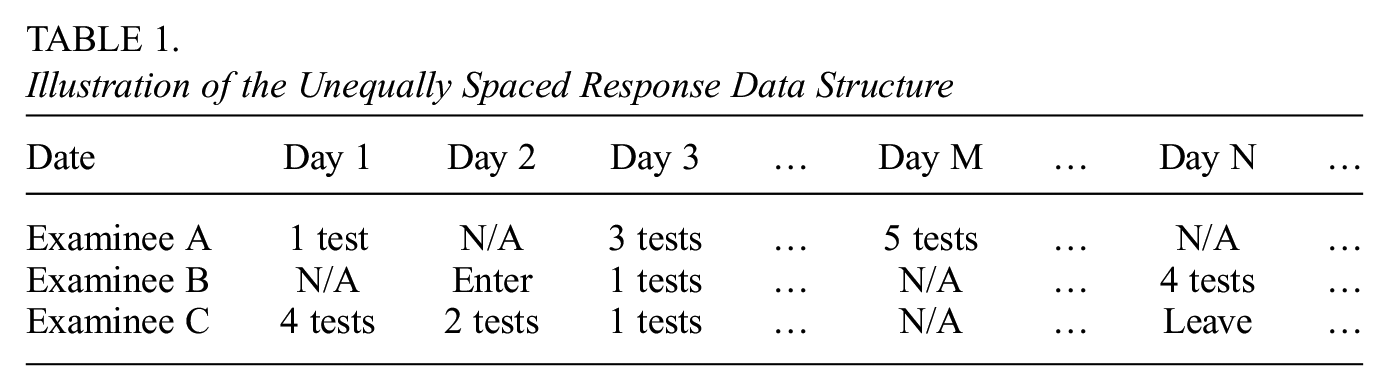
This learning platform continuously yields longitudinal dichotomous observations located at individually varying and irregularly spaced time points, which suggests that we need to model the changes of latent traits using a dynamic structure. Further, according to the test design in EdSphere, there are several existing factors, such as overall comprehension, emotional status, and others (Wang et al., 2013), which would undermine the local independence assumption of classic IRT models. Therefore, we need some new IRT models that can accommodate the modern computerized testing (not merely EdSphere datasets) with the described features above, that is, randomized items, longitudinal observations, and local dependence.
To integrate these features and model the growth of latent traits in computerized testing, Wang et al. (2013) proposed a dynamic IRT model by combining the ideas of parametric functions of time as well as Markov chain models to capture the trajectory of latent traits. They embedded IRT models into a new class of state space models for analyzing longitudinal data located at individually varying and irregularly spaced time points. The trend of the ability growth has been governed by an individually varying parameter,
1.2 Variable Selection With Bayes Factor
Finding variables associated with the “growth factor” in the proposed model is a natural and important question to ask, which can help better understand the features that encourage students’ ability growth. In educational testings, variable selection has been widely considered as it may influence the estimation and predictive accuracy of the model performance (Hamza et al., 2022; Muttakin et al., 2021; Rahman et al., 2017).
For fully Bayesian analysis of variable selection, there are some common techniques often used in literature, such as the deviance information criterion (DIC; Spiegelhalter et al., 2002), the Bayesian lasso (Park & Casella, 2008), the Bayesian spike-and-slab lasso (Ročková & George, 2018), the variational Bayes dynamic variable selection algorithm (Koop & Korobilis, 2018), the Bayes factor (BF) approach (Berger & Pericchi, 1996; Pericchi, 2005) and more recently, the variable selection using reversible jump based on simulating piecewise deterministic Markov processes samplers (Chevallier et al., 2022). Many of these criteria are initially discussed within a linear model framework, and they may be applied to hierarchical models such as the dynamic IRT model under consideration. In this paper, we will use the BF approach for variable selection in our proposed dynamic IRT model. It is not only because BF is a fundamental criterion for model comparison under Bayesian inference, which could be viewed as the Bayesian equivalent of the likelihood ratio test, but also because there is a steady increase in attention to the BF approach as a tool for hypothesis evaluation and model selection in psychological research (Heck et al., 2022; Pan & Yin, 2017; Tijmstra & Bolsinova, 2019).
In addition, the BF has been shown to enjoy good frequentist properties for variable selection in several different types of models. For example, Fernandez et al. (2001) and Liang et al. (2008) discussed some attractive model selection properties for BF under the linear model framework when
However, due to the complex structure of our proposed dynamic IRT model and the high dimensionality of the parameter space, there are no analytical forms available for the BFs of the dynamic IRT models (while noticing there are analytical forms available for the linear regression model discussed in Liang et al., 2008 when
The rest of the paper is organized as follows. In Section 2, we introduce the proposed dynamic IRT model and Bayesian analysis techniques. In Section 3, we propose the method to compute BF with a single MCMC output. Section 4 establishes the model selection consistency for the proposed dynamic IRT model under the mixture of
2. The Proposed Dynamic IRT Model and Bayesian Inference
In this section, we follow the general framework of the dynamic IRT model proposed by Wang et al. (2013) to model the EdSphere dataset but with some changes, where the major change is to introduce an additional level for modeling the “growth factor.” There are several reasons to adopt the general framework of the dynamic IRT model proposed by Wang et al. (2013). The EdSphere dataset is generated from an online learning platform. Thus, the parametric model assumptions we make for the first and second levels come from how the real data was generated from the platform. To be specific, first, the EdSphere test design does not include any item discrimination parameter, and therefore, a one-parameter IRT model is more reasonable in the study of EdSphere datasets. Second, the EdSphere learning platform is in fact a Computer Adaptive Instruction and Testing (CAIT; c.f. Wang et al., 2013 and Swartz et al., 2016, 2011). With CAIT, a test pool of articles is selected for the student based on an estimate of his/her current ability. After the student selects an article from this test pool, the test questions (i.e., items) are then generated before the reading commences according to some prespecified computer protocols. In the current learning platform design, the computational algorithms for the CAIT to estimate his/her current ability are through an autoregressive (AR) model of order 1 to update his/her current ability. Thus, the assumption of an AR(1) model to capture the ability changes would be in alignment with the EdSphere platform design. Hence, based on these two reasons for the EdSphere learning platform design, we specify our proposed model with the one-parameter IRT model in the first level and the AR(1) model in the second level for capturing one’s ability growth, similar to the dynamic IRT models proposed by Wang et al. (2013).
The rest of this section is structured as follows. First, we will introduce our hierarchical model framework, and then discuss the prior choices for unknowns and the corresponding Bayesian computation schemes for our proposed model. Notice that although the discussion of the first and second levels of our proposed model in this section is specifically refers to one-parameter IRT models and AR(1) models, the computational algorithms of BF discussed in Section 3 and the property of the model selection consistency discussed in Section 4 are more general derivations and conclusions for any type of hierarchical models if they can satisfy the mild conditions mentioned in our theorems later. We have provided more details on this point in Section 7.
2.1 Model Settings and Prior Specifications
To analyze dichotomous responses collected at individually varying and irregularly spaced time points, we propose a three-level hierarchical IRT model to capture the changes in ability and associate the changes with certain characteristics of a person. In the first level of our model, the correctness of the items is linked to the latent ability of each individual, the difficulty of the items, and certain random effects. In the second level, it is assumed that the latent ability of the current day depends on the latent ability of the previous day and an increment term related to the time-lapse with uncertainty. These two levels are similar to the dynamic IRT models proposed by Wang et al. (2013). In the third level, we model the relationship of the individual “growth factor”



where
In Level 2,
In Level 3, we use
In the proposed three-level dynamic IRT models, we aim to perform variable selection for the covariates at Level 3, that is, to find all non-zero
Let us define a



Thus, theorems such as model selection consistency proved by Liang et al. (2008) cannot be automatically extended in our model setting since the proper priors has to be used here.
Further, Liang et al. (2008) have pointed out the marginal likelihoods of all models have closed-form expressions when
2.2 Posterior Distribution and Computation
To complete our Bayesian analysis, we further specify the priors for the remaining model parameters as follows: assign (a)
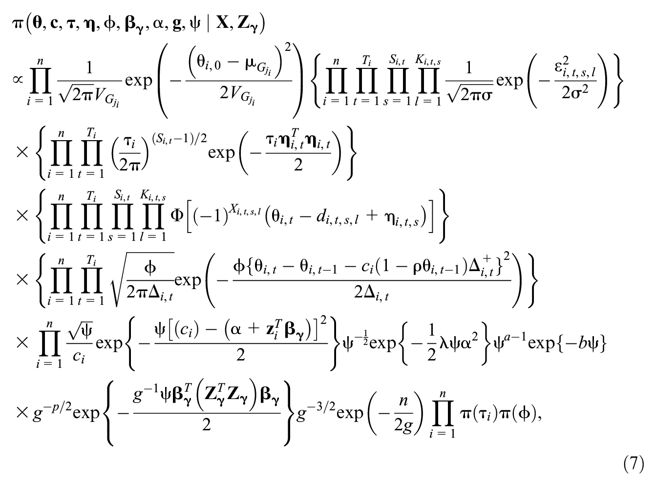
where
Since the joint posterior (7) is not available in the closed form, we develop an MCMC sampling scheme to draw samples from the posterior (7). The sampling procedure of Level 1 and Level 2 are similar to Appendix A of Wang et al. (2013). Thus accordingly, we introduce a latent variable
3. Computing BFs With a Single MCMC Output
In our Bayesian analysis of the proposed IRT models, we can compare different choices of variables in Level 3 using BFs. But to compute BFs, we need to first calculate marginal likelihoods, which usually in practice, are not analytically available. Often, we can numerically calculate them using Monte Carlo methods, such as the Harmonic Mean method (Newton & Raftery, 1994), the Chib method (Chib, 1995), the Stepping Stone method (Xie et al., 2011), just naming a few. Recently, Y. Liu et al. (2019) have given a thorough comparison of the most commonly used Monte Carlo methods for computing the marginal likelihood of IRT models.
However, due to the complex structure and high dimensionality of the parameter space in the proposed dynamic IRT model, computing the marginal likelihood for each corresponding model in the variable selection with existing Monte Carlo methods is very challenging. In the paper of Verdinelli and Wasserman (1995), they presented the generalized version of Savage–Dickey (SD) density ratio to compute BF by multiplying a correction term with the SD density from Dickey and Lientz (1970). In M.-H. Chen (2005), they further developed an approach to obtain the BF of each model versus the full model using only a single MCMC output yielding from the full model based on the extension of the generalized SD ratio from Verdinelli and Wasserman (1995).
Motivated by the idea from M.-H. Chen (2005) to compute BF efficiently in a single MCMC output, we formally define notations of the models under comparison as follows. Let
We will use priors specified in Section 2 for all unknown parameters and apply a uniform prior on the model space following Liang et al. (2008). Based on the current linear structure at Level 3, we have the identity

holds, which leads to the proposition below.

and the BF of the null model

where both expectations (9) and (10) are taken w.r.t.
We use the

Notice that Equations (9) and (11) in Proposition 1 are in a similar structure as what was presented in Theorem 2 of M.-H. Chen (2005), but we have shown that it is applicable in the hierarchical model framework. Further, unlike the generalized version of the SD density ratio in Verdinelli and Wasserman (1995), both expectations (9) and (10) are taken w.r.t. the posterior of
Next, using the assigned prior distribution for
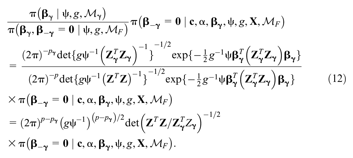
Here,

with

Similarly, we can derive,

Then, after some math simplification, we can write out the quantity inside the expectation of Equation (10) as the expression below:
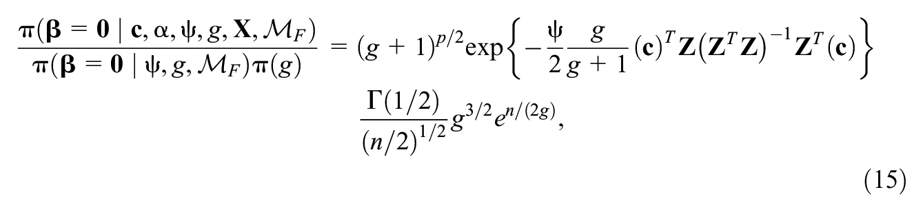
by noticing that
4. Model Selection Consistency
A major motivation to use the BF as the variable selection tool is its attractive model selection properties discussed in Liang et al. (2008). In Liang et al. (2008), they pointed out under the linear model setup,

Further, in Theorem 3 of Liang et al. (2008), they showed that when the Zellner–Siow prior is used and for any model

where

In the proposed dynamic IRT model, modeling
However, the proof for the model selection consistency in Liang et al. (2008) could not be directly applied here. To note, we could not employ the non-informative priors assigned in Liang et al. (2008) for the precision parameter
4.1 Model Consistency of the Proposed Dynamic IRT Model
Let us first focus on the general linear model used by Liang et al. (2008) and add the superscript in

where
Without loss of generality, we assume the columns of
Now, using Lemma 1, we can further prove the model selection consistency of the dynamic IRT model. The following Theorem 2 states the model selection consistency of the dynamic IRT model, and we provide the details of the proof in Supplemental Appendix D (available in the online version of this article).
Further, follow the definition of

for all
5. Simulation Study
Though the proposed BF approach is supported by Theorem 2 for the posterior model selection consistency, it is desirable to examine the performance of this approach in finite samples. Thus, we design and carry out several simulations in this section.
Let us consider four choices for the number of sample size of individuals, that is,
In addition, the first five covariates
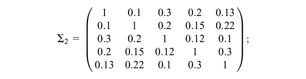
while the last five covariates
Using the data generation scheme described above, we carry out the simulations with 100 different random seeds for each case of coefficients
5.1 Case 1:
In this simulation study, from Table 2, we see that the percentage of using BF approach to select the right model among 100 simulations is steadily increasing when the sample size increases for all three settings of
Percentage of the True Model Ranked as the “Best” Model by the Bayes Factor Approach Among 100 Simulations

For
Quantities for Assessing Estimation of

Note. CP = coverage probability; RMSE = root mean square error.
5.2 Case 2:
In this simulation study, we assume the full model be the true model. Similar to the output in Case 1, from Table 4, we have seen that when
Percentage of the True Model Ranked as the “Best” Model by the Bayes Factor Approach Among 100 Simulations

Quantities for Assessing Estimation of
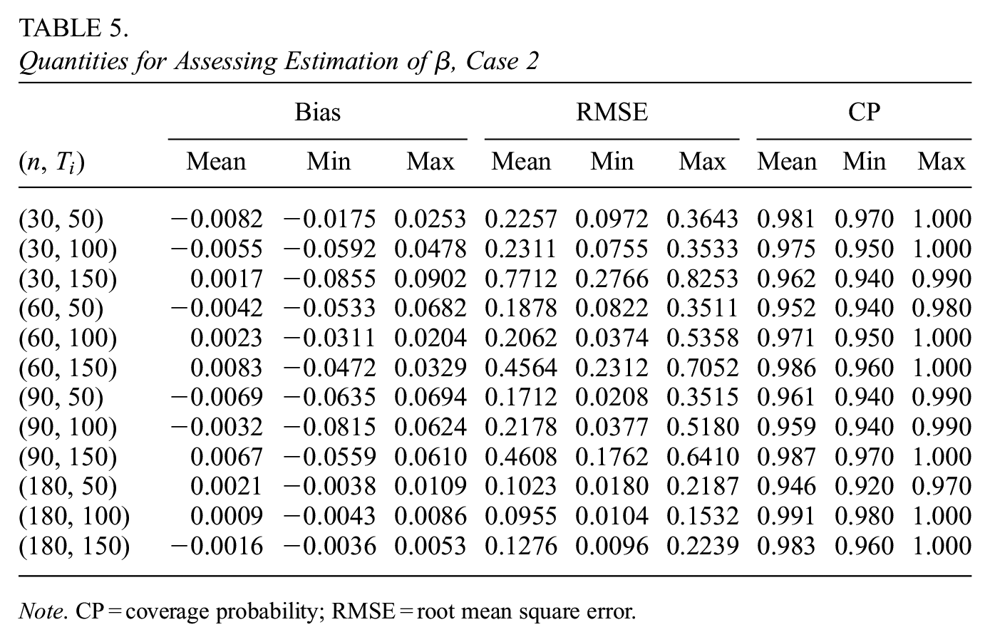
Note. CP = coverage probability; RMSE = root mean square error.
5.3 Case 3:
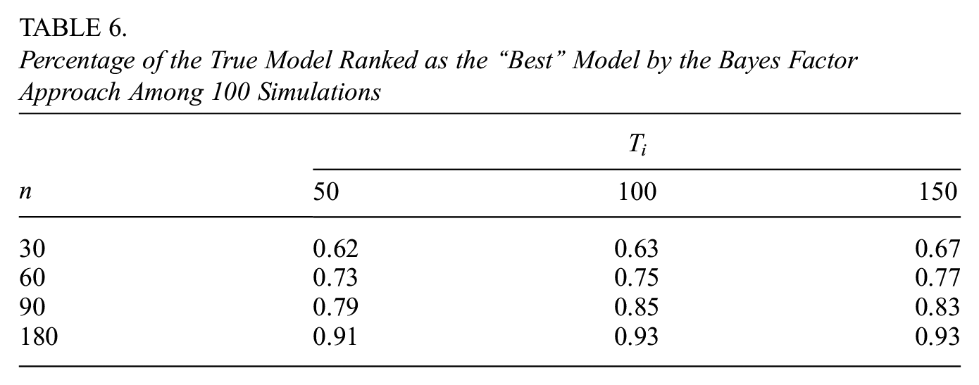
In this simulation, we consider a case when there are a fewer number of non-zero coefficients. In Table 6, we have also seen that there is an increasing trend for the probability of selecting the true models, which conforms to the theoretical trend indicated in Section 4. In Table 7, we have represented all quantities related to how well the estimation of
Percentage of the True Model Ranked as the “Best” Model by the Bayes Factor Approach Among 100 Simulations
Quantities for Assessing Estimation of

Note. CP = coverage probability; RMSE = root mean square error.
6. Real Data Application
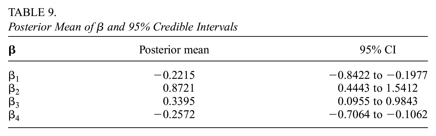
The simulation study in Section 5 shows the finite sample performance of our proposed method is consistent with the theoretical results we derive. Thus, we are confident to apply the proposed method to the EdSphere dataset. In this analysis, 54 students are randomly selected in the data, and 4 candidate covariates are used: gender, economic status, race, and preLexile score, where we denote them by
Then, we run the MCMC procedure with 120,000 iterations for the joint posterior of the unknown parameters in the full model and discard the first 20,000 MCMC samples as a burn-in period. Then, we employ the proposed BF approach in Section 3 to compute the BFs for different combinations of covariates used in Equation 3, and then the results of the BF are summarized in Table 8. A total of 120,000 iterations of the MCMC algorithm will take about 12 hr for a Core i5—8GB RAM laptop but the comparison between BFs only takes less than 2 min. Generally speaking, the computation speed for the model comparison part is very fast. We have employed the Geweke Convergence test (Geweke, 1992) and the Heidelberger & Welch stationary test (Heidelberger & Welch, 1983) to test the convergence of MCMC chains for all parameters and we have used the R package
Estimated the Logarithm of BF (
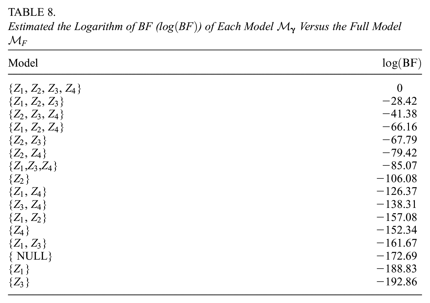
From Table 8, we see that the model with the largest BF comparing to the full model is the full model itself, that is, including the gender, race, economic status and preLexile in terms of explaining the growth factor
Posterior Mean of
7. Discussion
From the simulation results, we can see that the BF approach seems to be a reliable tool for variable selection in the proposed dynamic IRT model, especially when the sample size is relatively moderate to large. In general, computing the marginal likelihoods of hierarchical models with multi-levels is difficult if no analytical forms are available, and the usage of the BF may be limited. However, if one wants to perform the variable selection under a hierarchical model, at a single, “stand-alone” layer that consists of the linear structure similar to Level 3 as in our proposed hierarchical model, Proposition 1 may still be applied in a similar fashion to compute the BFs conveniently. The proof for posterior model selection consistency may also hold if (a) similar assumptions as those stated in Theorem 2 hold and (b) the layer we consider to do variable selections links with other layers in certain ways, for example, the parameters in the considered layer are not included in any other layers.
There are also other model selection criteria for hierarchical models, such as the widely applicable information criterion (WAIC; Watanabe, 2010) and DIC (Spiegelhalter et al., 2002) in the literature. When applying the DIC for model selection, often the “focus” of the parameters of interest may affect the results. One may integrate out all “intermediate” parameters to obtain the likelihood with respect to the parameters of interest, which is usually challenging in hierarchical models such as the complex IRT models discussed in the paper, or one may treat the likelihood conditioning on the “intermediate” parameters. But the latter way has several criticisms (F. Liu et al., 2022 and the reference therein). In our future work, it would be great interesting to compare the model selection performances of these criteria in comparison to the BF approach we used here.
The current variable selection algorithm requires comparisons of BFs for all possible submodels. Under a low-dimensional setting of predictors, the time taken to explore the model space is not a issue. For large amount of predictors, to go through the whole model space within a finite time interval might be impossible. Thus, how to explore the model space in order to find the best model using BFs will be an interesting topic to study.
Supplemental Material
sj-pdf-1-jeb-10.3102_10769986251314527 – Supplemental material for Bayesian Variable Selection in Dynamic Item Response Theory Models
Supplemental material, sj-pdf-1-jeb-10.3102_10769986251314527 for Bayesian Variable Selection in Dynamic Item Response Theory Models by Jingyu Sun, Yang Liu, Xiaojing Wang and Ming-Hui Chen in Journal of Educational and Behavioral Statistics
Footnotes
Declaration of Conflicting Interests
The author(s) declared no potential conflicts of interest with respect to the research, authorship, and/or publication of this article.
Funding
The author(s) disclosed receipt of the following financial support for the research, authorship, and/or publication of this article: The research of Dr. J. Sun and Dr. X. Wang was supported by the National Science Foundation under Grant No. 1848451.

Authors
References
Supplementary Material
Please find the following supplemental material available below.
For Open Access articles published under a Creative Commons License, all supplemental material carries the same license as the article it is associated with.
For non-Open Access articles published, all supplemental material carries a non-exclusive license, and permission requests for re-use of supplemental material or any part of supplemental material shall be sent directly to the copyright owner as specified in the copyright notice associated with the article.
