
Abstract
Accurate estimation of latent traits is critical in educational and psychological measurement, yet establishing validity evidence is challenging under small samples, ordinal data, and skewed distributions. We propose a Bayesian framework that incorporates expert-informed priors to enhance estimation and validity evidence for multi-unidimensional instruments. Simulation studies demonstrate that expert input improves estimation accuracy over ordinal confirmatory factor analysis, especially in samples as small as N = 25, with diminishing returns beyond six to nine experts. We compare variational inference (automatic differentiation variational inference) and Hamiltonian Monte Carlo in terms of estimation accuracy, computational efficiency, and posterior quality. A real-world application using TIMSS Grade 8 Mathematics data illustrates practical implications for expert selection and estimation strategies in small-sample instrument development.
Keywords
Introduction
Educational and psychological tests are essential for measuring individuals’ latent abilities or traits, which are unobservable but inferred through carefully designed instruments. These tests are widely used in state-level assessments (e.g., Massachusetts Comprehensive Assessment System [MCAS]), national assessments (e.g., National Assessment of Educational Progress [NAEP]), and international assessments (e.g., Trends in International Mathematics and Sciences Study [TIMSS]). The results provide policymakers and educators with critical information about student achievement and areas needing improvement. Similarly, tools like the Classroom Assessment Scoring System Toddler (Pianta et al., 2008) help educators evaluate classroom interactions to enhance teaching quality and student learning.
Multi-unidimensional instruments play a vital role in measuring complex constructs such as critical thinking or depression by assessing multiple distinct but related traits through subtests (e.g., TIMSS mathematics assessment; Lindquist et al., 2017). Test development is a rigorous, multi-stage process requiring validity and reliability evidence at the instrument and item levels (Crocker & Algina, 1986; DeVellis, 1991). Content validity is often established through expert reviews, while construct validity relies on factor analysis using participant data. However, traditional methods analyze these components separately, requiring large samples and prolonged timelines, often spanning years (Ellis et al., 2009).
Small sample sizes present significant challenges to instrument development. In niche populations, such as individuals with rare conditions, ethical or logistical constraints may limit participation (Burns & Grove, 2010; Patel et al., 2003). Smaller samples result in unreliable parameter estimates, inflated measurement error, and model convergence issues (Linacre, 1994; Stone & Yumoto, 2004). Additionally, the ordinal nature of response data, common in educational and psychological research (e.g., Likert scales), complicates validity testing. Maximum Likelihood estimation, the standard approach in confirmatory factor analysis (CFA), assumes continuous, normally distributed data and struggles with ordinal scales, often yielding biased parameter estimates and unreliable fit indices (Brown, 2006; Flora & Curran, 2004).
To address these challenges, Bayesian methods have emerged as a promising alternative. Gajewski et al. (2013) proposed a Bayesian framework integrating content and construct validity using expert ratings as priors to reduce sample size requirements. Building on this, Jiang et al. (2014) introduced the Bayesian Instrument Development (BID) method, incorporating Fisher’s transformation to allow full-range correlations, achieving better precision and efficiency compared to traditional CFA. Garrard et al. (2015) extended these methods to ordinal data with their Ordinal BID approach, enhancing predictive validity and parameter estimation for small samples.
Despite these advancements, prior studies are limited to unidimensional models and fail to address multidimensional instruments commonly used in educational and psychological assessments (Sheng & Wikle, 2007). To overcome these gaps, our study introduces a novel Bayesian framework for developing multi-unidimensional instruments, integrating expert and participant data, and leveraging state-of-the-art tools like Stan (Stan Development Team, 2023). Stan’s Hamiltonian Monte Carlo (HMC) algorithm offers improved sampling efficiency and enables advanced model evaluation techniques. To further enhance computational efficiency, we incorporate Variational Approximation, which transforms Bayesian inference into an optimization problem (Kucukelbir et al., 2017).
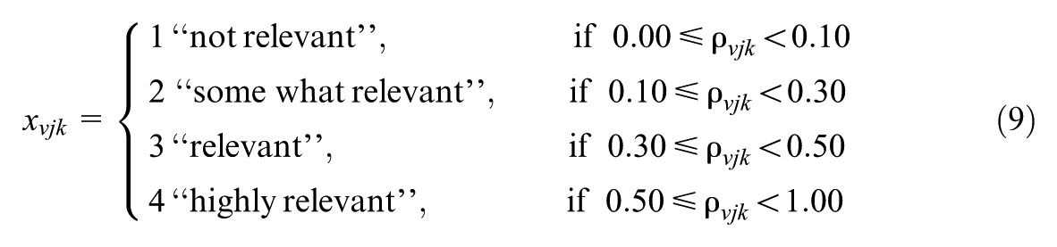
Purpose and Research Questions
The main purpose of this study is to develop a Bayesian framework that integrates expert opinions and participant data to establish validity evidence for multi-unidimensional instruments. Through extensive simulations, this study evaluates parameter estimation accuracy and computational efficiency under small-sample conditions. The specific research questions are as follows:
The organization of this paper is as follows. The next section presents Methodology, which introduces item response theory (IRT), multi-unidimensional IRT models, the hierarchical Bayesian framework, and parameter estimation techniques (HMC, automatic differentiation variational inference [ADVI]), followed by our proposed Bayesian modeling framework to establish validity evidence for multi-unidimensional instruments, including model formulation, prior specification, and parameter estimation. Section “Simulation Studies” illustrates the simulation designs addressing our research questions. Section “Results” presents findings from the two simulation studies. Section “Empirical Study” applies the framework to TIMSS 2019 Grade 8 Mathematics Student Questionnaire data. Sections “Discussion and Conclusion” and “Limitation and Future Research” summarize key findings, implications, limitations, and future research directions.
Methodology
IRT and Multi-Unidimensional IRT Models
IRT, also known as latent trait theory, is a modern framework for evaluating assessments by modeling the relationship between item responses and underlying latent abilities using person and item parameters. Developed by scholars such as Lord, Rasch, and Novick in the 1950s and 1960s, IRT yields robust, sample-independent estimates that overcome many limitations of Classical Test Theory, making it widely applicable in educational, psychological, and health-related assessments (van der Linden & Hambleton, 2013). Multidimensional IRT (MIRT) extends this framework to accommodate multiple latent traits or uncertain test structures (Reckase, 1997, 2006), while multi-unidimensional instruments—comprising subtests that each measure a specific ability yet capture inter-dimensional correlations—are particularly valuable for designing, maintaining, and equating assessments such as personality tests and achievement batteries (Sheng & Wikle, 2007).
In a multi-unidimensional test comprising

where
In Equation 1, Φ(⋅) is the standard normal cumulative distribution function, as the link makes this a normal-ogive or probit IRT model, which is a common formulation in multidimensional IRT. If instead the logistic function
Both ability
Standardizing
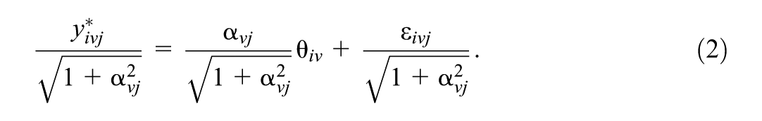
This connects to a factor analysis model:

where
A Hierarchical Framework for Bayesian Item Response Modeling
Bayesian IRT emerged in the 1980s to address challenges of complex response behaviors and hierarchical data structures (Fox, 2010). Researchers like Swaminathan and Gifford (1982, 1985), Rigdon and Tsutakawa (1983), and Mislevy (1986), among others, pioneered Bayesian methods to model guessing, extreme responding, missing data, and intentional misrepresentation. A key strength of the Bayesian approach lies in its ability to incorporate prior knowledge to improve the accuracy of parameter estimates when sample sizes are small. Furthermore, this approach provides a flexible framework for analyzing survey data with intricate hierarchical structure (Fox, 2010).
The hierarchical framework for item response modeling consists of two levels to account for the relationship between the item and person parameters.
At the first level, an item response model captures the probabilities of individual responses. Let

The second level describes population-level characteristics for both items (in Equation 6) and examinees (in Equation 7), with each parameter being assigned a prior distribution and a joint distribution at the population level:


With the two-level models described above, the full joint posterior distribution of

Bayesian Parameter Estimation Techniques
Advances in computational statistics have revolutionized parameter estimation in IRT models, particularly through the development of sampling-based techniques like Markov Chain Monte Carlo (MCMC) and variational inference techniques. Among MCMC methods, HMC has gained prominence for its efficiency in sampling from complex, high-dimensional posterior by leveraging Hamiltonian dynamics (Duane et al., 1987; Neal, 2011). HMC introduces auxiliary momentum variables, uses the leapfrog integrator to simulate motion through an energy landscape, and employs a Metropolis acceptance criterion to ensure convergence (see Appendix A).
In contrast, ADVI approximates posteriors by transforming them into a standard coordinate space and fitting a simple variational distribution—typically a diagonal Gaussian—via optimization of the evidence lower bound (ELBO; Kucukelbir et al., 2017). While ADVI offers significant computational efficiency for large-scale or high-dimensional models, its mean-field assumption may limit its capacity to capture parameter dependencies (see Appendix B).
Bayesian Multi-Unidimensional IRT Models
Consider a
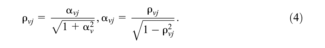
Prior Specification From Expert Ratings
Following Gajewski et al. (2011), experts’ ratings on an item’s relevance are used to inform priors for the item’s correlation parameter
Similarly, ratings for between-dimension correlations (
where
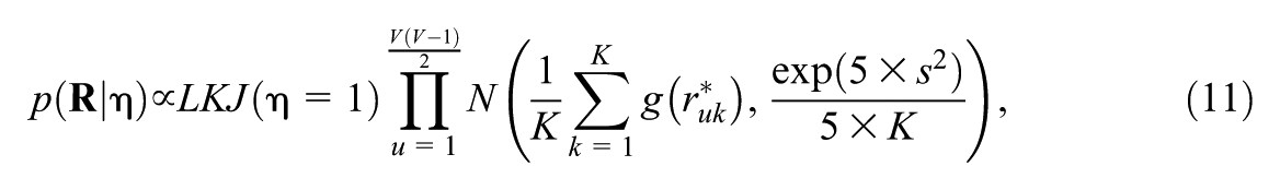
where
The LKJ prior is widely applied in Bayesian hierarchical and multivariate modeling because it places a proper distribution on valid correlation matrices (symmetric, positive-definite, ones on the diagonal) and is controlled by a shape parameter η. When η = 1, the prior is uniform over all correlation matrices, avoiding any preference for particular structures. We adopted this noninformative setting so that the data and expert-informed priors, rather than strong distributional assumptions, determine the estimated correlations.
Transition parameters
The full posterior distribution is given by

Simulation Studies
Simulating Experts’ Rating
Following Jiang et al. (2014), we assume experts unanimously interpret correlations in relation to item relevance and that their ratings align with participants’ response patterns. To simulate item-to-dimension correlations, we adopt Garrard et al.’s (2015) approach by incorporating low (.3), moderate (.5), and high (.7) correlations, with all simulations conducted using R 4.1.2 (R Core Team, 2022).
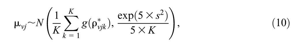
Experts’ ratings are simulated using the Rating Scale Many-Facet Rasch (RS-MFR) model (Andrich, 1978; Linacre, 1989). Specifically, the log-odds of expert
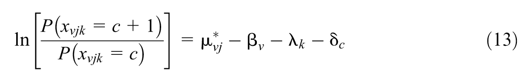
where
Simulation Study One
The first simulation study is designed to address Research Question 1 by comparing Bayesian methods using expert-informed priors with ordinal CFA and determining the number of experts needed to match the accuracy of a doubled sample size. A six-way factorial design is used with factors: number of dimensions (
Participants’ abilities
Standardized responses are generated using
For each item, convert
Generate 100 replications for each of the 864 scenarios.
Parameter Estimation
CFA baseline: The ordinal CFA model is estimated using WLSMV estimator provided by the “lavaan” R package (Rosseel, 2012). WLSMV (Weighted Least Squares Mean and Variance adjusted; Muthén et al., 1997) is widely used in structural equation modeling for categorical indicators (binary or ordinal). It operates on polychoric or polyserial correlations, minimizes the weighted difference between observed and model-implied statistics, and adjusts chi-square tests and standard errors for non-normality and non-continuity.
Bayesian IRT model: Experts’ ratings are simulated using the rating scale model (Equation 13), with varying numbers of experts
Model Performance Comparison
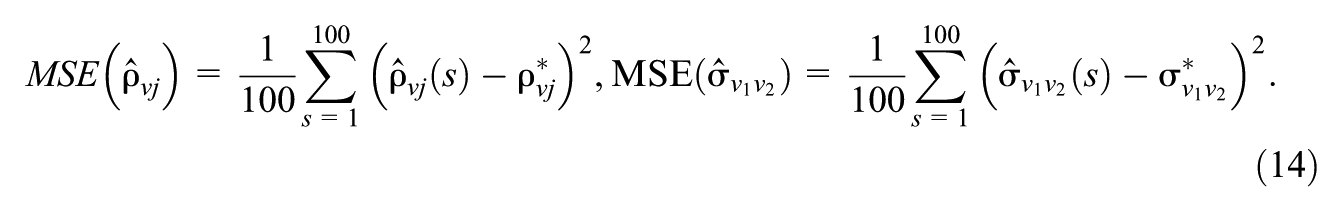
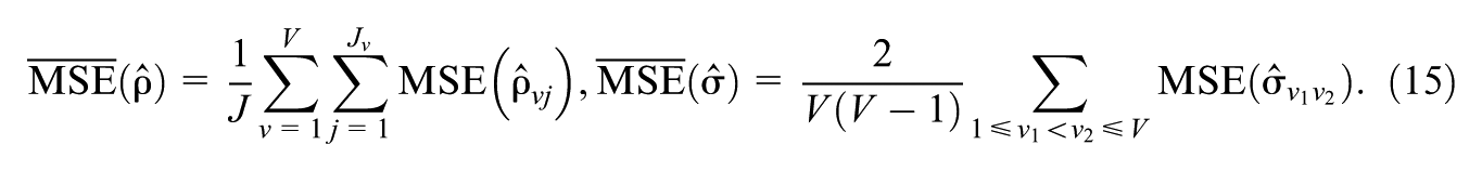
The average mean squared error (MSE) is used as the metric to compare estimation accuracy across models and different numbers of experts. Lower values indicate greater accuracy.
Let
The MSE for each
The average MSEs for
Mixing Quality of HMC Sampling
The mixing quality of HMC sampling is assessed using Gelman’s
Comparison of Sample Size
with
Experts Versus
Using Non-Informative Priors
This analysis refers to a prior sensitivity analysis to assess the value of expert-derived priors in enhancing estimation accuracy. Specifically, we determine the number of experts
Simulation Study Two
The second simulation study is designed to answer Research Question 2—how variational approximation (ADVI) compares to HMC in terms of estimation accuracy, computational efficiency, and approximation quality under various conditions? Simulated datasets are again generated using the same data simulation method described in Simulation Study One, following the same six-way factorial design, except for response category C = 4, and response distribution
Parameter Estimation
Experts’ ratings are again simulated using the rating scale model (Equation 13), with the number of experts set based on findings from Simulation Study 1. Priors are then specified according to the simulated ratings following Equations 10 and 11.
ADVI and HMC are employed in parallel to estimate the model parameters:
HMC: Sampling from the full posterior using the HMC algorithm with the NUTS, implemented via the CmdStanR package (version 0.7.0) in R 4.1.2. The sampling procedure consists of 4,000 iterations, with a 2,000-burn-in period, across four chains.
ADVI: Approximating the full posterior using ADVI with a mean-field Gaussian variational family. The ADVI process was run for a maximum of 3,000 iterations, with 50 Monte Carlo Samples for estimating ELBO gradients and 100 Monte Carlo Samples for the ELBO estimate. Implementation was also done using the CmdStanR package (version 0.7.0) in R 4.1.2.
Model Performance Comparison
Estimation Accuracy: We compare HMC and ADVI using the average MSEs of
Computational Efficiency: For each scenario, we compare the average runtime of HMC with the NUTS and ADVI to determine which method is more efficient.
Approximation Quality of ADVI: To check the approximation quality of ADVI, we compare ADVI’s results to those from HMC, which is considered the gold standard in Bayesian inference. Specifically, we use the Kolmogorov–Smirnov (KS) test (Kolmogorov, 1933; Smirnov, 1948) to compare ADVI’s posterior estimates with HMC’s samples. We then measure ADVI’s overall performance by calculating the fraction of parameters for which the KS test p-value is greater than .05, indicating a good approximation.
Results
Results for RQ1: Expert-Informed Priors Improve Estimation Accuracy
This section presents two analyses: (a) Parameter estimation accuracy comparisons between the Bayesian method and ordinal CFA, with an assessment of mixing quality for HMC sampling. (b) Comparison of a sample size
Parameter Estimation Accuracy: Bayesian Method Versus Ordinal CFA
Figures 1 and 2 compare the average MSEs for
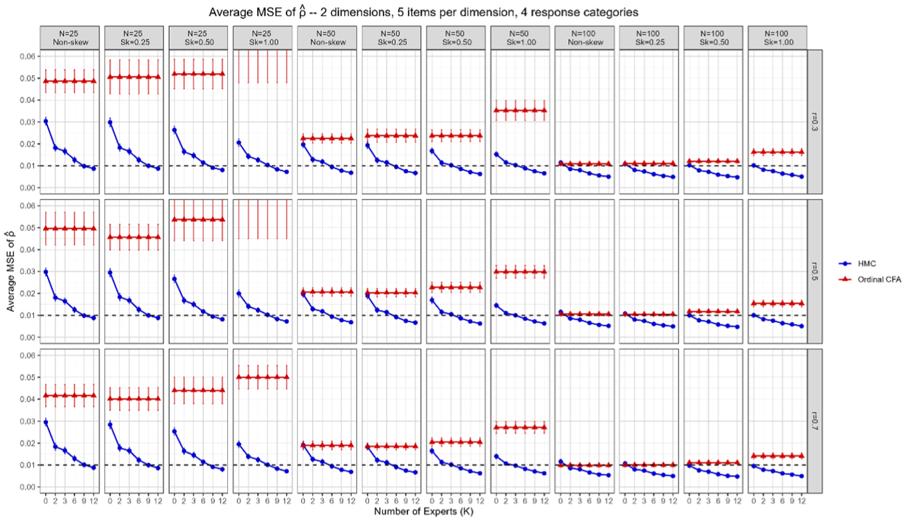
Comparisons of average MSEs of
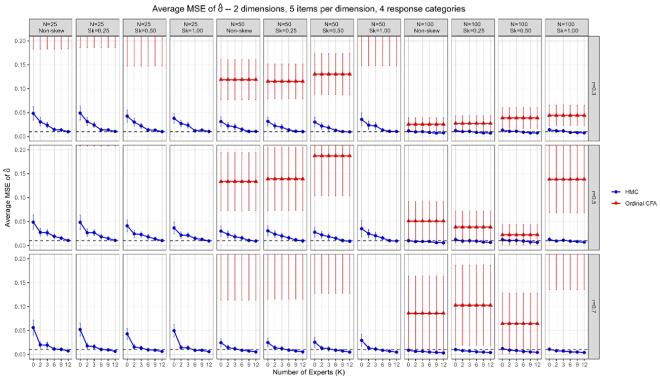
Comparisons of average MSEs of
The Bayesian method, using priors from at least six experts, consistently yields lower MSEs for
Estimation accuracy declines with increasing dimensions for both methods, but ordinal CFA is more adversely affected—especially in small samples—while the Bayesian method remains stable. Ordinal CFA benefits from more items per dimension, whereas the Bayesian method’s performance is unaffected by item count. Additionally, increasing the number of experts markedly improves the Bayesian method up to six experts, with further increases offering diminishing yet positive returns.
The Bayesian method also consistently outperforms ordinal CFA in estimating between-dimension correlations
Figures 1 and 2 reveal two divergent patterns between CFA and Bayesian estimation. First, CFA’s estimation of item-to-dimension correlations (ρ) improves as the between-dimension correlation (r) increases from .3 to .7. Stronger correlations across subtests increase shared variance, which stabilizes the factor loading estimates that underlie ρ. Second, the opposite occurs for CFA’s estimation of between-dimension correlations (σ): higher r values reduce the effective variability among dimensions, making σ more difficult to estimate accurately, especially in small samples. By contrast, the Bayesian approach with HMC exhibits relative stability in estimating both ρ and σ, as the posterior distribution incorporates prior information and fully accounts for uncertainty.
Mixing Quality of HMC Sampling Versus Convergence of Ordinary CFA
The purpose of assessing HMC sampling quality was to verify that including experts improved not only estimation accuracy but also convergence. We evaluated mixing quality using the
In contrast to zero non-convergence in HMC, CFA exhibited some notable convergence issues (Table S2). Across 864 scenarios varying in sample size (N = 25, 50, 100), factor correlation (r = .3, .5, .7), and response distribution (non-skewed vs. skewed, sk = 0.25, 0.5, 1), non-convergence was concentrated in small samples (N = 25), particularly under severe skewness (up to 28% at r = .3, 26% at r = .5, and 22% at r = .7). By N = 100, convergence failures were nearly eliminated (<0.3%). Although higher r slightly reduced failure rates, skewness effects remained substantial at N = 25. These results indicate that CFA is prone to instability in small, skewed samples but stabilizes rapidly with moderate sample sizes (N ≥ 50).
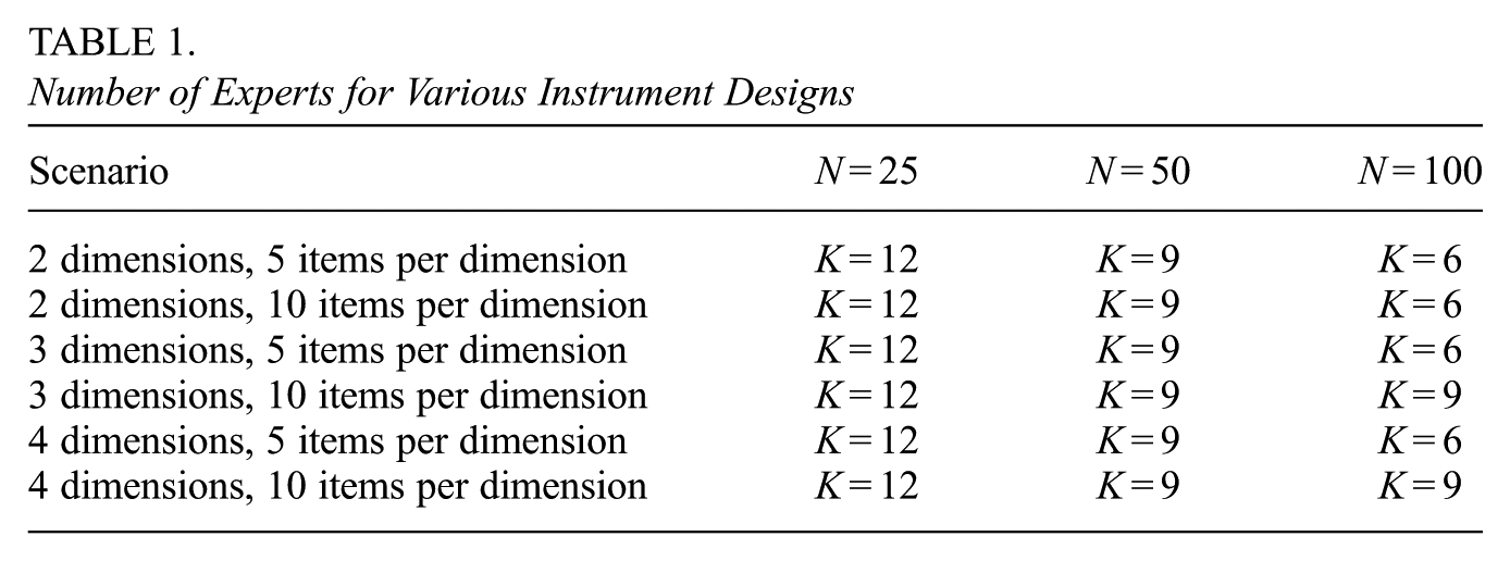
Table 1 summarizes the recommended number of experts ensuring estimation accuracy for both
Number of Experts for Various Instrument Designs
Comparisons of Sample Size
with
Experts Versus
Using Non-Informative Priors
The average MSEs of
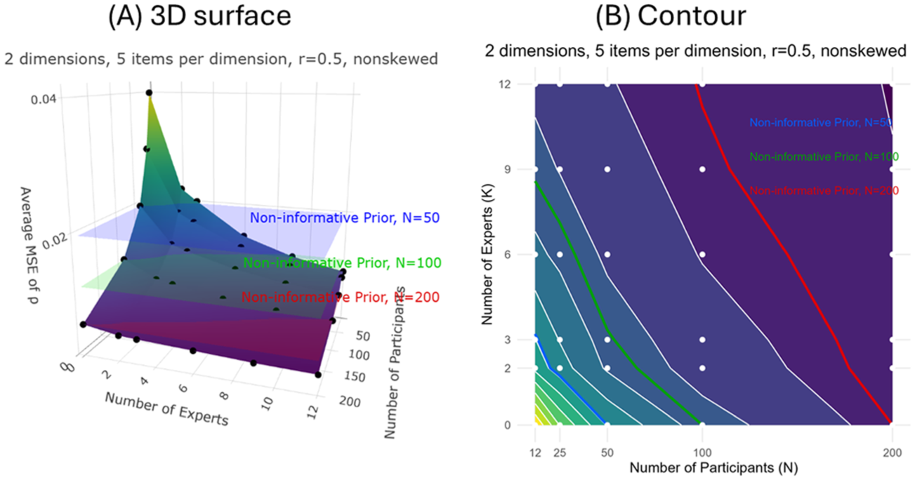
Comparisons of average MSEs of
Reciprocal MSE Modeling: Contributions of Factors
Estimation accuracy, measured by MSE, is known to be inversely proportional to sample size (MSE ∝ 1/N, or equivalently 1/MSE ∝ N). Rather than modeling MSE directly, which produces a nonlinear relationship as shown in Figure 3, we examined its reciprocal (1/MSE), which reveals a simple and additive linear relationship with number of experts (K) and sample size (N), as illustrated in Figure 4.
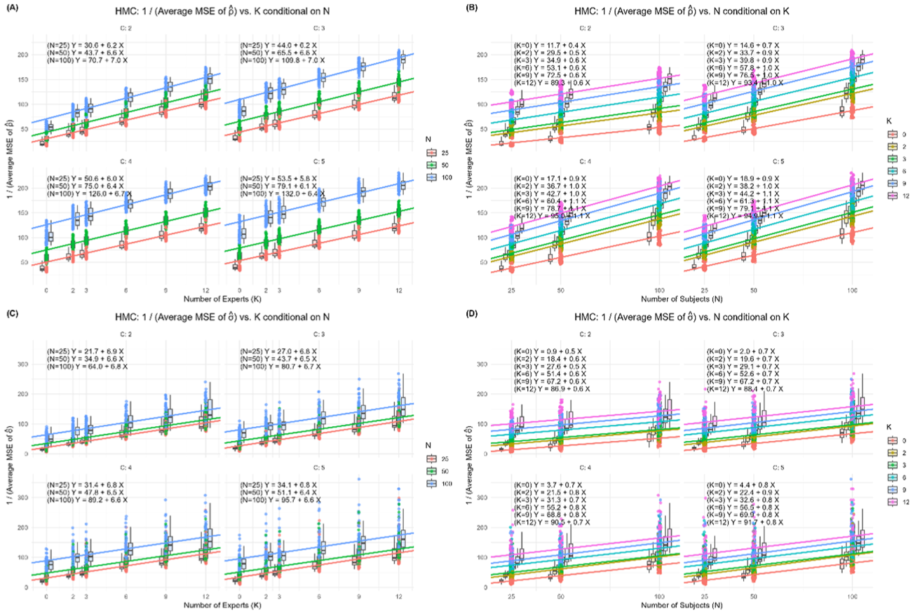
Estimation accuracy of item–trait correlations
To further investigate the relative importance of the simulation factors, we conducted a forward selection regression analysis using 1/MSE of
Forward Selection Results on Estimation Accuracy of
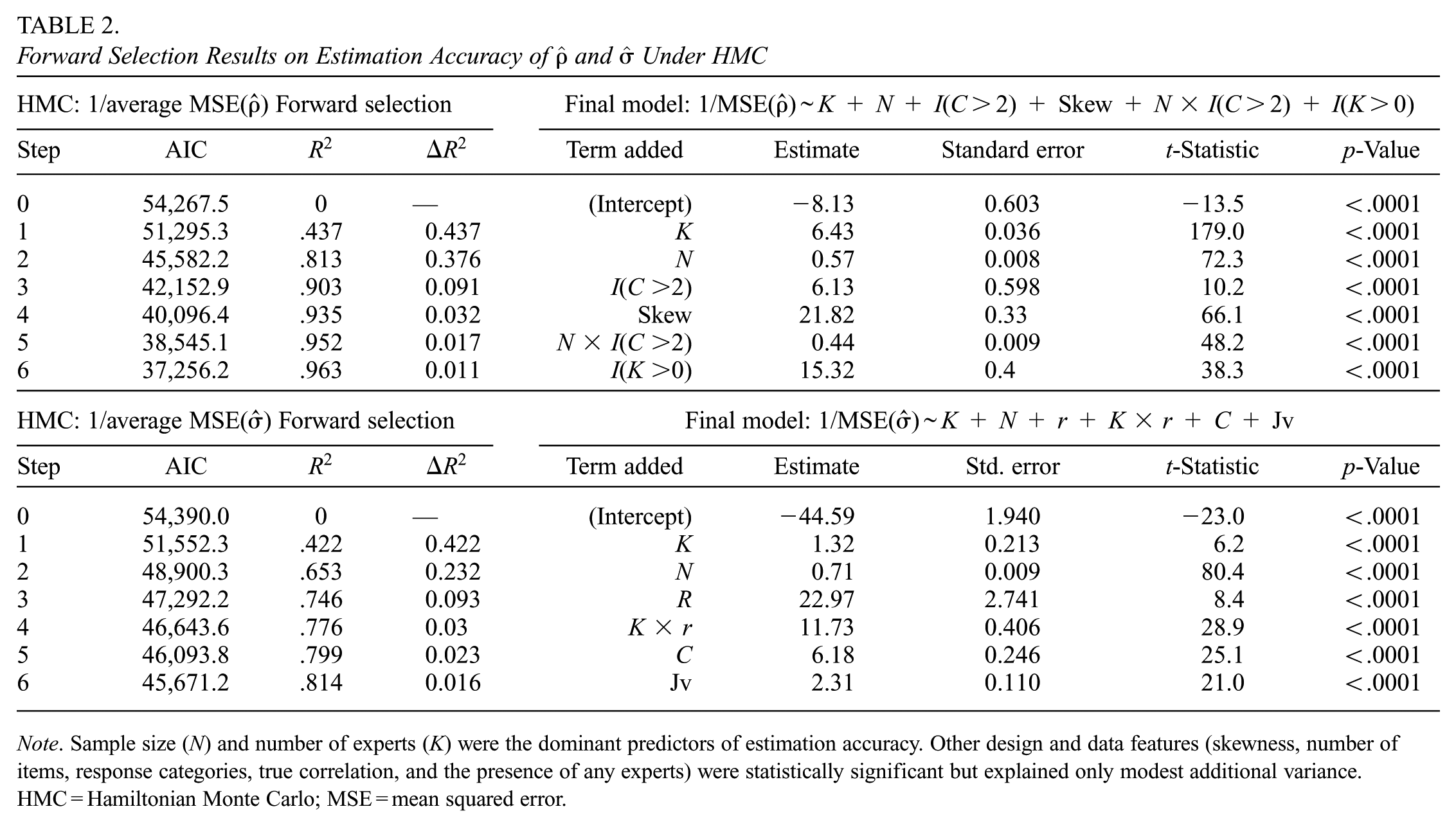
Note. Sample size (N) and number of experts (K) were the dominant predictors of estimation accuracy. Other design and data features (skewness, number of items, response categories, true correlation, and the presence of any experts) were statistically significant but explained only modest additional variance. HMC = Hamiltonian Monte Carlo; MSE = mean squared error.
The forward selection results show that sample size (
Based on the relative ratios of the coefficients, we derive equivalences between the number of experts and sample size: for item–trait correlations
In addition to the dominant roles of sample size (N) and number of experts (K), several other factors made statistically significant, though comparatively modest, contributions to estimation accuracy (Table 2). For
The full model equations in Table 2 can be used to guide study design. For example, if a precision criterion is set such that MSE(
Results for RQ2: HMC Versus ADVI Comparison
Parameter Estimation Accuracy: ADVI Versus HMC
Figures 5 and 6 present the comparisons of average MSEs and squared bias of
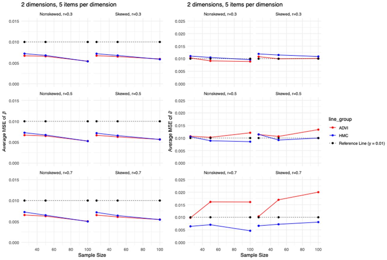
Comparisons of average MSEs of
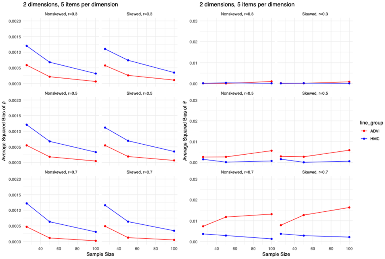
Comparisons of average squared bias of
Overall, the results show the complementary strengths of ADVI and HMC. ADVI consistently demonstrated superior performance in estimating
Preferred Estimation Methods by Instrument Design and Sample Size
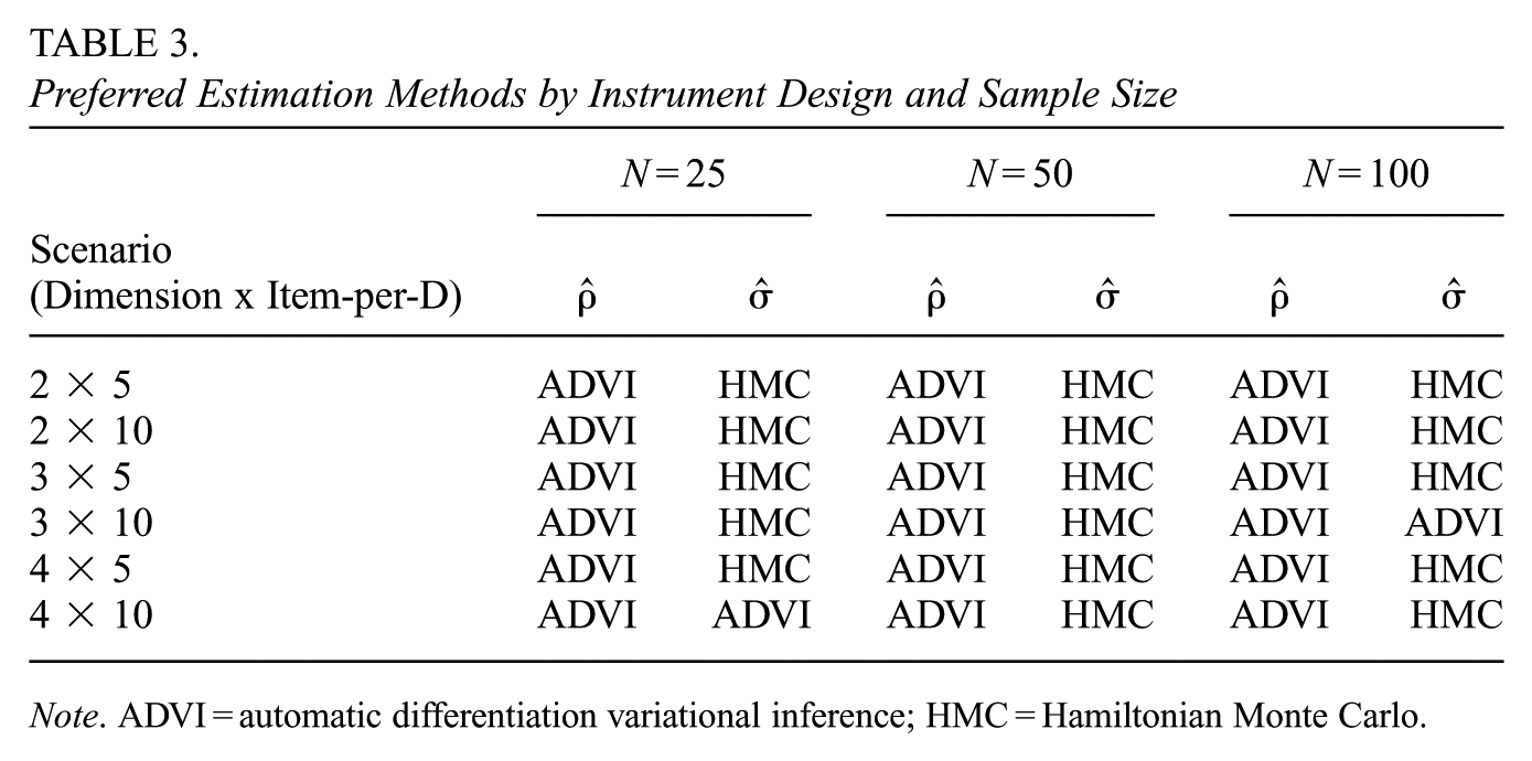
Note. ADVI = automatic differentiation variational inference; HMC = Hamiltonian Monte Carlo.
Computational Efficiency: ADVI Versus HMC
For each simulation using HMC, the average runtime for 4,000 iterations (2,000 burn-in and 2,000 sampling) across four chains was recorded. ADVI used an adaptive stopping criterion, terminating optimization when the relative change in ELBO fell below 0.01 (up to 3,000 iterations), using 50 samples for gradient estimation and 100 for ELBO calculation.
Figure 7 (with additional comparisons in Figures S26–S30 in the Supplemental Material in the online version of the journal) shows that while runtimes for both methods increase linearly with sample size, HMC consistently took longer runtimes than ADVI, with the gap widening significantly as sample size, number of dimensions, or the number of items per dimension increased. For example, at
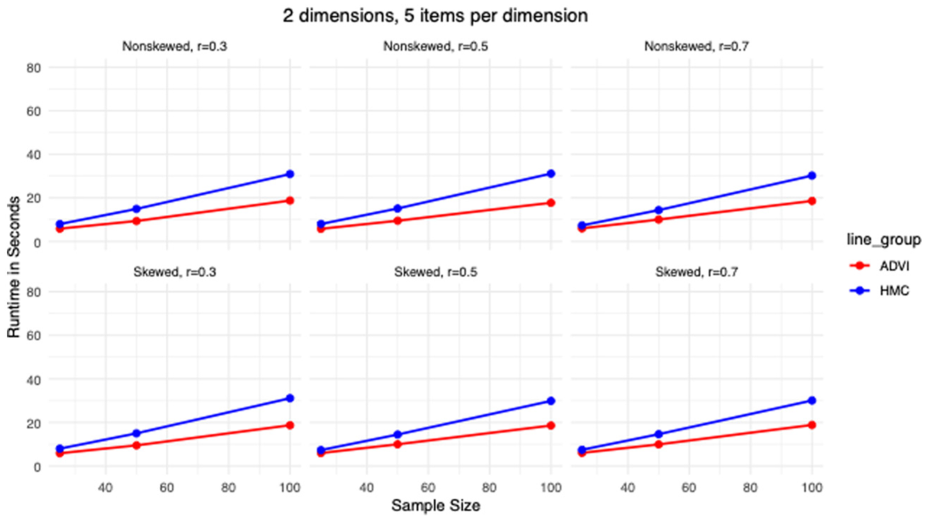
Comparisons of average runtime of HMC and ADVI for a 2-dimension, 5-item-per-dimension instrument.
Approximation Quality of ADVI
The KS test (
Proportion of Parameters Well-Approximated by ADVI Based on Kolmogorov–Smirnov Test Results (Threshold = 0.05)
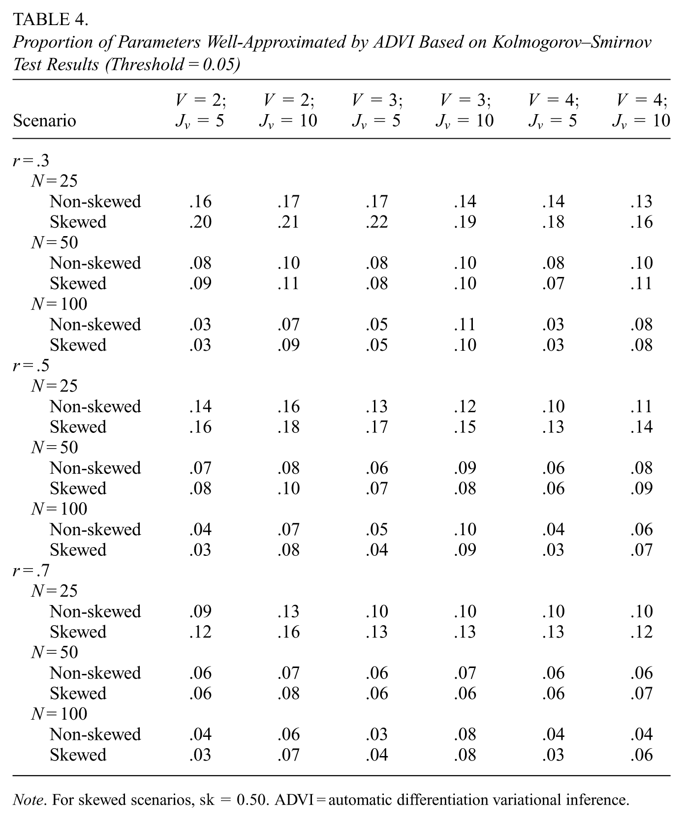
Note. For skewed scenarios,
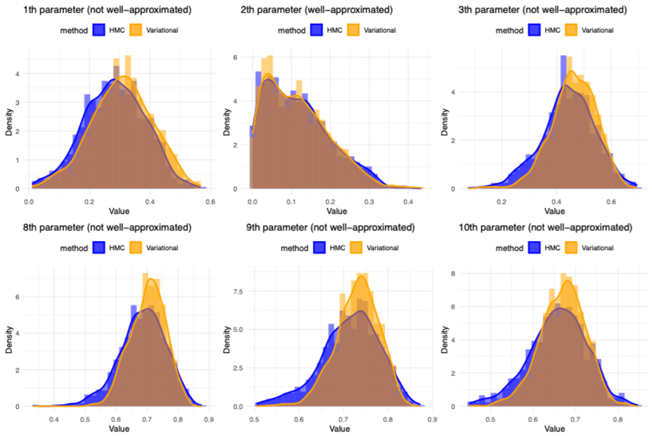
Comparison of posterior distributions: HMC versus ADVI (one simulation with
Empirical Study: Application to TIMSS Grade 8 Mathematics Student Questionnaire
Having established the performance of our Bayesian parameter estimation methods (HMC and ADVI) in simulated data, we applied these methods to real data from the 2019 TIMSS Grade 8 Mathematics Student Questionnaire (TIMSS & PIRLS International Study Center, 2019). This application serves to validate our proposed methods in a real-world context, where factors such as sample variability, missing data, and expert priors introduce additional complexities.
TIMSS 2019 is a large-scale international assessment of mathematics and science at Grades 4 and 8, administered to nationally representative samples across 64 countries and 8 benchmarking participants. Typical national samples included ~4,000 students per grade drawn from ~150 to 200 schools, resulting in approximately 330,000 Grade 4 and 250,000 Grade 8 students worldwide. Alongside the mathematics and science tests, TIMSS 2019 collects student questionnaire data covering attitudinal, behavioral, and background variables.
Data and Model Specification
The 2019 TIMSS Grade 8 Mathematics Student Questionnaire includes a wide range of background and attitudinal items designed to capture students’ engagement with mathematics learning. In particular, we focused on 27 Likert-type items (with four response categories) that measure three key dimensions of engagement: (a) confidence in learning mathematics—belief in one’s ability to succeed in mathematics; (b) enjoyment of learning mathematics—general interest and positive attitude toward mathematics; (c) value of learning mathematics—perceived importance of mathematics for future academic and career opportunities.
To reflect real-world classroom contexts, we randomly selected 10 small samples, each consisting of approximately 25 U.S. students, from the 2019 TIMSS dataset. Based on our previous findings, we gathered expert ratings from 12 eighth-grade mathematics teachers to serve as prior knowledge in our Bayesian approach. These teachers, recruited from various schools in Boston and Texas, evaluated each item’s relevance to its intended dimension using a four-point scale.
Parameter Estimation Results
For the CFA benchmark, we used the full U.S. Grade 8 sample of TIMSS 2019, which consists of 8,698 students who completed the mathematics student questionnaire. Given this large sample size, CFA estimates are stable and can reasonably be treated as “true” parameter values for benchmarking the performance of our Bayesian estimation methods. The item-to-dimension correlations were generally high, with most exceeding .80, confirming the strong construct validity of the TIMSS instrument. When applying our Bayesian estimation methods to the small samples, results (Table 5) corroborate our earlier findings for instruments with three dimensions and 10 items per dimension:
CFA produced out-of-bound estimates when sample sizes were as small as 25.
ADVI outperformed HMC in estimating item-to-dimension correlations
HMC sampling is all well-mixed when using priors derived from 12 experts’ ratings.
Comparison of MSEs Across Three Methods for Estimating
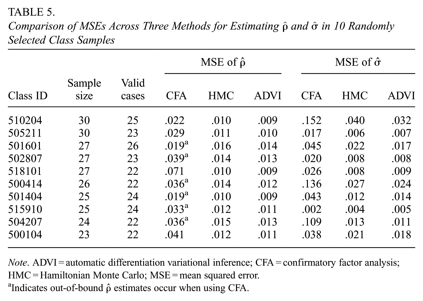
Note. ADVI = automatic differentiation variational inference; CFA = confirmatory factor analysis; HMC = Hamiltonian Monte Carlo; MSE = mean squared error.
Indicates out-of-bound
A notable challenge arose in setting expert-informed priors. Cohen’s (1988) conventional cut-points were insufficient for capturing the high correlations observed in the real data. Even when all 12 experts rated an item as “Highly relevant” (i.e., a rating of 4), the prior mean for
This adjustment is reasonable for the following reasons. First, Cohen’s original cut-points are intentionally broad; the interval for “Highly relevant” spans ρ ∈ (0.50, 1.0), which does not align well with the narrow range of high correlations observed here. Second, the TIMSS 2019 questionnaire is a production-quality instrument that has undergone extensive development and screening, leaving items with consistently strong item–trait correlations (often near .90). In contrast, during an instrument development stage, where weaker items remain, Cohen’s thresholds may be more appropriate. Third, a natural long-term solution may be to refine Cohen’s scale by introducing a fifth category, distinguishing between “Highly relevant” (e.g., ρ ∈ (0.50, 0.80)) and “Extremely relevant” (e.g., ρ ∈ (0.80, 1.0)). Such an extension would better accommodate mature instruments while preserving applicability in early-stage development contexts.
Discussion and Conclusion
This study introduced a novel Bayesian framework for establishing validity evidence in multi-unidimensional instruments under small-sample conditions. By integrating expert-informed priors into a Bayesian parameter estimation procedure—and leveraging advanced sampling techniques such as HMC and ADVI—we addressed the limitations of traditional ordinal CFA when sample sizes are restricted. Extensive simulation studies and an empirical application using TIMSS Grade 8 Mathematics data provided critical insights into our approach.
We first demonstrated that incorporating expert-informed priors significantly improves parameter estimation accuracy in small-sample settings. Traditional CFA struggled under these conditions, often producing out-of-bound estimates and high MSEs. By contrast, our Bayesian approach, incorporating priors from
Next, we compared HMC and ADVI with respect to estimation accuracy, computational efficiency, and approximation quality. Table 3 shows that ADVI consistently performs better than HMC for item-to-dimension correlations (
When comparing runtimes, ADVI showed a pronounced advantage in computational efficiency, requiring far less processing time than HMC. This gap widened as sample size, dimensionality (
When deciding between HMC and ADVI, researchers should consider both the goals of their analysis and practical constraints. ADVI is generally the better choice when estimating item-to-dimension correlations (
Limitations and Future Research
Despite the promising results and practical contributions of this research, several limitations and potential directions for future work warrant discussion.
First, this study focused on multi-unidimensional instruments with up to four dimensions and 10 items per dimension. Although these designs represent many practical assessment scenarios, they do not encompass more complex structures (e.g., multidimensional or hierarchical models). Extensions of the current Bayesian approach to accommodate such advanced measurement frameworks could provide deeper insights into its versatility and performance.
Second, a key feature of our Bayesian approach is the incorporation of expert-informed priors. While the inclusion of expert knowledge can greatly enhance parameter estimation for small samples, the quality and consistency of these expert ratings proved critical. Our simulations and empirical findings both revealed that coarse rating scales (e.g., 1–4) often fail to capture high correlations reliably, leading to biases. Future research could explore the use of more granular rating scales (e.g., 1–5 or continuous sliders) and provide additional training to improve rater accuracy and consistency.
Third, while HMC remains the “gold standard” for capturing intricate posterior dependencies, its computational overhead rises rapidly with increasing number of dimensions, items, or sample sizes. Investigating more efficient sampling algorithms could help strike a balance between accuracy and runtime.
Lastly, although ADVI demonstrated significant speed advantages and performed well for item-level parameters (
Supplemental Material
sj-docx-1-jeb-10.3102_10769986251393420 – Supplemental material for A Bayesian Framework to Establish Validity Evidence for Multi-Unidimensional Instruments With Small Samples
Supplemental material, sj-docx-1-jeb-10.3102_10769986251393420 for A Bayesian Framework to Establish Validity Evidence for Multi-Unidimensional Instruments With Small Samples by Jihang Chen and Zhushan Li in Journal of Educational and Behavioral Statistics
Footnotes
Appendix A: Hamiltonian Monte Carlo
Hamiltonian Monte Carlo (HMC) simulates Hamiltonian dynamics to explore posterior distributions efficiently. The Hamiltonian function is defined as
where
The evolution of the system follows Hamilton’s equations:
To numerically approximate these continuous dynamics, HMC employs the leapfrog method:
After multiple steps, the proposed state (
If a uniform random variable
Appendix B: Automatic Differentiation Variational Inference
Automatic differentiation variational inference (ADVI) approximates the posterior
A common choice for the variational family is a diagonal Gaussian:
where
The ELBO is computed as
where
To maximize the ELBO, ADVI uses stochastic gradient descent with the following techniques:
Declaration of Conflicting Interests
The authors declared no potential conflicts of interest with respect to the research, authorship, and/or publication of this article.
Funding
The authors received no financial support for the research, authorship, and/or publication of this article.
Notes
Authors
References
Supplementary Material
Please find the following supplemental material available below.
For Open Access articles published under a Creative Commons License, all supplemental material carries the same license as the article it is associated with.
For non-Open Access articles published, all supplemental material carries a non-exclusive license, and permission requests for re-use of supplemental material or any part of supplemental material shall be sent directly to the copyright owner as specified in the copyright notice associated with the article.