A Restricted Latent Class Hidden Markov Model for Polytomous Responses,Polytomous Attributes,and Covariates: Identifiability and Application

Abstract

We introduce a restricted latent class exploratory model for longitudinal data with ordinal attributes and respondent-specific covariates. Responses follow a time-inhomogeneous hidden Markov model where the probability of a respondent’s latent state at the current time point is conditional on the respondent’s latent state at the previous time point as well as the respondent’s covariates at the current time point. We prove that the model is identifiable, state a Bayesian formulation, and demonstrate its efficacy in a variety of scenarios through two simulation studies. We apply the model to response data from a mathematics examination, comparing the results to a previously published confirmatory analysis, and also apply it to emotional state response data, which was measured over a several-day period.

Keywords

Bayesian inference hidden Markov model longitudinal multivariate probit restricted latent class model

1 Introduction

Latent class models (Goodman, 1974) are an exploratory method of classifying respondents into a finite set of latent or unobserved classes, under the assumption that responses are conditionally independent given the class membership of respondents. Restricted latent class models (RLCMs; E. Haertel, 1984; E. H. Haertel, 1990; Vermunt, 2001) are a type of latent class model where the restrictions on certain parameters allow for an interpretation of the relationship between the response data and the latent state of the respondents. The discrete aspect of these latent states makes RLCMs useful in settings where classification of the latent state can serve the purpose of finding values of latent attributes with an interpretation that is of interest to the researcher and respondents.

A major type of model where latent class membership is modeled over time is the hidden Markov model (Baum & Petrie, 1966; Wiggins, 1955). In the literature, a specific type of hidden Markov model that has been used to model latent class membership over time is referred to by the name “latent transition analysis” (Collins & Wugalter, 1992; Hagenaars, 1990; Poulsen, 1983; van de Pol & Langeheine, 1990). A hidden Markov model has three components: the emission probabilities, which are the probabilities of response values conditional on the value of the latent state, the transition probabilities between time points, which are the probabilities of latent state values at a time point conditional on the latent state value at the previous time point, and the marginal probability of the latent state at the initial time point (Miller, 2016). Several latent class models for which the transition model is a hidden Markov model have been introduced. Wang et al. (2018) introduced a model with binary attributes that models the transition matrix as a function of covariates. Y. Chen et al. (2018) presented a model that uses a categorical distribution over the number of possible trajectories. In the model of Zhang and Chang (2020), interventions are related to the changes in the latent state. Li et al. (2016) and Kaya and Leite (2017) use the deterministic-input noisy-and-gate (DINA) model and both the DINA and the deterministic input noisy-or-gate model (DINO) models respectively as measurement models in a latent transition analysis framework. The R package TDCM (Madison et al., 2025) provides functionality for fitting the transition diagnostic classification model (Madison & Bradshaw, 2018), a confirmatory model (where the latent structure is prespecified) with binary attributes and binary data.

Two relevant longitudinal models which do not fit into the hidden Markov model framework are that of Y. Chen and Culpepper (2020), for which the probability of each latent state is conditional on shared parameters and where the latent state is modeled by a multivariate probit specification, and that of Bartolucci and Farcomeni (2009), which is a longitudinal model for polytomous data with random effects that take on discrete values.

We consider latent class models in which the latent classes arise from vectors where each component is a level of a latent attribute. Much of the previous work of this type of RLCM utilized binary latent attributes. When performing a diagnosis, attributes with multiple levels (polytomous attributes) allow for a richer description of a condition or knowledge state. A concept utilized by some models of this type is the $Q$ -matrix (Rupp et al., 2010). $Q$ -matrices specify a relationship between the latent state and the response values: they enter models in a manner similar to variable selection matrices. The particular form the $Q$ -matrix takes depends on the model being specified.

There has been work on models that utilize polytomous attributes. J. Chen and de la Torre (2013) introduced a model where the attributes are expert-defined. In the model of Sun et al. (2013), the attributes have particular levels relating to a polytomous $Q$ -matrix. The models of He et al. (2023) and Wayman et al. (2025) both introduced RLCMs which are similar to the model presented in this manuscript, but are only for the cross-sectional setting. The model presented in Chapter 5 of Bartolucci et al. (2012) is similar to the model we introduce here, but our model uses a multivariate probit specification for the transition model which incorporates covariates through the mean of the underlying continuous random vector, a parameterization not included there.

Regarding identifiability, J. Liu et al. (2013) established identifability for a cross-sectional model with binary attributes and binary responses that uses a $Q$ -matrix. Xu (2017) and Xu and Shang (2018) established identifiability for a cross-sectional model with binary attributes, binary responses, a particular monotonicity condition, and a $Q$ -matrix that satisfies certain conditions. More recently, Y. Liu et al. (2023) established the identifiability of a longitudinal model with binary responses, binary attributes whose transition probabilities follow a hidden Markov model, and a $Q$ -matrix satisfying certain conditions.

This paper introduces an RLCM where latent states consisting of polytomous attributes change over time and where covariates can help explain transitions amongst components of the latent attribute vectors. We do this by extending to the longitudinal setting of the RLCM of Wayman et al. (2025) for cross-sectional data, where respondent-specific covariates are related to the respondent’s latent state through a multivariate probit model. Our model uses a restricted hidden Markov model to uncover structure in the attribute change process: observed responses occur with a probability conditional on the value of a latent variable (the emissions probabilities) and the transition probabilities for each latent state value are conditional only on the previous time point. Just as exploratory restricted latent class models have proven useful for diagnostic models by finding structure in general finite mixture models in the cross-sectional setting, when we move to the longitudinal setting, we have an analogous benefit in finding greater structure in hidden Markov models.

Compared to some previous models, ours is exploratory rather than confirmatory. We demonstrate in our education application that this exploratory model improves upon the best confirmatory model (Tang & Zhan, 2021) for a particular dataset (Zhan, 2021) measuring performance on a mathematics assessment and the effectiveness of a particular intervention. That model, the sLong-DINA, has a unidimensional higher order factor, whereas our model utilizes a multivariate probit whose correlation matrix can capture more associations amongst the latent attributes. Combined with the fact that the $Q$ -matrix is not prespecified, this leads to a more accurate representation of the underlying attributes and how they relate to performance.

The structure of this paper is as follows. We first outline the main components of the model, and then state a Bayesian formulation of the model from whose posterior we can sample. We then show that the model is identifiable. Next, we describe the sampling algorithm, which makes use of parameter expansion. We display simulation results which demonstrate the accuracy of parameter estimation in a variety of scenarios. We then apply the model to two different sets of longitudinal data: data that were gathered as part of an education study, and data that were gathered to study respondents’ emotional states over time. We conclude with a discussion.

2 Methodology

In the following, for any $S \in N$ , let $[S]$ denote the set ${1, 2, \dots, S}$ , and for any matrix $A$ let $A^{'}$ denote the transpose of $A$ . We observe the responses of $N$ respondents at $T$ time points to the same questionnaire of $J$ questions with ordinal responses (also referred to as items); we denote the response of respondent $n$ at time point $t$ as $Y_{n}^{t} = (Y_{n 1}^{t}, \dots, Y_{nJ}^{t})$ , where for each $j \in [J]$ we have $Y_{nj}^{t} \in {0, 1, \dots, M_{j} - 1}$ . We also observe a respondent-specific vector of $D$ covariates, denoted $X_{n}^{t} \in R^{1 \times D}$ . We assume each respondent has a $K$ -dimensional latent state (also referred to as the attribute profile) at each time point $t$ , which we denote as $α_{n}^{t} = (α_{n 1}^{t}, \dots, α_{nK}^{t}) \in {0, \dots, L - 1}^{K} = : A_{L}$ , where $L$ is a fixed natural number.

As a time-inhomogeneous (Seneta, 2006) hidden Markov model, our model includes both an emissions matrix, here a matrix of latent state-conditional item response probabilities which is the same for all respondents and all time points, as well as a set of transition matrices between all time points and a vector of probabilities for the latent state at the initial time point, both of which can vary across time points and across respondents. We denote the $(\sum_{j = 1}^{J} M_{j}) \times L^{K}$ emissions matrix by $B = (p (Y_{n}^{t} ∣ α_{n}^{t}, θ_{m}))$ (this matrix is the same for all $n$ and all $t$ ). This component of the model is the measurement model and we thus denote its parameters as $θ_{m}$ .

We write the $L^{K} \times L^{K}$ transition matrix for respondent $n$ from time $t - 1$ to time $t$ as $U_{n, t, t - 1} = (p (α_{n}^{t} ∣ α_{n}^{t - 1}, θ_{s}))$ , and the vector of marginal probabilities (of dimension $L^{K}$ ) for the latent state of respondent $n$ at time $t$ as $π_{n}^{t} = (p (α_{n}^{t} ∣ θ_{s}))$ . The set of transition matrices for all $n$ for $t \in {2, \dots, T}$ and the initial latent state probabilities for all $n$ at $t = 1$ form the structural model, so we denote the parameters relevant to these components as $θ_{s}$ .

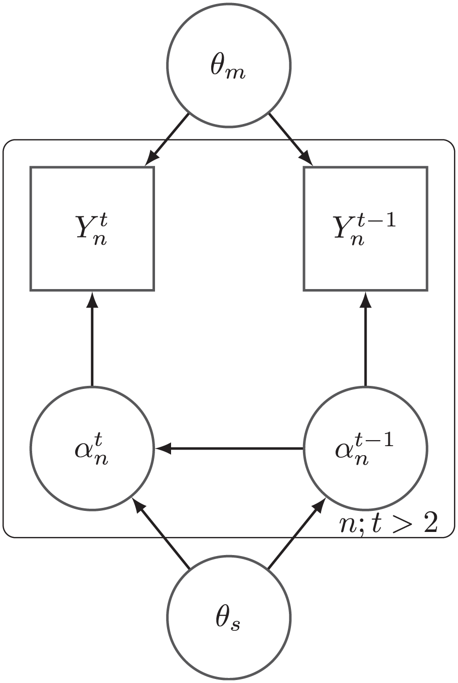
We now describe the components of the model, namely the measurement model, structural model, and a monotonicity condition regarding the latent state and the response data. A simplified version of the model is shown in Figure 1 in directed graphical model form (Murphy, 2012).

Figure 1.

Simplified version of the model in directed graphical model form (for alt text, see Supplemental Material A in the online version of the journal).

2.1 Measurement Model

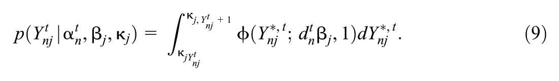
The measurement model forms the elements of the emissions matrix $B = (p (Y_{n}^{t} ∣ α_{n}^{t}, θ_{m}))$ . It is a cumulative probit link model (Agresti, 2015), namely, for all $n \in [N]$ , $t \in [T]$ , $j \in [J]$ and $m \in {0, \dots, M_{j} - 1}$ ,

p (Y_{nj}^{t} = m ∣ α_{n}^{t}, θ_{m}) = p (Y_{nj}^{t} = m ∣ α_{n}^{t}, β_{j}, κ_{j}) = Φ (κ_{j, m + 1} - d_{n}^{t} β_{j}) - Φ (κ_{j, m} - d_{n}^{t} β_{j})

(1)

where $θ_{m} = (κ, β)$ , $Φ$ denotes the cdf of the standard normal distribution, where for each $j$ , $κ_{j 0} < κ_{j 1} < \dots < κ_{j M_{j}}$ and $κ_{j 0} = - \infty, κ_{j 1} = 0, κ_{j M_{j}} = \infty$ for identifiability reasons, and where $d_{n}^{t}$ is a function of $α_{n}^{t}$ and is called the design vector of respondent $n$ .

We use a cumulative coding (He et al., 2023; Wayman et al., 2025) of $α_{n}^{t}$ in order to relate the effect of potentially each level and dimension of $α_{n}^{t}$ to the observed response $Y_{nj}^{t}$ . Specifically, for $α_{n}^{t} = (α_{n 1}^{t}, \dots, α_{nK}^{t})$ we define, for all $k \in [K]$ , the functions $d_{k} : A_{L} \to {0, 1}^{L}$ by $d_{k} (α_{n}^{t}) = (I (α_{nk}^{t} \geq 0), I (α_{nk}^{t} \geq 1), \dots, I (α_{nk}^{t} \geq L - 1))$ . We define the function

d : A_{L} \to {0, 1}^{Π_{k = 1}^{K} L}

(2)

by $d (α_{n}^{t}) = d_{1} (α_{n}^{t}) \otimes d_{2} (α_{n}^{t}) \otimes \dots \otimes d_{K} (α_{n}^{t})$ , and we write the value of $d$ evaluated at $α_{n}^{t}$ as $d_{n}^{t}$ . Our definition for $d_{n}^{t}$ corresponds with the saturated model that includes all main effects and interaction terms. We may fit reduced models by only using a subset of components of the design vector, which includes only the interactions we desire. For example, reduced models might only include main effects (order $1$ ), or main effects and two-way interactions (order $2$ ), potentially up to a saturated model of order $K$ .

2.2 Monotonicity Condition

For two arbitrary $u, v \in A_{L}$ , $u = (u_{1}, \dots, u_{K})$ and $v = (v_{1}, \dots, v_{K})$ , we write $u \geq v$ if for all $k \in [K]$ we have $u_{k} \geq v_{k}$ .

So that our ordinal latent state vectors have an interpretation related to observable ordinal quantities, we impose a monotonicity condition used in earlier models (Culpepper, 2019; Wayman et al., 2025): for all $t \in [T]$ , $n \in [N]$ , and $t \in [T]$ ,

\forall u, v \in A_{L} u \geq v \Rightarrow p (Y_{nj}^{t} > m ∣ u, β_{j}, κ_{j}) \geq p (Y_{nj}^{t} > m ∣ v, β_{j}, κ_{j}),

(3)

equivalently, for all $u, v \in A_{L}, u \geq v \Rightarrow d_{u} β_{j} \geq d_{v} β_{j}$ (where $d_{u}$ is the design vector associated with $u$ ). This monotonicity condition restricts the parameter space for $β_{j}$ .

2.3 Structural Model

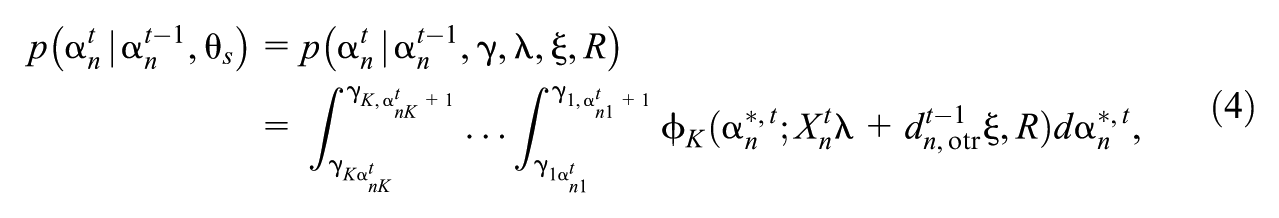
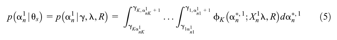
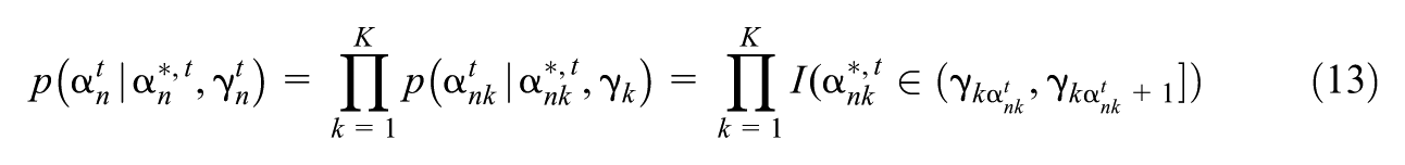
The structural model forms the transition matrices, that is, for $t \in {2, 3, \dots, T}$ , $U_{n, t, t - 1} = (p (α_{n}^{t} ∣ α_{n}^{t - 1}, θ_{s}))$ , as well as the initial latent state probabilities $π_{n}^{t} = (p (α_{n}^{t} ∣ θ_{s}))$ for $t = 1$ . The structural model is a multivariate probit model (Ashford & Sowden, 1970; Christoffersson, 1975; McDonald, 1967; Muthén, 1978) where for $t \in {2, \dots, T}$ , the latent state at time point $t$ , $α_{n}^{t}$ , is related to its value at time point $t - 1$ as well as the covariates $X_{n}^{t}$ through the mean of an underlying multivariate normal random variable, namely

\begin{matrix} p (α_{n}^{t} ∣ α_{n}^{t - 1}, θ_{s}) = p (α_{n}^{t} ∣ α_{n}^{t - 1}, γ, λ, ξ, R) \\ = \int_{γ_{K α_{nK}^{t}}}^{γ_{K, α_{nK}^{t} + 1}} \dots \int_{γ_{1 α_{n 1}^{t}}}^{γ_{1, α_{n 1}^{t} + 1}} ϕ_{K} (α_{n}^{*, t}; X_{n}^{t} λ + d_{n, otr}^{t - 1} ξ, R) d α_{n}^{*, t}, \end{matrix}

(4)

where $θ_{s} = (γ, λ, ξ, R)$ , where $ϕ_{K} (x; a, b)$ is the density function of a multivariate normal random variable of dimension $K$ in which $x$ is the variable (row vector), $a$ is the mean, and $b$ is the covariance, and where $d_{n, otr}^{t}$ is the design vector for the structural model with order otr (where otr stands for “order of transition model”). For each $k \in [K]$ , we assume $γ_{k 0} < γ_{k 1} < \dots < γ_{kL}$ , where we set $γ_{k 0} = - \infty$ , $γ_{k 1} = 0$ , and $γ_{kL} = \infty$ for identifiability.

For $t = 1$ , we assume

p (α_{n}^{1} ∣ θ_{s}) = p (α_{n}^{1} ∣ γ, λ, R) = \int_{γ_{K α_{nK}^{1}}}^{γ_{K, α_{nK}^{1} + 1}} \dots \int_{γ_{1 α_{n 1}^{1}}}^{γ_{1, α_{n 1}^{1} + 1}} ϕ_{K} (α_{n}^{*, 1}; X_{n}^{1} λ, R) d α_{n}^{*, 1}

(5)

We choose a correlation structure rather than a covariance structure for identifiability reasons (see Section 4 and Supplemental Material E in the online version of the article).

We now detail the Bayesian model we implement that reflects the above components.

3 Bayesian Model

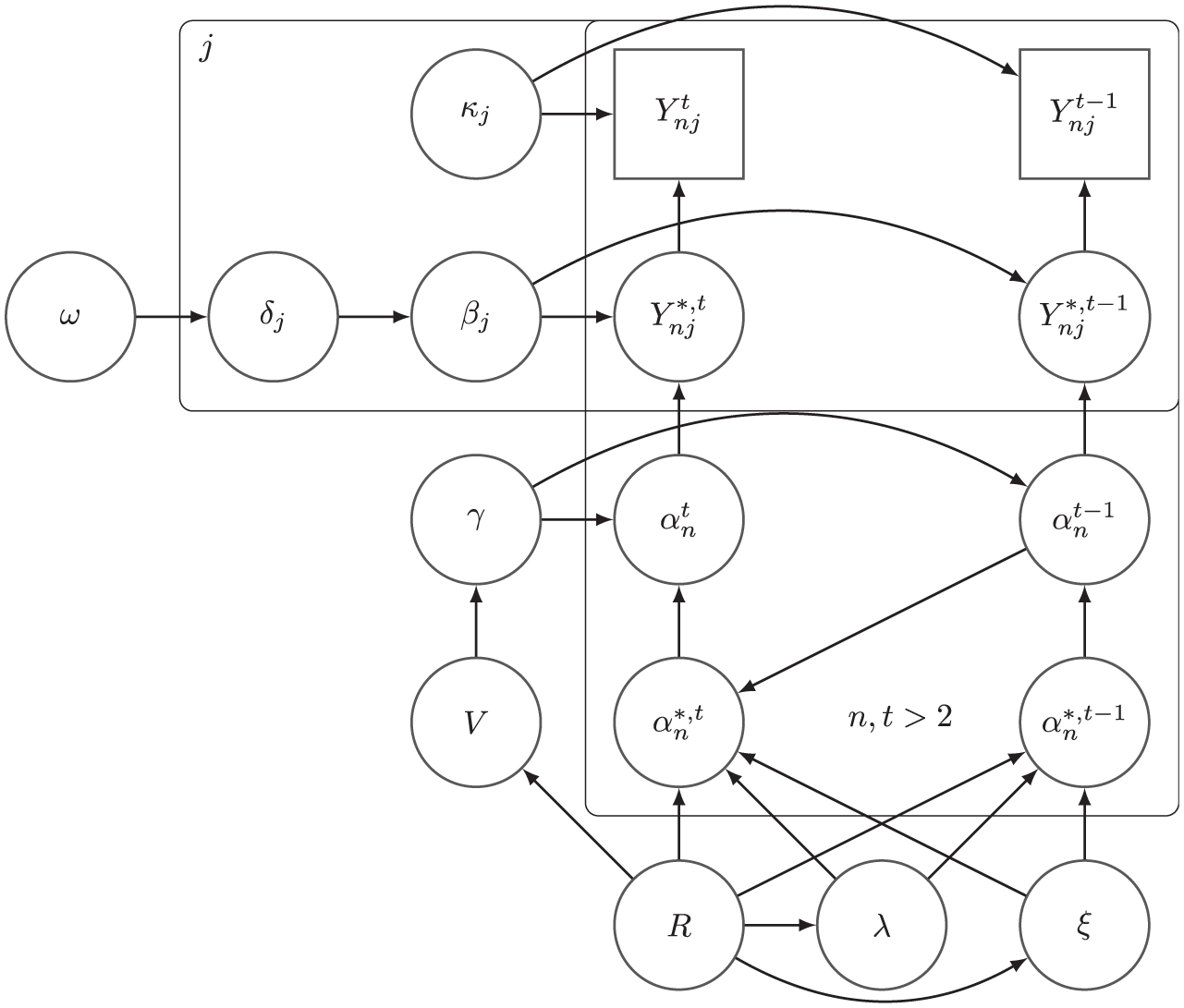
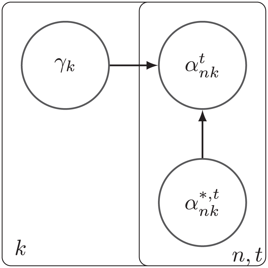
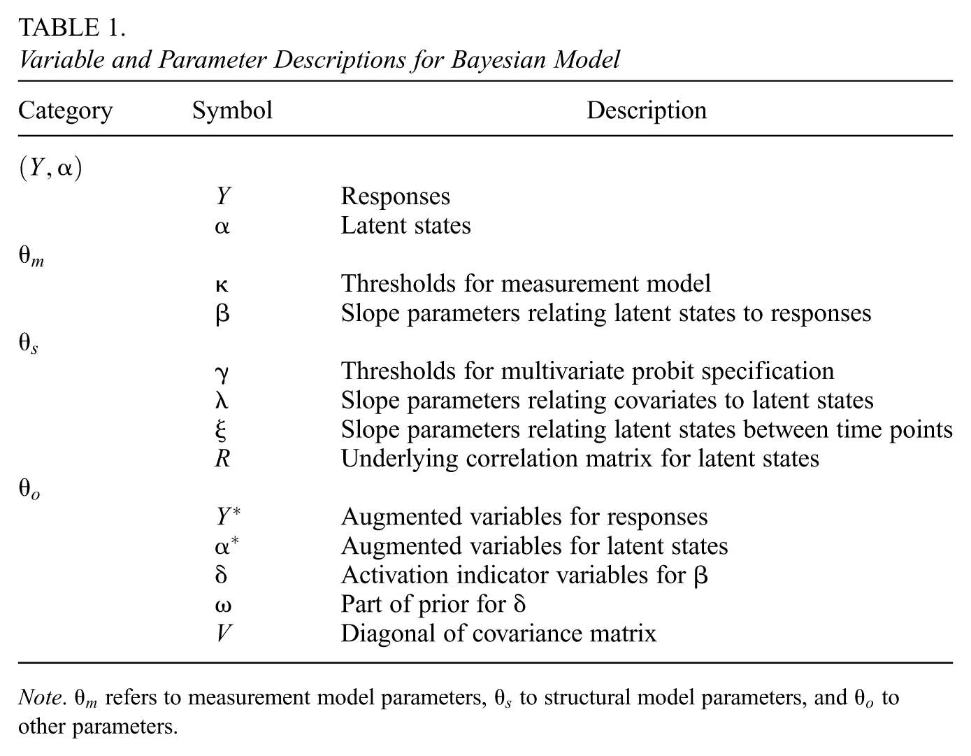
Our Bayesian model is formulated as a directed graphical model (Murphy, 2012), the graph $G$ for which is displayed in Figures 2 and 3 using plate notation (Murphy, 2012). We label the set of vertices in $G$ as $Z = (Y, α, θ, θ_{o})$ , where $θ = (θ_{m}, θ_{s})$ is the set of measurement model parameters $θ_{m}$ and structural model parameters $θ_{s}$ , and $θ_{o}$ denotes other parameters introduced for computational purposes; the variables and parameters are listed in Table 1. Parameters with an asterisk superscript are present for computational purposes.

Figure 2.

Bayesian model in directed graphical model form, part one (for alt text, see Supplemental Material A in the online version of the journal).

Figure 3.

Bayesian model in directed graphical model form, part two (for alt text, see Supplemental Material A in the online version of the journal).

Table 1.

Variable and Parameter Descriptions for Bayesian Model

Category Symbol	Description
$(Y, α)$
$Y$	Responses
$α$	Latent states
$θ_{m}$
$κ$	Thresholds for measurement model
$β$	Slope parameters relating latent states to responses
$θ_{s}$
$γ$	Thresholds for multivariate probit specification
$λ$	Slope parameters relating covariates to latent states
$ξ$	Slope parameters relating latent states between time points
$R$	Underlying correlation matrix for latent states
$θ_{o}$
$Y^{*}$	Augmented variables for responses
$α^{*}$	Augmented variables for latent states
$δ$	Activation indicator variables for $β$
$ω$	Part of prior for $δ$
$V$	Diagonal of covariance matrix

Note. $θ_{m}$ refers to measurement model parameters, $θ_{s}$ to structural model parameters, and $θ_{o}$ to other parameters.

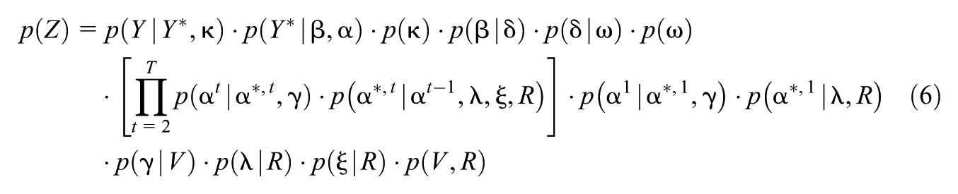
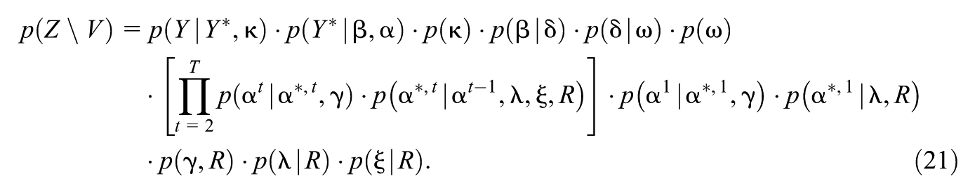
Since our model $p (Z)$ is a directed graphical model (Murphy, 2012) it “admits a recursive factorization according to $G$ ” (Lauritzen, 1996), that is, $p (Z) = \underset{z \in Z}{Π} p (z ∣ pa (z))$ where $pa (z)$ refers to the parents of vertex $z$ .

From the recursive factorization, we have

\begin{matrix} p (Z) = p (Y ∣ Y^{*}, κ) \cdot p (Y^{*} ∣ β, α) \cdot p (κ) \cdot p (β ∣ δ) \cdot p (δ ∣ ω) \cdot p (ω) \\ \cdot [Π_{t = 2}^{T} p (α^{t} ∣ α^{*, t}, γ) \cdot p (α^{*, t} ∣ α^{t - 1}, λ, ξ, R)] \cdot p (α^{1} ∣ α^{*, 1}, γ) \cdot p (α^{*, 1} ∣ λ, R) \\ \cdot p (γ ∣ V) \cdot p (λ ∣ R) \cdot p (ξ ∣ R) \cdot p (V, R) \end{matrix}

(6)

where we have taken the additional step of writing $p (V ∣ R) \cdot p (R) = p (V, R)$ . Note that we have grouped across subscripts.

Since the model is a directed graphical model, it obeys the directed local Markov property (Lauritzen, 1996) relative to $G$ , that is, for any variable $z \in Z$ we have $z ╨ nd (z) ∣ pa (z)$ where $nd (z)$ denotes the non-descendants of $z$ . Note that this implies $z ╨ (nd (z) ∖ pa (z)) ∣ pa (z)$ .

We now specify assumed relationships (likelihood, priors) for factors that appear in Equation 6.

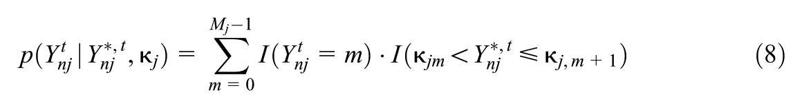
3.1 Likelihood and Data Augmentation Prior for Observed Data

We assume for all $n \in [N]$ , $t \in [T]$ , and $j \in [J]$ ,

p (Y_{nj}^{*, t} ∣ α_{n}^{t}, β_{j}) = ϕ (Y_{nj}^{*, t}; d_{n}^{t} β_{j}, 1)

(7)

where $ϕ (x; a, b)$ is the normal density with variable $x$ , mean $a$ , and variance $b$ , and

p (Y_{nj}^{t} ∣ Y_{nj}^{*, t}, κ_{j}) = \sum_{m = 0}^{M_{j} - 1} I (Y_{nj}^{t} = m) \cdot I (κ_{jm} < Y_{nj}^{*, t} \leq κ_{j, m + 1})

(8)

which yields (see Supplemental Material B in the online version of the journal)

p (Y_{nj}^{t} ∣ α_{n}^{t}, β_{j}, κ_{j}) = \int_{κ_{{jY}_{nj}^{t}}}^{κ_{j, Y_{nj}^{t} + 1}} ϕ (Y_{nj}^{*, t}; d_{n}^{t} β_{j}, 1) {dY}_{nj}^{*, t} .

(9)

We assume $p (κ_{j}) = I (- \infty = κ_{j 0} < κ_{j 1} < \dots < κ_{jMj} = \infty)$ .

3.2 Priors for Measurement Model Coefficients and Related Parameters

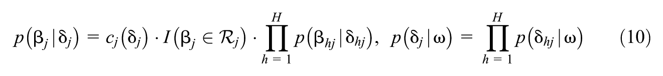
We use the Dirac spike and normal slab prior for variable selection (Kuo & Mallick, 1998) for each $β_{j}$ , namely, for all $j \in [J]$ :

p (β_{j} ∣ δ_{j}) = c_{j} (δ_{j}) \cdot I (β_{j} \in R_{j}) \cdot Π_{h = 1}^{H} p (β_{hj} ∣ δ_{hj}), p (δ_{j} ∣ ω) = Π_{h = 1}^{H} p (δ_{hj} ∣ ω)

(10)

p (β_{hj} ∣ δ_{j}) = p (β_{hj} ∣ δ_{hj}) = I (δ_{hj} = 0) \cdot Δ (β_{hj}) + I (δ_{hj} = 1) \cdot ϕ (β_{hj}; 0, σ_{β}^{2})

(11)

R_{j} : = {β_{j} \in R^{H} : \forall u, v \in A_{L} u \geq v \Rightarrow d_{u} β_{j} \geq d_{v} β_{j}}

(12)

where $δ_{hj} ∣ ω ~ Bernoulli (ω)$ , $Δ$ is the Dirac delta generalized function, and $R_{j}$ is the region reflecting the monotonicity condition (Equation 3). As in Y. Chen et al. (2020) and Wayman et al. (2025), we let $ω ~ Beta (ω_{0}, ω_{1})$ where $ω_{0}$ and $ω_{1}$ are hyper-parameters.

3.3 Priors for Structural Model Parameters

For all $n \in [N]$ and all $t \in [T]$ , we assume

p (α_{n}^{t} ∣ α_{n}^{*, t}, γ_{n}^{t}) = Π_{k = 1}^{K} p (α_{nk}^{t} ∣ α_{nk}^{*, t}, γ_{k}) = Π_{k = 1}^{K} I (α_{nk}^{*, t} \in (γ_{k α_{nk}^{t}}, γ_{k α_{nk}^{t} + 1}])

(13)

For all $n \in [N]$ and all $t \in {2, 3, \dots, T}$ , we assume

α_{n}^{*, t} ∣ λ, α_{n}^{t - 1}, ξ, R ~ N_{K} (X_{n}^{t} λ + d_{n, otr}^{t - 1} ξ, R)

(14)

and for $t = 1$ ,

α_{n}^{*, t} ∣ λ, R ~ N_{K} (X_{n}^{t} λ, R) .

(15)

These give (see Supplemental Material B in the online version of the journal) Equations 4 and 5. We write $ζ = (λ^{'}, ξ^{'})^{'} \in R^{(D + H_{otr}) \times K}$ so Equations 14 and 15 can be written more simply as

α_{n}^{*, t} ∣ λ, α_{n}^{t - 1}, ξ, R ~ N_{K} (W_{n}^{t} ζ, R)

(16)

where $W_{n}^{t} = (X_{n}^{t}, d_{n, otr}^{t - 1})$ for $t \in {2, 3, \dots, T}$ and $W_{n}^{t} = (X_{n}^{t}, O)$ for $t = 1$ . Writing $α^{*, t} = ({α_{1}^{*, t}}^{'}, \dots, {α_{N}^{*, t}}^{'})^{'}$ and $α^{*} = ({α^{*, 1}}^{'}, \dots, {α^{*, T}}^{'})^{'}$ , as well as $W^{t} = ({W_{1}^{t}}^{'}, \dots, {W_{n}^{t}}^{'})^{'}$ and $W = ({W^{1}}^{'}, \dots, {W^{T}}^{'})^{'}$ gives

α^{*} ∣ α^{1, \dots, T - 1}, λ, ξ, R ~ N_{TN, K} (W ζ, I_{TN} \otimes R)

(17)

(see Supplemental Material C in the online version of the journal).

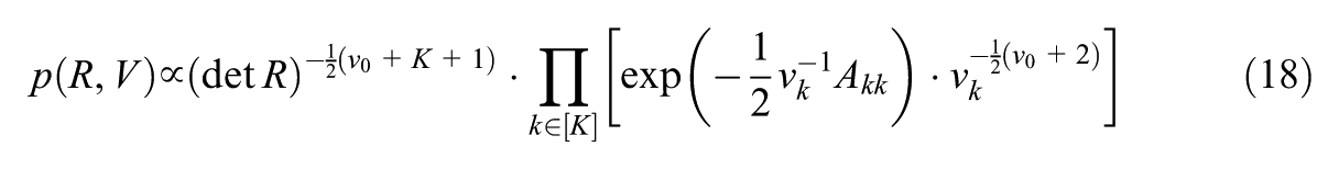
We decompose a positive definite covariance matrix $Σ$ as $V^{1 / 2} R V^{1 / 2}$ , where $V = diag (v_{1}, \dots, v_{K}) \in R^{K \times K}$ and for all $k \in [K]$ , $v_{k} > 0$ . For $p (R, V)$ , we use a prior from Wayman et al. (2025):

p (R, V) \propto (\det R)^{- \frac{1}{2} (v_{0} + K + 1)} \cdot \underset{k \in [K]}{Π} [\exp (- \frac{1}{2} v_{k}^{- 1} A_{kk}) \cdot v_{k}^{- \frac{1}{2} (v_{0} + 2)}]

(18)

where for all $k \in [K]$ , $A_{kk}$ are the diagonal elements of $R^{- 1}$ and $v_{0}$ is a hyperparameter.

For each $γ_{k}$ , we use a prior introduced in Wayman et al. (2025) for latent variable models with a discrete latent state, namely, for each level $l \in {2, 3, \dots, L - 1}$ , we assume $γ_{kl} ╨ γ_{k, l - 2}, γ_{k, l - 3}, \dots, γ_{k 3}, γ_{k 2} ∣ γ_{k, l - 1}, v_{k}$ so that

p (γ_{k} ∣ v_{k}) = p (γ_{k, L - 1} ∣ γ_{k, L - 2}, v_{k}) \cdot p (γ_{k, L - 2} ∣ γ_{k, L - 3}, v_{k}) \cdot \dots \cdot p (γ_{k 3} ∣ γ_{k 2}, v_{k}) \cdot p (γ_{k 2} ∣ v_{k})

(19)

and for each $l \in {2, 3, \dots, L - 1}$ we assume $γ_{kl} ∣ γ_{k, l - 1}, v_{k}$ follows a left-truncated exponential whose rate parameter $a$ is to be chosen such that the density is relatively flat:

p (γ_{k l} ∣ γ_{k, l - 1}, v_{k}) = I (γ_{k l} \in (γ_{k, l - 1}, \infty)) \cdot a v_{k}^{1 / 2} \cdot \exp [- a v_{k}^{1 / 2} \cdot (γ_{k l} - γ_{k, l - 1})] .

(20)

We let $λ ∣ R ~ N_{D, K} (0, I_{D} \otimes R)$ , and $ξ ∣ R ~ N_{H_{otr}, K} (0, I_{H_{otr}} \otimes R)$ , where $N_{N, K} (A, B \otimes C)$ indicates a matrix variate normal distribution (see Supplemental Material D in the online version of the journal) with mean $A$ and covariance matrix $B \otimes C$ . It follows that $ζ ∣ R ~ N_{D + H_{otr}, K} (0, I_{D + H_{otr}} \otimes R)$ .

3.4 Integrability of the Model with Respect to the Variance Parameter

By the directed local Markov property, $γ ╨ R ∣ V$ , so $p (γ ∣ V) \cdot p (R, V) = p (γ, R, V)$ . If we use this in Equation 6, we observe that $V$ does not appear on the right-hand side of any conditional bars, so integration with respect to $V$ is straightforward and gives

\begin{matrix} p (Z ∖ V) = p (Y ∣ Y^{*}, κ) \cdot p (Y^{*} ∣ β, α) \cdot p (κ) \cdot p (β ∣ δ) \cdot p (δ ∣ ω) \cdot p (ω) \\ \cdot [Π_{t = 2}^{T} p (α^{t} ∣ α^{*, t}, γ) \cdot p (α^{*, t} ∣ α^{t - 1}, λ, ξ, R)] \cdot p (α^{1} ∣ α^{*, 1}, γ) \cdot p (α^{*, 1} ∣ λ, R) \\ \cdot p (γ, R) \cdot p (λ ∣ R) \cdot p (ξ ∣ R) . \end{matrix}

(21)

4 Model Identifiability

Definition 1. For sets $A, B$ and an equivalence relation $~_{E}$ on $A$ , we say that $A$ is identifiable from $B$ up to $~_{E}$ if and only if there exists a surjective function $g : A \to B$ such that

\forall a, \tilde{a} \in A [g (a) = g (\tilde{a}) \Rightarrow a ~_{E} \tilde{a}]

(22)

Often $B$ is a family of density or likelihood functions and $A$ is a parameter space. In this situation, for readability we will often write ${f (Y ∣ θ)}$ to represent ${f_{Y} (• ∣ θ); θ \in Θ}$ . We state the definitions of two types of identifiability specifically for this situation.

Definition 2. For a discrete random variable $Y$ taking values on data space $Y$ and with ${f (Y ∣ θ)}$ a family of likelihoods or densities for $Y$ , $Θ$ is strictly identifiable from ${f (Y ∣ θ)}$ up to an equivalence relation $~_{E}$ if and only if

\forall θ, \tilde{θ} \in Θ [\forall y \in Y f_{Y} (y ∣ θ) = f_{Y} (y ∣ \tilde{θ})] \Rightarrow θ ~_{E} \tilde{θ} .

(23)

Definition 3. Let $N_{Λ}$ denote the family of all $Λ$ -null sets on the parameter space $Θ$ , where $Λ$ denotes the Lebesgue measure. For a discrete random variable $Y$ taking values on data space $Y$ and with ${f (Y ∣ θ)}$ a family of likelihoods or densities for $Y$ , $Θ$ is generically identifiable from ${f (Y ∣ θ)}$ up to an equivalence relation $~_{E}$ if and only if

\exists N \in N_{Λ} \forall θ, \tilde{θ} \in Θ ∖ N [\forall y \in Y f_{Y} (y ∣ θ) = f_{Y} (y ∣ \tilde{θ})] \Rightarrow θ ~_{E} \tilde{θ} .

(24)

Note that in Definitions 2 and 3, the surjective function of Definition 1 is the parameterization map.

When we say a parametric model for a variable $Y$ and parameter space $Θ$ is strictly (generically) identifiable up to an equivalence relation, we mean that $Θ$ is strictly (generically) identifiable from ${f (Y ∣ θ)}$ up to an equivalence relation. Also when applying either of the definitions, if the specific equivalence relation is not mentioned, it should be assumed that the relation is the equality relation.

We will prove that if certain conditions hold, $Θ = (Θ_{s}, Θ_{m})$ is strictly identifiable up to label swapping from ${f (Y ∣ θ)}$ , and if a certain subset of those conditions holds, $Θ$ is generically identifiable up to label swapping from ${f (Y ∣ θ)}$ . The label swapping equivalence relation on $Θ$ referred to here is the permutation of the rows and/or columns of all relevant vector or matrix parameters in $Θ$ that correspond to a permutation of the dimensions of the latent state vector (for example, if the labels of $α_{n}^{t}$ are permuted, the rows of $β$ would have to be permuted as well since each row of $β$ corresponds to a particular interaction effect of the dimensions of $α_{n}^{t}$ , which have been permuted).

The formal statement of this result is as follows:

Theorem 1. Define the following conditions:

(C1) For all $n \in [N]$ and $t \in [T]$ , all elements of $π_{n}^{t}$ are greater than zero (this implies that $rank (diag (π_{n}^{t})) = L^{K}$ )

(C2) $\sum_{j = 1}^{J} M_{j} \geq L^{K}$ (the total number of item responses is greater than or equal to the number of possible latent states)

(C3) there exist subsets $J_{1}, J_{2}, J_{3}$ of items such that the ranks of the three resulting block matrices comprising the emissions matrix $B$ are all of rank $L^{K}$ (this implies that $rank (B) = L^{K}$ , i.e. $B$ has full column rank)

(C4) for all $n \in [N]$ and $t \in {2, 3, \dots, T}$ , $rank (U_{n, t, t - 1}) = L^{K}$ (i.e. $U_{n, t, t - 1}$ has full rank)

(C5) $N \geq D + H_{otr}$

(C6) for all $t \in [T]$ , $rank (W^{t}) = D + H_{otr}$ (i.e. $W^{t}$ has full column rank)

In addition, define two conditions on the $δ$ matrix:

(D1) $δ$ has for each attribute an active main effect on all levels of the attribute for at least two items

(D2) $δ$ has no interaction effects active

If conditions (C1) through (C6) and (D1) hold, then ${p (Y ∣ θ)}$ is generically identifiable up to label swapping, and if conditions (C1) through (C6) and (D1) and (D2) hold, then ${p (Y ∣ θ)}$ is strictly identifiable up to label swapping.

See Supplemental Material E (available in the online version of this article) for the proof. We note that as part of the proof of Theorem 1, we prove that the single time-point multivariate probit model is strictly identifiable.

5 Parameter Expansion and Algorithm

In order to produce a model from which we can easily sample using a multiple-block Metropolis-Hastings algorithm (Chib, 2011), we perform a transformation of $Z$ to $\tilde{Z}$ ; our algorithm will sample from the model $p_{\tilde{z}} (\tilde{z}) = p_{Z} (g^{- 1} (\tilde{z})) \cdot | \det J_{g^{- 1}} (\tilde{z}) |$ . This methodology fits into the category of “parameter expansion” (J. S. Liu & Wu, 1999) or “conditional augmentation” (Meng & Van Dyk, 1999).

We transform $Z$ to $\tilde{Z}$ , where $\tilde{α^{*}} = α^{*} V^{1 / 2}$ , $\tilde{γ} = γ V^{1 / 2}$ , $\tilde{ζ} = ζ V^{1 / 2}$ , and $Σ = V^{1 / 2} R V^{1 / 2}$ , similar to the cross-sectional model we are extending (Wayman et al., 2025) (see Supplemental Material F [available in the online version of this article] for details). Our Metropolis-within-Gibbs algorithm samples from $p (\tilde{Z})$ and transforms each sampled value using the inverse of the transformation to produce a sample from the original model. The sampling steps are shown in Supplemental Material G (available in the online version of this article).

6 Software

A Python package (Wayman, 2025) containing an implementation of the procedures for simulation, data analysis, and model selection described in this manuscript has been released under a FLO (free/libre/open) license and is available at https://github.com/ericwayman01/probitlcmlongit. We note that the sampling algorithm is mostly implemented using the Armadillo C++ library (Sanderson & Curtin, 2019, 2025). The data generating parameters for the simulations and relevant files for the data analyses are available at https://github.com/ericwayman01/probitlcmlongit_related. For the data sets that were used for the data analyses, please refer to the Data Availability Statement.

7 Simulation Studies

To investigate the efficacy of the model in a variety of scenarios, we performed two simulation studies: simulation study one has larger sample sizes ( $N = 250, 500, 1, 500, 3, 000$ ) and a smaller number of time points ( $T = 3$ ), and simulation study two uses smaller sample sizes ( $N = 125, 250, 500$ ) and a larger number of time points ( $T = 30$ ). Simulation study two also includes an examination of the performance of the model when a percentage of time points of data are missing. These choices for the two simulation studies roughly correspond to the two data applications we present in Section 8.

The simulations are set up as follows. For a given combination of $K$ and $L$ , we create items in sets of five such that each set satisfies one of the following conditions: (1) for each dimension of the latent state, a set of items is related to that dimension alone, and (2) for each pair of dimensions of the latent state, a set of items is related to the pair of dimensions. For $K = 2$ this gives 15 items, for $K = 3$ , 25 items, and for $K = 4$ , 45 items. The $δ$ and $β$ matrices are chosen such that these relationships hold.

In order for the algorithm to be able to classify respondents correctly in terms of their latent class values, there need to be appreciably different patterns of item response class-conditional probabilities across classes: values of $κ$ are generated such that this is the case. Our simulation contains two covariates, age and sex, and we generate $λ$ such that there is some contribution of both covariates to the value of $α_{n}^{t}$ . $ξ$ is chosen such that each dimension of $α_{n}^{t - 1}$ affects that same dimension of $α_{n}^{t}$ , but no dimensions act in any combination.

We have 15 combinations of values of $K, L$ , and $ρ$ (where $ρ$ is the value of the off-diagonal elements of the correlation matrix $R$ ), and thus 15 sets of parameters as described above. We evaluate how the model performs in terms of parameter recovery for multiple sample sizes: we generate data from the model, run the model, obtain parameter estimates, and compare these estimates to the data-generating parameter values (this last step of the procedure is described in a later paragraph).

In the simulations, we set hyper-parameters to the following values for all scenarios: $σ_{β}^{2} = 2.0$ , $ω_{0} = 0.5$ , and $ω_{1} = 0.5$ , and $a = 1, 000^{- 1}$ . We set $v_{0} = K + 1$ so that we have uniform priors for the correlations (Barnard et al., 2000; Gelman & Hill, 2007). We tuned $σ_{κ}^{2}$ for each sample size so that its acceptance rate was roughly 40%. For all scenarios, the order of the measurement model was set to 2, and the order of the transition model was set to 1. For both simulation studies, for each replication we use a burn-in period of 6,000 draws and a post burn-in phase of 10,000 draws.

To evaluate convergence of the model, for all scenarios and all replications we ran the Geweke test (Geweke, 1992) on each element of each matrix parameter. For every scenario, it is the case that for every element, fewer than 2% of the replications yield a test statistic that falls outside the 95% confidence interval, and for most parameters the percentage is either zero or close to it. In addition, we examined integrated autocorrelation time (IAT; J. Liu, 2008; McGibbon, 2015; Plummer et al., 2006) for a representative replication for each scenario. We found that most matrix and vector parameters had an average IAT of less than 10 (corresponding to effective sample sizes of greater than 1,000); for some scenarios $β$ had a higher IAT. We also examined trace plots for various elements of matrix parameters to confirm convergence visually as we settled on a sufficient chain length.

In simulation study two, initial values for missing data rows were set as follows. In this simulation, each respondent $n$ has a known vector of time points for which $Y_{n}^{t}$ is missing, which is denoted $(t_{n}^{1}, \dots, t_{n}^{i})$ , $i \in [T]$ . For each respondent $n$ , if $t_{n}^{1} = 1$ we use the first value of data that is not missing that follows $t_{n}^{1}$ . Then, for any $t > 1$ for respondent $n$ , we proceed sequentially and for each $t$ use the first value of data that is not missing that precedes $t$ .

We evaluate parameter recovery on an element-wise basis. In addition to the parameters of the model, we report recovery of an additional “parameter,” $η$ , which is the set of class-conditional item response probabilities. For a given parameter (e.g., $β$ ), denote an element (e.g., $β_{hj}$ for some $h$ and $j$ ) for the moment by $θ$ , and denote by $θ^{(s, r)}$ the $s$ th draw of $θ$ from the Markov chain for the $r$ th replication in the post-burn-in phase. Letting $S$ be the number of draws in the post-burn-in phase, for elements of all parameters except $δ$ , we use the estimate of the posterior mean ${\hat{θ}}^{(r)} = (1 / S) \sum_{s = 1}^{S} θ^{(s, r)}$ ; for elements of $δ$ , we use the estimate of the posterior mode ${\hat{θ}}^{(r)} = I ((1 / S) \sum_{s = 1}^{S} θ^{(s, r)} > 0.5)$ . To measure how well parameters were recovered, for each replication we calculate a recovery metric: for elements of $γ, η, R, λ, ξ$ and $β$ , we calculate the absolute error of estimation for each element for replication $r$ , namely for a scalar $θ$ , ${AE}_{r} (θ, {\hat{θ}}^{(r)}) = | θ - {\hat{θ}}^{(r)} |$ . We then take the average of absolute error across all replications to arrive at the mean absolute error (MAE) for that element. For elements of $δ$ , we use correctness of estimation, namely for a scalar $θ$ , ${CE}_{r} (θ, {\hat{θ}}^{(} r)) = I (θ = {\hat{θ}}^{(r)})$ . We then take the average of correctness of estimation across all replications to arrive at recovery accuracy for that element. Averaging these values across all elements of a matrix or vector parameter gives us respectively the average MAE and average recovery accuracy for the matrix or vector parameter, which are the values reported.

The results of the simulation studies are reported in Supplemental Material H (available in the online version of this article) and are summarized here. Recovery of $γ$ , $η$ , $R$ , $λ$ , $ξ$ , $β$ , and $δ$ is evaluated. We also report recovery metrics for inactive and active coefficients of $β$ and the corresponding $δ$ elements: for $i \in {0, 1}$ , average recovery accuracy across all $δ_{hj}$ for which $δ_{hj} = i$ is reported under the header $δ^{i}$ and average MAE of the corresponding elements of $β$ is reported under $β^{i}$ . We also report the per-replication run time in minutes for each scenario for both simulation studies. The timing was performed using 4 cores of an 11th Gen Intel(R) Core(TM) i7-1160G7 processor (released in the year 2020) on a machine with 16 GB of RAM.

We observe that for most combinations of $J, K,$ $L$ , and $ρ$ , as the sample size increases, parameter recovery improves.

8 Applications

8.1 Education Application

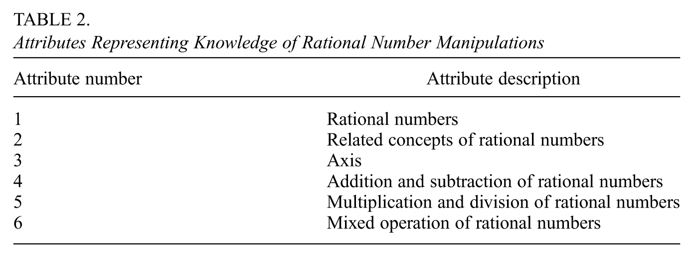
We apply the model to the dataset (Zhan, 2021) used in Tang and Zhan (2021), a study that aimed to measure the effectiveness of two types of feedback for math test takers: CDF (cognitive diagnostic feedback) and CIRF (correct-incorrect response feedback). The test had 18 items, 12 of which were multiple-choice and 6 of which were calculations. The items were designed to diagnose whether or not students had mastered six latent attributes related to rational number operations (Tang & Zhan, 2020). The six latent binary attributes are displayed in Table 2. We note that in their study, Tang and Zhan (2021) designed a $Q$ -matrix which reflects their assumptions of which latent attributes (representing mathematics skills) would need to be mastered in order to score correctly on each of the items. As noted in the Introduction, the particular definition of the $Q$ -matrix depends on the model being specified. In the case of Tang and Zhan (2021), their sLong-DINA model has no interaction terms, so a 1 for a particular attribute-item pair in the $Q$ -matrix indicates that the attribute can enter into the equation for the latent state-conditional response probability for that item.

Table 2.

Attributes Representing Knowledge of Rational Number Manipulations

Attribute number	Attribute description
1	Rational numbers
2	Related concepts of rational numbers
3	Axis
4	Addition and subtraction of rational numbers
5	Multiplication and division of rational numbers
6	Mixed operation of rational numbers

The dataset consists of item response data for 276 respondents. The respondents are grouped into almost equal-sized groupings: the diagnosis group, the traditional group, and the control group. Respondents took a math test three times, and thus the item response data consists of binary values indicating a correct or incorrect answer for each of the 18 items observed at three time points. The protocol was as follows: all respondents took the test once, and 24 hours afterwards, CDF was provided to the diagnosis group and CIRF was provided to the traditional group. The control group received no feedback. One week after the first test, the respondents took the test a second time, and feedback was once again provided to the different groups as above. Finally, all respondents took the test a third time after 1 week had passed.

We fit our longitudinal model, which is exploratory, to this dataset for values of $K$ ranging from 2 through 6, with a measurement model order of 2 (i.e., including one-way main effects and two-way interactions) for interpretability. We also fit a confirmatory version of our model, which uses a fixed $δ$ matrix corresponding to the fixed $Q$ -matrix of Tang and Zhan (2021) rather than estimating $δ$ from the data. Dummy variables indicating the three groupings of respondents were used as covariates. We set hyperparameter values to $σ_{β}^{2} = 2.0$ , $ω_{0} = 0.5$ , and $ω_{1} = 0.5$ , $a = 1, 000^{- 1}$ , and $v_{0} = K + 1$ . We performed hyperparameter tuning on $σ_{κ}^{2}$ and chose its value such that its acceptance rate is roughly 40%. We specify the order of the transition model to be 1 (only main effects). We ran the model using a burn-in period of 10,000 draws and a post-burn-in period of 20,000 draws. We consider two diagnostics for convergence, the Geweke test and the IAT. We observe that fewer than 2% of the Geweke test statistics fall outside the 95% confidence interval, and that, on average, for each parameter, the effective sample size (number of draws divided by IAT) is greater than 200.

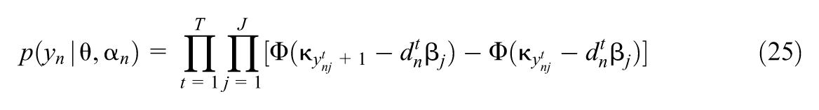
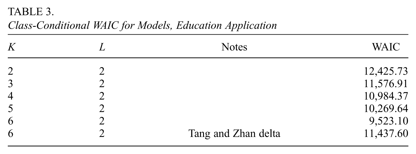
We utilize the Widely Applicable Information Criterion, or WAIC (Watanabe, 2010) to evaluate the choice of model (i.e. the choice of various possible values of $K$ and $L$ ). The WAIC is an estimate of the generalization loss of a Bayesian model; the smaller is generalization loss, the smaller is the Kullback-Leibler distance from the true distribution to the posterior predictive distribution obtained from the selected model and the observed data. Here we use class-conditional values of the likelihood to calculate the WAIC (Merkle et al., 2019). We store values of the conditional likelihood

p (y_{n} ∣ θ, α_{n}) = \prod_{t = 1}^{T} \prod_{j = 1}^{J} [Φ (κ_{y_{n j}^{t} + 1} - d_{n}^{t} β_{j}) - Φ (κ_{y_{n j}^{t}} - d_{n}^{t} β_{j})]

(25)

evaluated at each $(θ^{(s)}, α^{(s)})$ in the post-burn-in phase of our sampling, using a thinning interval of 10 (see Supplemental Material I [available in the online version of this article] for derivation). These values were evaluated using the waic function of the R package loo (Vehtari et al., 2024). The resulting WAIC values are displayed in Table 3.

Table 3.

Class-Conditional WAIC for Models, Education Application

$K$	$L$	Notes	WAIC
2	2		12,425.73
3	2		11,576.91
4	2		10,984.37
5	2		10,269.64
6	2		9,523.10
6	2	Tang and Zhan delta	11,437.60

We observe that our model, with its exploratory $δ$ matrix, has a better fit than the model of Tang and Zhan (2021) for all values of $K$ greater than 3. We consider the parameter estimates for the $K = 6$ case since Tang and Zhan (2021) assumed six attributes for their model and $K = 6$ had the lowest WAIC value, indicating the best fit. The run time for this model with the above chain length was 12.194 minutes, utilizing 4 cores of an 11th Gen Intel(R) Core(TM) i7-1160G7 processor on a machine with 16 GB of RAM.

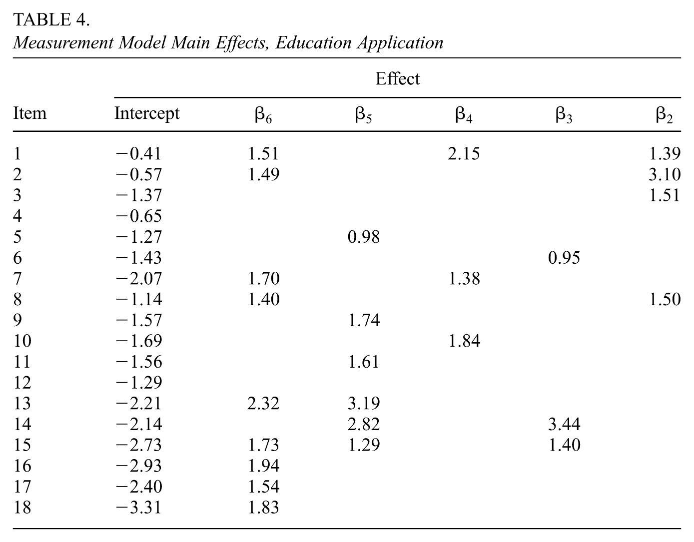
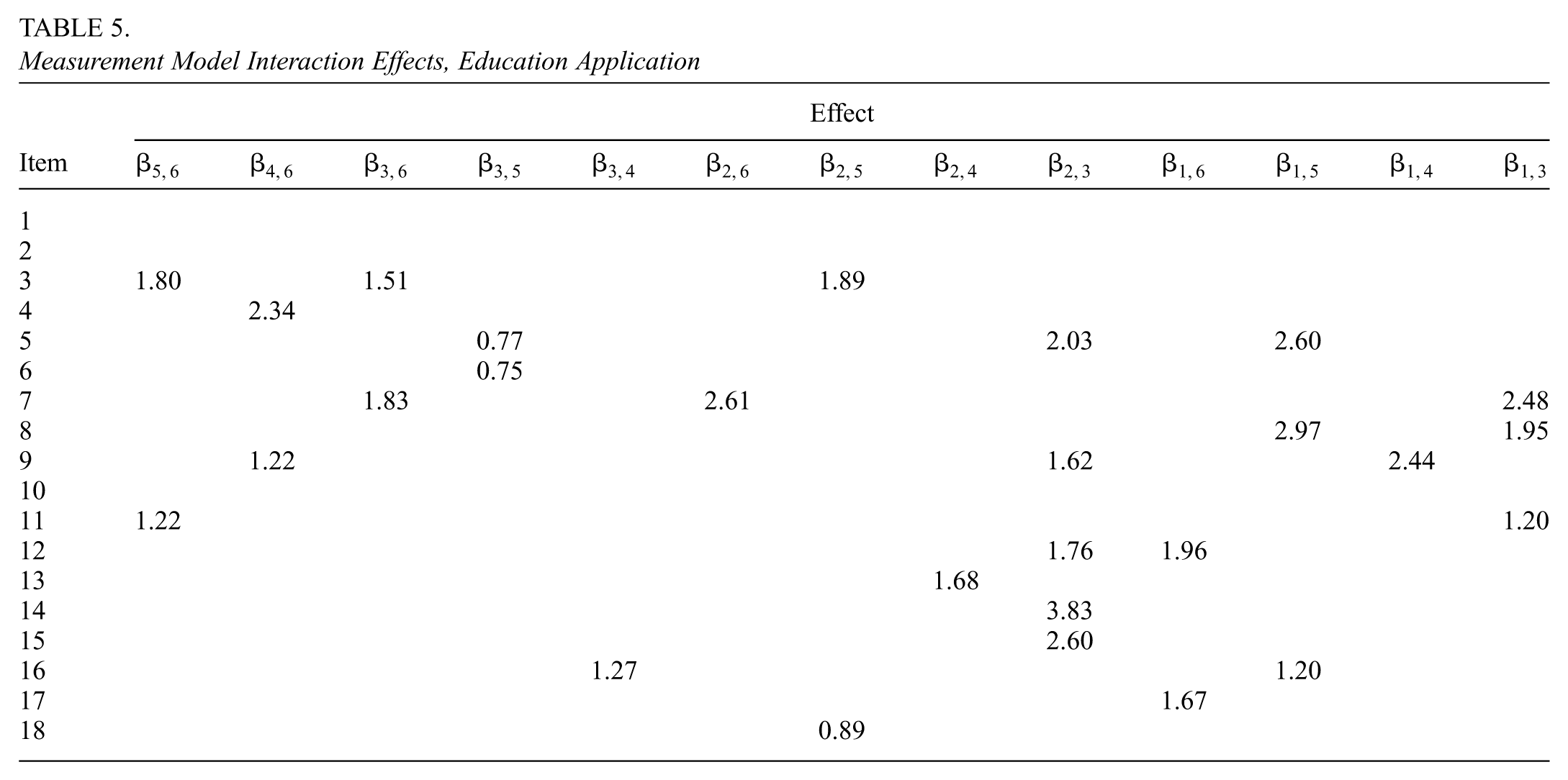
The estimate of the $β$ matrix (the average of draws of $β$ ) is shown in Table 4 (which shows the main effects) and Table 5 (which shows the interaction effects). $β_{k}$ indicates the main effects for attribute $k$ , and $β_{k, l}$ indicates the effects of the interaction of attributes $k$ and $l$ . We have applied a sparsity criterion, namely that any element of $β$ for which 0 falls into the 95% equal-tail credible interval is deemed inactive. Attributes which had no significant effects were excluded from the tables. Attribute 1 has no significant main effects, and all other attributes load onto a different combination of items. Items 4 and 12 correspond to no main effects. Interaction effects are present for all items other than 1, 2, and 10. We observe a significant amount of sparsity for main effects, where most pairs of attributes are related to one, two, or three items through interaction effects (one pair of attributes, attributes 1 and 6, have an interaction effect which loads on five items).

Table 4.

Measurement Model Main Effects, Education Application

	Effect
Item	Intercept	$β_{6}$	$β_{5}$	$β_{4}$	$β_{3}$	$β_{2}$
1	−0.41	1.51		2.15		1.39
2	−0.57	1.49				3.10
3	−1.37					1.51
4	−0.65
5	−1.27		0.98
6	−1.43				0.95
7	−2.07	1.70		1.38
8	−1.14	1.40				1.50
9	−1.57		1.74
10	−1.69			1.84
11	−1.56		1.61
12	−1.29
13	−2.21	2.32	3.19
14	−2.14		2.82		3.44
15	−2.73	1.73	1.29		1.40
16	−2.93	1.94
17	−2.40	1.54
18	−3.31	1.83

Table 5.

Measurement Model Interaction Effects, Education Application

	Effect
Item	$β_{5, 6}$	$β_{4, 6}$	$β_{3, 6}$	$β_{3, 5}$	$β_{3, 4}$	$β_{2, 6}$	$β_{2, 5}$	$β_{2, 4}$	$β_{2, 3}$	$β_{1, 6}$	$β_{1, 5}$	$β_{1, 4}$	$β_{1, 3}$
1
2
3	1.80		1.51				1.89
4		2.34
5				0.77					2.03		2.60
6				0.75
7			1.83			2.61							2.48
8											2.97		1.95
9		1.22							1.62			2.44
10
11	1.22												1.20
12									1.76	1.96
13								1.68
14									3.83
15									2.60
16					1.27						1.20
17										1.67
18							0.89

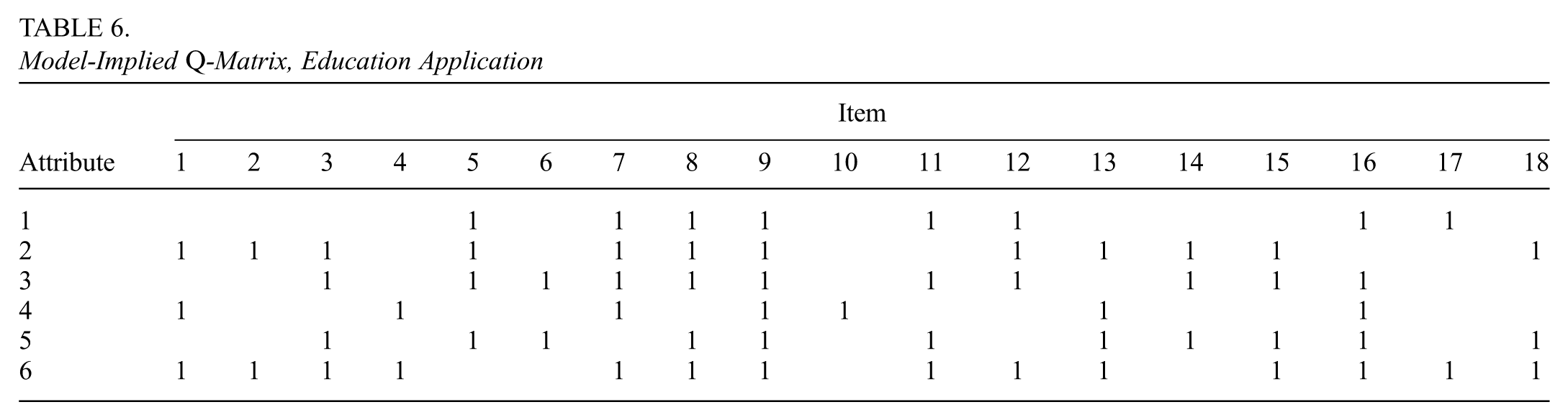
We examine the $Q$ -matrix implied by the significant measurement model coefficients, which is shown in Table 6. This $Q$ -matrix is significantly denser than the one hypothesized by Tang and Zhan: it shows many items being related to at least three attributes and some related to more, with only one item being related to a single attribute.

Table 6.

Model-Implied $Q$ -Matrix, Education Application

	Item
Attribute	1	2	3	4	5	6	7	8	9	10	11	12	13	14	15	16	17	18
1					1		1	1	1		1	1				1	1
2	1	1	1		1		1	1	1			1	1	1	1			1
3			1		1	1	1	1	1		1	1		1	1	1
4	1			1			1		1	1			1			1
5			1		1	1		1	1		1		1	1	1	1		1
6	1	1	1	1			1	1	1		1	1	1		1	1	1	1

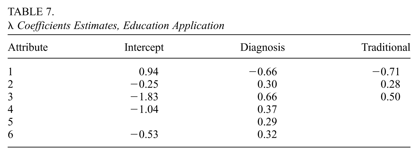
The estimates of the slope coefficient relating the latent state to covariates, $λ$ , are shown in Table 7. We see that the diagnosis intervention (CDF) has a positive effect on every attribute except attribute 1, for which the effect was negative. We see that the traditional intervention (CIRF) has positive effects on attributes 2 and 3 and a negative effect on attribute 1 (attributes 4 through 6 were not significant). These results correspond to the conclusions of Tang and Zhan (2021), which are that CDF is more effective than no feedback, and CDF is more effective than CIRF. For the 95% equal-tail credible intervals for each coefficient of $λ$ , see Supplemental Material J (available in the online version of this article).

Table 7.

$λ$ Coefficients Estimates, Education Application

Attribute	Intercept	Diagnosis	Traditional
1	0.94	−0.66	−0.71
2	−0.25	0.30	0.28
3	−1.83	0.66	0.50
4	−1.04	0.37
5		0.29
6	−0.53	0.32

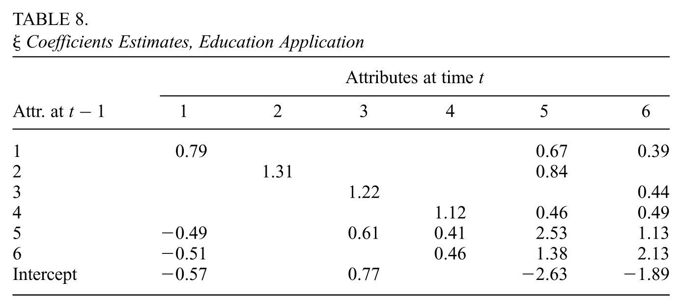
The matrix of coefficients $ξ$ indicates how a respondent’s attributes at a time point are affected by the respondent’s attributes at the previous time point. The estimate of $ξ$ is shown in Table 8. We see that there is a large positive number for each entry of the main diagonal of the table, which shows that if attribute $k$ is present at time $t - 1$ , it is likely to be present at $t$ as well (in the context of this application, this means that skills once mastered are maintained across time). Most relationships between attributes between sequential time points are positive. For the 95% equal-tail credible intervals for each coefficient of $ξ$ , see Supplemental Material J (available in the online version of this article).

Table 8.

$ξ$ Coefficients Estimates, Education Application

	Attributes at time $t$
Attr. at $t - 1$	1	2	3	4	5	6
1	0.79				0.67	0.39
2		1.31			0.84
3			1.22			0.44
4				1.12	0.46	0.49
5	−0.49		0.61	0.41	2.53	1.13
6	−0.51			0.46	1.38	2.13
Intercept	−0.57		0.77		−2.63	−1.89

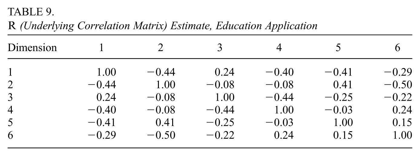
Table 9 shows the estimates of the underlying correlation matrix relating the six attributes of the latent state. We observe almost no correlation between attribute pairs (2, 3), (2, 4), and (4, 5). We observe several correlations close to negative and positive 0.5.

Table 9.

$R$ (Underlying Correlation Matrix) Estimate, Education Application

Dimension	1	2	3	4	5	6
1	1.00	−0.44	0.24	−0.40	−0.41	−0.29
2	−0.44	1.00	−0.08	−0.08	0.41	−0.50
3	0.24	−0.08	1.00	−0.44	−0.25	−0.22
4	−0.40	−0.08	−0.44	1.00	−0.03	0.24
5	−0.41	0.41	−0.25	−0.03	1.00	0.15
6	−0.29	−0.50	−0.22	0.24	0.15	1.00

8.2 Emotional State Application

We apply the model to response data (Shui et al., 2020) collected from 140 respondents over a period of 5 days (Shui et al., 2021) (two respondents from the original dataset with entire days of data missing were excluded). Data were collected by a device distributed to all participants which sent a request to the participant at six varying time points per day with a minimal interval of 90 minutes between requests (Shui et al., 2021). The response data was missing some time points for some respondents; we assume that these data points were missing completely at random (Little, 2021; Marini et al., 1980). The missing data vectors are treated as a parameter with the same conditional independence and dependence assumptions in the graphical model as $Y$ . We sample from the augmented posterior: the sampling algorithm remains the same with one additional step of sampling the various $Y_{n}^{t}$ as follows. For each respondent $n$ , the known vector of time points for which $Y_{n}^{t}$ is missing is denoted $(t_{n}^{1}, \dots, t_{n}^{i})$ , $i \in [T]$ . For respondent $n$ , for each time point $t \in (t_{n}^{1}, \dots, t_{n}^{i})$ of missing data, the conditional of $Y_{nj}^{t}$ collapsed on $Y_{nj}^{*, t}$ is a categorical distribution with

p (Y_{nj}^{t} = m ∣ α_{n}^{t}, β_{j}, κ_{j}) = Φ (κ_{j, m + 1} - d_{n}^{t} β_{j}) - Φ (κ_{j, m} - d_{n}^{t} β_{j}) .

(26)

Details on how time points for missingness and data initialization were handled are in Supplemental Material K (available in the online version of this article).

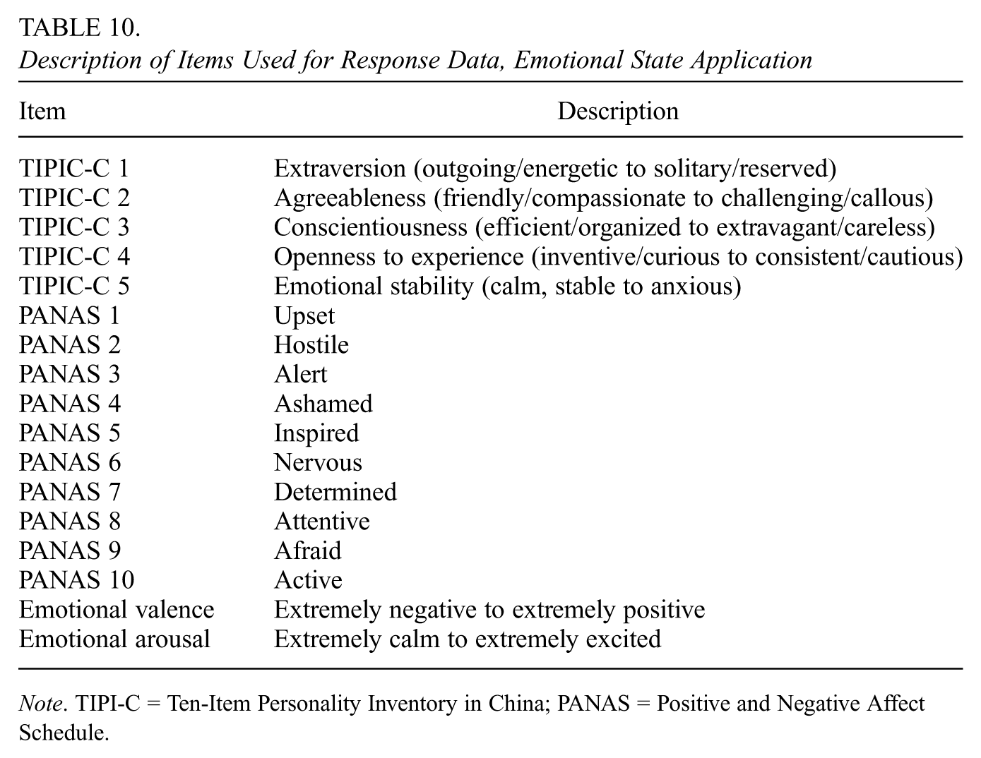
The response data consisted of 17 items, listed in the Item column of Table 10: five items described as the Ten-Item Personality Inventory in China (TIPI-C; Lu et al., 2020; Shui et al., 2020, 2021), the ten-item Positive and Negative Affect Schedule (PANAS; Watson et al., 1988), emotional valence, and emotional arousal. The TIPIC-C items range from 0 through 6, the PANAS items range from 0 through 4, and the valence and arousal items range from 0 through 4.

Table 10.

Description of Items Used for Response Data, Emotional State Application

Item	Description
TIPIC-C 1	Extraversion (outgoing/energetic to solitary/reserved)
TIPIC-C 2	Agreeableness (friendly/compassionate to challenging/callous)
TIPIC-C 3	Conscientiousness (efficient/organized to extravagant/careless)
TIPIC-C 4	Openness to experience (inventive/curious to consistent/cautious)
TIPIC-C 5	Emotional stability (calm, stable to anxious)
PANAS 1	Upset
PANAS 2	Hostile
PANAS 3	Alert
PANAS 4	Ashamed
PANAS 5	Inspired
PANAS 6	Nervous
PANAS 7	Determined
PANAS 8	Attentive
PANAS 9	Afraid
PANAS 10	Active
Emotional valence	Extremely negative to extremely positive
Emotional arousal	Extremely calm to extremely excited

Note. TIPI-C = Ten-Item Personality Inventory in China; PANAS = Positive and Negative Affect Schedule.

We used four covariates for the analysis. The first two were dummy variables indicating time range of measurement, namely afternoon (12:30–18:29) and evening (18:30–23:59) as opposed to a baseline of morning (07:00–12:29). The other two are from the pre-test measurements, specifically from the Meaning of Life Questionnaire (MLQ; Steger et al., 2006): we computed the two subscales for presence and search and use the $z$ -scores of these as our other two covariates.

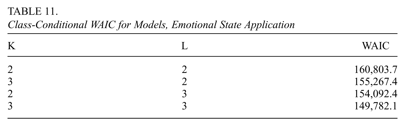
We fit five different models of increasing complexity, four of which are displayed in Table 11 along with class-conditional WAIC values calculated as they were in the education application. For one of the five models, $K = 4, L = 2$ , we observed near collinearity between two latent attributes so we excluded this model from our consideration, and took this as evidence that the latent space has under four dimensions. We selected the model with the lowest WAIC value, namely $K = 3, L = 3$ . The chains had a burn-in period of 20,000 draws and a post-burn-in phase of 20,000 draws. The run time for this model and chain length was 47.880 minutes, utilizing 4 cores of an 11th Gen Intel(R) Core(TM) i7-1160G7 processor on a machine with 16 GB of RAM. As in the previous application, we use both the Geweke test and the IAT to evaluate convergence. The Geweke test statistic for every single one of the parameters falls within the 95% acceptance region; on average for each parameter the effective sample size is always greater than 100.

Table 11.

Class-Conditional WAIC for Models, Emotional State Application

K	L	WAIC
2	2	160,803.7
3	2	155,267.4
2	3	154,092.4
3	3	149,782.1

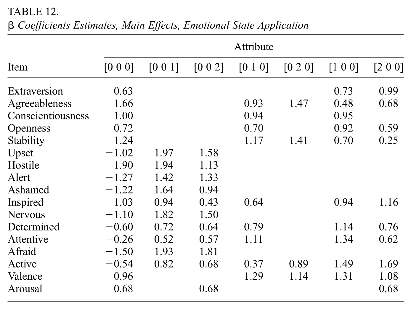
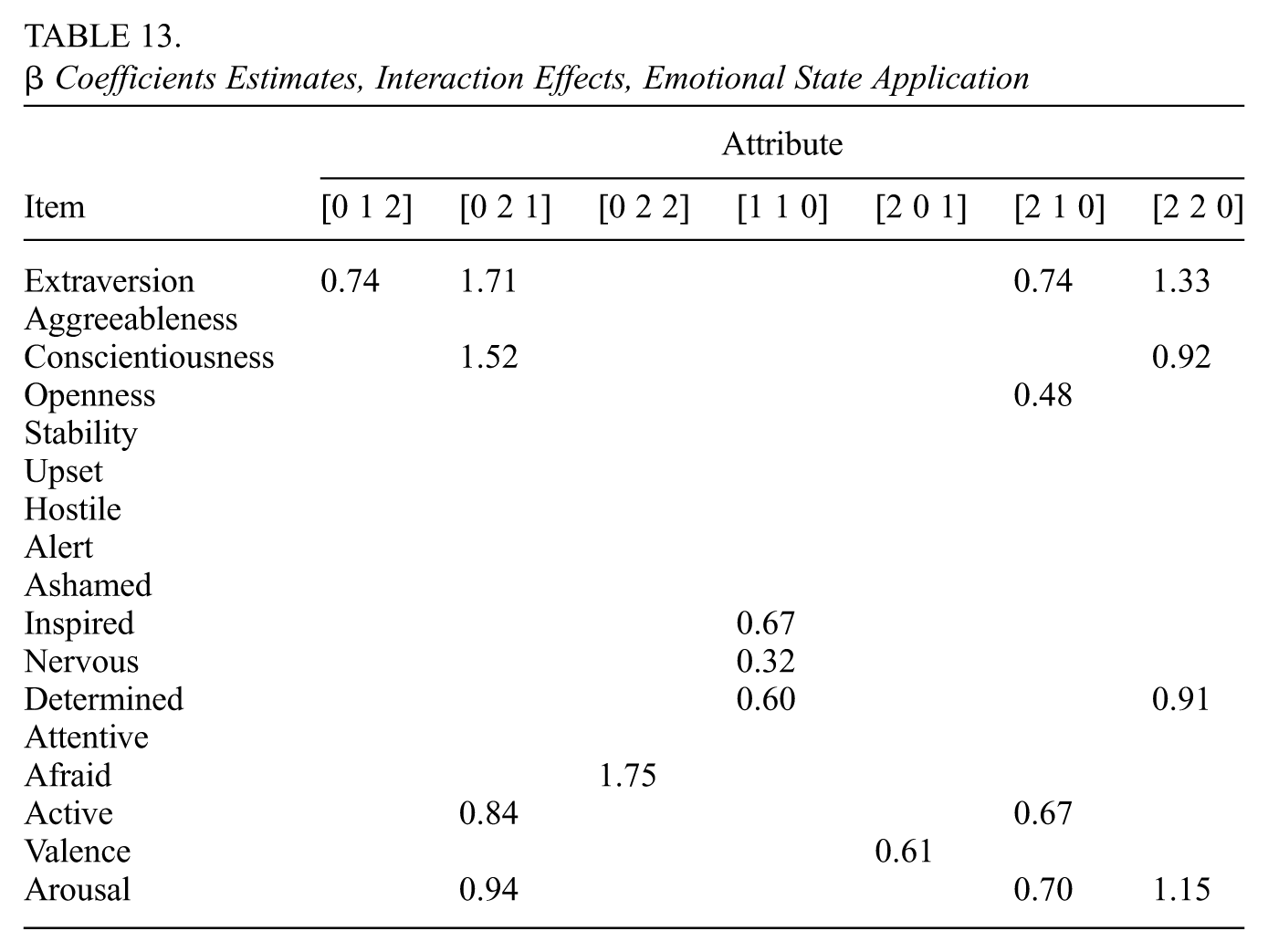
Tables 12 and 13 display the model’s estimates of $β$ . We see in Table 12 that some groups of items are related to only one dimension of the latent state: the TIPIC-C (personality) items are related to attributes 1 and 2 only, while the seven of the ten PANAS (affect) items are only related to attribute 3. In Table 13, we see that six of the items are involved in no interaction effects. For most of the items for which there are interaction effects, taking into account the attributes involved in both the main and interaction effects leads us to conclude that such items are involved in some way with all three attributes. Supplemental Material K (available in the online version of this article) contains further details of the data analysis.

Table 12.

$β$ Coefficients Estimates, Main Effects, Emotional State Application

	Attribute
Item	[0 0 0]	[0 0 1]	[0 0 2]	[0 1 0]	[0 2 0]	[1 0 0]	[2 0 0]
Extraversion	0.63					0.73	0.99
Agreeableness	1.66			0.93	1.47	0.48	0.68
Conscientiousness	1.00			0.94		0.95
Openness	0.72			0.70		0.92	0.59
Stability	1.24			1.17	1.41	0.70	0.25
Upset	−1.02	1.97	1.58
Hostile	−1.90	1.94	1.13
Alert	−1.27	1.42	1.33
Ashamed	−1.22	1.64	0.94
Inspired	−1.03	0.94	0.43	0.64		0.94	1.16
Nervous	−1.10	1.82	1.50
Determined	−0.60	0.72	0.64	0.79		1.14	0.76
Attentive	−0.26	0.52	0.57	1.11		1.34	0.62
Afraid	−1.50	1.93	1.81
Active	−0.54	0.82	0.68	0.37	0.89	1.49	1.69
Valence	0.96			1.29	1.14	1.31	1.08
Arousal	0.68		0.68				0.68

Table 13.

$β$ Coefficients Estimates, Interaction Effects, Emotional State Application

	Attribute
Item	[0 1 2]	[0 2 1]	[0 2 2]	[1 1 0]	[2 0 1]	[2 1 0]	[2 2 0]
Extraversion	0.74	1.71				0.74	1.33
Aggreeableness
Conscientiousness		1.52					0.92
Openness						0.48
Stability
Upset
Hostile
Alert
Ashamed
Inspired				0.67
Nervous				0.32
Determined				0.60			0.91
Attentive
Afraid			1.75
Active		0.84				0.67
Valence					0.61
Arousal		0.94				0.70	1.15

9 Discussion

In this paper, we introduced a longitudinal extension of a cross-sectional RLCM with polytomous attributes and covariates. The model has similarities to a previous model introduced by Bartolucci et al. (2012) but provides a new structure, namely a multivariate probit specification for the transition model, which incorporates covariates through the mean of the continuous random vector underlying the discrete latent state vector. The modeling technique presented here lends itself more to diagnosis than do latent trait models such as item response theory or factor analysis. In educational studies, it is often of interest to see how skill mastery can change over time, in particular for measuring the effects of interventions. Here, a Markov modeling approach was presented with covariates with quantifiable effects on transitioning among the latent states. A flexible feature of this model is that the relationship between the item response probabilities and the latent state need not be specified explicitly beforehand, and can be discovered accurately through an exploratory Bayesian approach. In fact, the results from our education application provide evidence that our exploratory model provided improved fit to an educational intervention study in comparison to a confirmatory RLCM as described in previous research. One implication is that our methods can be used to validate expert knowledge about the underlying $Q$ -matrix and provide a more precise framework for evaluating intervention effects.

A Bayesian modeling approach and corresponding estimation algorithm were presented and shown through simulation to perform well under a variety of settings. In addition to being able to recover the underlying latent structure, our parameter expansion algorithm provides an efficient approach for inferring the parameters of the multivariate probit. Specifically, sampling the multivariate probit correlation matrix and thresholds is notoriously difficult. Our simulation results provide evidence that our novel Bayesian formulation was effective in the thresholds and attribute correlations.

As demonstrated in the emotional state application, we have extended the algorithm to handle intermittent missing data by treating the unobserved responses like other parameters of the model. This is a more efficient alternative to multiple imputation techniques that are common in the literature and gives a simple approach to addressing missing data, which is always an issue in studies such as the one we have presented. One avenue for future work would be to apply the model in a mental health or medical setting where patients transition between states: the model would help researchers evaluate the impact of cognitive therapies or medical treatments.

Supplemental Material

sj-pdf-1-jeb-10.3102_10769986251415569 – Supplemental material for A Restricted Latent Class Hidden Markov Model for Polytomous Responses, Polytomous Attributes, and Covariates: Identifiability and Application

Supplemental material, sj-pdf-1-jeb-10.3102_10769986251415569 for A Restricted Latent Class Hidden Markov Model for Polytomous Responses, Polytomous Attributes, and Covariates: Identifiability and Application by Eric Alan Wayman, Steven Andrew Culpepper, Jeff Douglas and Jesse Bowers in Journal of Educational and Behavioral Statistics

Footnotes

Declaration of Conflicting Interests

The authors declared no potential conflicts of interest with respect to the research, authorship, and/or publication of this article.

Funding

The authors disclosed receipt of the following financial support for the research, authorship, and/or publication of this article: This work was partially supported by the U.S. National Science Foundation, under award numbers SES 2150628 and SES 1951057.

ORCID iDs

Eric Alan Wayman

Steven Andrew Culpepper

Data Availability Statement

The data (Zhan, 2021) analyzed in the education application are available in the openICPSR repository, https://doi.org/10.3886/E153061V1. The data (Shui et al., 2020) analyzed in the emotional state application are available in the Synapse repository, .

Authors

ERIC ALAN WAYMAN is a PhD student in the Department of Statistics at the University of Illinois Urbana- Champaign, Computing Applications Building, Room 156, 605 E. Springfield Ave., Champaign, IL 61820; email: ericwaymanpublications@mailworks.org. His research interests include Bayesian models and computation, restricted latent class models, and longitudinal modeling.

STEVEN ANDREW CULPEPPER is a professor in the Department of Statistics at the University of Illinois Urbana-Champaign, Computing Applications Building, Room 156, 605 E. Springfield Ave., Champaign, IL 61820; email: sculpepp@illinois.edu. His research interests include large-scale testing, Bayesian models and computation, restricted latent class models, and longitudinal modeling.

JEFF DOUGLAS is a professor in the Department of Statistics at the University of Illinois Urbana-Champaign, Computing Applications Building, Room 156, 605 E. Springfield Ave., Champaign, IL 61820; email: jeff-doug@illinois.edu. His research interests include multivariate latent variable methodology for educational and psychological testing with an emphasis on cognitive diagnosis and item response theory.

JESSE BOWERS is a PhD student in the Department of Statistics at the University of Illinois Urbana-Champaign, Computing Applications Building, Room 156, 605 E. Springfield Ave., Champaign, IL 61820; e-mail: bowers.jesse+publications@gmail.com. His research interests include Bayesian latent variable models.

References

Agresti

(2015). Foundations of linear and generalized linear models. Wiley.

Ashford

J. R.

Sowden

R. R.

(1970). Multi-variate probit analysis. Biometrics, 26(3), 535–546. https://doi.org/10.2307/2529107

Barnard

McCulloch

Meng

X.-L.

(2000). Modeling covariance matrices in terms of standard deviations and correlations, with application to shrinkage. Statistica Sinica, 10(4), 1281–1311. https://www3.stat.sinica.edu.tw/statistica/oldpdf/A10n416.pdf

Bartolucci

Farcomeni

(2009). A multivariate extension of the dynamic logit model for longitudinal data based on a latent Markov heterogeneity structure. Journal of the American Statistical Association, 104(486), 816–831. https://doi.org/10.1198/jasa.2009.0107

Bartolucci

Farcomeni

Pennoni

(2012). Latent Markov models for longitudinal data. CRC Press. https://doi.org/10.1201/b13246

Baum

L. E.

Petrie

(1966). Statistical inference for probabilistic functions of finite state Markov chains. The Annals of Mathematical Statistics, 37(6), 1554–1563. https://doi.org/10.1214/aoms/1177699147

Chen

de la Torre

(2013). A general cognitive diagnosis model for expert-defined polytomous attributes. Applied Psychological Measurement, 37(6), 419–437. https://doi.org/10.1177/0146621613479818

Chen

Culpepper

S. A.

(2020). A multivariate probit model for learning trajectories: A fine-grained evaluation of an educational intervention. Applied Psychological Measurement, 44(7–8), 515–530. https://doi.org/10.1177/0146621620920928

Chen

Culpepper

S. A.

Wang

Douglas

(2018). A hidden Markov model for learning trajectories in cognitive diagnosis with application to spatial rotation skills. Applied Psychological Measurement, 42(1), 5–23. https://doi.org/10.1177/0146621617721250

10.

Chen

Culpepper

Liang

(2020). A sparse latent class model for cognitive diagnosis. Psychometrika, 85(1), 121–153. https://doi.org/10.1007/s11336-019-09693-2

11.

Chib

(2011). Introduction to simulation and MCMC methods. In Geweke

Koop

Van Dijk

(Eds.), The Oxford handbook of Bayesian econometrics (pp. 183–217). Oxford University Press. https://doi.org/10.1093/oxfordhb/9780199559084.013.0006

12.

Christoffersson

(1975). Factor analysis of dichotomized variables. Psychometrika, 40(1), 5–32. https://doi.org/10.1007/BF02291477

13.

Collins

L. M.

Wugalter

S. E.

(1992). Latent class models for stage-sequential dynamic latent variables. Multivariate Behavioral Research, 27(1), 131–157. https://doi.org/10.1207/s15327906mbr2701_8

14.

Culpepper

S. A.

(2019). An exploratory diagnostic model for ordinal responses with binary attributes: Identifiability and estimation. Psychometrika, 84(4), 921–940. https://doi.org/10.1007/s11336-019-09683-4

15.

Gelman

Hill

(2007). Data analysis using regression and multilevel/hierarchical models. Cambridge University Press. https://doi.org/10.1017/CBO9780511790942

16.

Geweke

(1992). Evaluating the accuracy of sampling-based approaches to the calculation of posterior moments. In Bernardo

J.-M.

Berger

J. O.

Dawid

A. P.

Smith

A. F. M.

(Eds.), Bayesian statistics 4: Proceedings of the Fourth Valencia International Meeting, dedicated to the memory of Morris H. DeGroot, 1931–1989 (pp. 169–193). Oxford University Press. https://doi.org/10.1093/oso/9780198522669.003.0010

17.

Goodman

L. A.

(1974). Exploratory latent structure analysis using both identifiable and unidentifiable models. Biometrika, 61(2), 215–231. https://doi.org/10.1093/biomet/61.2.215

18.

Haertel

(1984). An application of latent class models to assessment data. Applied Psychological Measurement, 8(3), 333–346. https://doi.org/10.1177/014662168400800311

19.

Haertel

E. H.

(1990). Continuous and discrete latent structure models for item response data. Psychometrika, 55(3), 477–494. https://doi.org/10.1007/BF02294762

20.

Hagenaars

J. A.

(1990). Categorical longitudinal data: Log-linear panel, trend, and cohort analysis. SAGE Publications.

21.

Culpepper

S. A.

Douglas

(2023). A sparse latent class model for polytomous attributes in cognitive diagnostic assessments. In van der Ark

L. A.

Emons

W. H. M.

Meijer

R. R.

(Eds.), Essays on contemporary psychometrics (pp. 413–442). Springer International Publishing. https://doi.org/10.1007/978-3-031-10370-4_21

22.

Kaya

Leite

W. L.

(2017). Assessing change in latent skills across time with longitudinal cognitive diagnosis modeling: An evaluation of model performance. Educational and Psychological Measurement, 77(3), 369–388. https://doi.org/10.1177/0013164416659314

23.

Kuo

Mallick

(1998). Variable selection for regression models. Sankhyā: The Indian Journal of Statistics, Series B, 60(1), 65–81.

24.

Lauritzen

S. L.

(1996). Graphical models. Clarendon Press. https://doi.org/10.1093/oso/9780198522195.001.0001

25.

Cohen

Bottge

Templin

(2016). A latent transition analysis model for assessing change in cognitive skills. Educational and Psychological Measurement, 76(2), 181–204. https://doi.org/10.1177/0013164415588946

26.

Little

R. J.

(2021). Missing data assumptions. Annual Review of Statistics and its Application, 8, 89–107. https://doi.org/10.1146/annurev-statistics-040720-031104

27.

Liu

(2008). Monte Carlo strategies in scientific computing. Springer Science+Business Media New York. https://doi.org/10.1007/978-0-387-76371-2

28.

Liu

J. S.

Y. N.

(1999). Parameter expansion for data augmentation. Journal of the American Statistical Association, 94(448), 1264–1274. https://doi.org/10.2307/2669940

29.

Liu

Ying

(2013). Theory of self-learning Q-matrix. Bernoulli, 19(5A), 1790–1817. https://doi.org/10.3150/12-BEJ430

30.

Liu

Culpepper

S. A.

Chen

(2023). Identifiability of hidden Markov models for learning trajectories in cognitive diagnosis. Psychometrika, 88(2), 361–386. https://doi.org/10.1007/s11336-023-09904-x

31.

J. G.

Liu

X. L.

Liao

Wang

(2020). Disentangling stereotypes from social reality: Astrological stereotypes and discrimination in China. Journal of Personality and Social Psychology, 119(6), 1359–1379. https://doi.org/10.1037/pspi0000237

32.

Madison

M. J.

Bradshaw

L. P.

(2018). Assessing growth in a diagnostic classification model framework. Psychometrika, 83(4), 963–990. https://doi.org/10.1007/s11336-018-9638-5

33.

Madison

M. J.

Jeon

Cotterell

Haab

Zor

(2025). TDCM: An R package for estimating longitudinal diagnostic classification models. Multivariate Behavioral Research, 60(3), 518–527. https://doi.org/10.1080/00273171.2025.2453454

34.

Marini

M. M.

Olsen

A. R.

Rubin

D. B.

(1980). Maximum-likelihood estimation in panel studies with missing data. Sociological Methodology, 11, 314–357. https://doi.org/10.2307/270868

35.

McDonald

R. P.

(1967). Nonlinear factor analysis. Psychometric Society.

36.

McGibbon

R. T.

(2015). pyhmc: Hamiltonian Monte Carlo in Python [Computer software]. https://github.com/rmcgibbo/pyhmc

37.

Meng

X.-L.

Van Dyk

D. A.

(1999). Seeking efficient data augmentation schemes via conditional and marginal augmentation. Biometrika, 86(2), 301–320. https://doi.org/10.1093/biomet/86.2.301

38.

Merkle

E. C.

Furr

Rabe-Hesketh

(2019). Bayesian comparison of latent variable models: Conditional versus marginal likelihoods. Psychometrika, 84(3), 802–829. https://doi.org/10.1007/s11336-019-09679-0

39.

Miller

J. W.

(2016). Hidden Markov models [Lecture notes]. https://jwmi.github.io/ASM/5-HMMs.pdf

40.

Murphy

K. P.

(2012). Machine learning: A probabilistic perspective. MIT Press.

41.

Muthén

(1978). Contributions to factor analysis of dichotomous variables. Psychometrika, 43(4), 551–560. https://doi.org/10.1007/BF02293813

42.

Plummer

Best

Cowles

Vines

(2006). CODA: Convergence diagnosis and output analysis for MCMC. R News, 6(1), 7–11. https://journal.r-project.org/articles/RN-2006-002/RN-2006-002.pdf

43.

Poulsen

C. S.

(1983). Latent structure analysis with choice modeling applications (Publication No. 1983.8316074) [Doctoral dissertation, University of Pennsylvania]. ProQuest Dissertations & Theses Global.

44.

Rupp

A. A.

Templin

Henson

R. A.

(2010). Diagnostic measurement: Theory, methods, and applications. The Guilford Press.

45.

Sanderson

Curtin

(2019). Practical sparse matrices in C++ with hybrid storage and template-based expression optimisation. Mathematical and Computational Applications, 24(3), Article 70. https://doi.org/10.3390/mca24030070

46.

Sanderson

Curtin

(2025). Armadillo: An efficient framework for numerical linear algebra. In 2025 17th International Conference on Computer and Automation Engineering (ICCAE) (pp. 303–307). https://doi.org/10.1109/ICCAE64891.2025.10980539

47.

Seneta

(2006). Non-negative matrices and Markov chains. Springer Science+Business Media. https://doi.org/10.1007/0-387-32792-4

48.

Shui

Zhang

Wang

Zhang

(2020). DAPPER dataset [Data set]. Synapse. https://doi.org/10.7303/syn22418021

49.

Shui

Zhang

Wang

Zhang

(2021). A dataset of daily ambulatory psychological and physiological recording for emotion research. Scientific Data, 8, Article 161. https://doi.org/10.1038/s41597-021-00945-4

50.

Steger

M. F.

Frazier

Oishi

Kaler

(2006). The Meaning in Life Questionnaire: Assessing the presence of and search for meaning in life. Journal of Counseling Psychology, 53(1), 80–93. https://doi.org/10.1037/0022-0167.53.1.80

51.

Sun

Xin

Zhang

de la Torre

(2013). A polytomous extension of the generalized distance discriminating method. Applied Psychological Measurement, 37(7), 503–521. https://doi.org/10.1177/0146621613487254

52.

Tang

Zhan

(2020). The development of an instrument for longitudinal learning diagnosis of rational number operations based on parallel tests. Frontiers in Psychology, 11, Article 2246. https://doi.org/10.3389/fpsyg.2020.02246

53.

Tang

Zhan

(2021). Does diagnostic feedback promote learning? Evidence from a longitudinal cognitive diagnostic assessment. AERA Open, 7(1), 1–15. https://doi.org/10.1177/23328584211060804

54.

van de Pol

Langeheine

(1990). Mixed Markov latent class models. Sociological Methodology, 20, 213–247. https://doi.org/10.2307/271087

55.

Vehtari

Gabry

Magnusson

Yao

Bürkner

P.-C.

Paananen

Gelman

(2024). loo: Efficient leave-one-out cross-validation and WAIC for Bayesian models [Computer software]. https://mc-stan.org/loo/

56.

Vermunt

J. K.

(2001). The use of restricted latent class models for defining and testing nonparametric and parametric item response theory models. Applied Psychological Measurement, 25(3), 283–294. https://doi.org/10.1177/01466210122032082

57.

Wang

Yang

Culpepper

S. A.

Douglas

J. A.

(2018). Tracking skill acquisition with cognitive diagnosis models: A higher-order, hidden Markov model with covariates. Journal of Educational and Behavioral Statistics, 43(1), 57–87. https://doi.org/10.3102/1076998617719727

58.

Watanabe

(2010). Asymptotic equivalence of Bayes cross validation and widely applicable information criterion in singular learning theory. Journal of Machine Learning Research, 11, 3571–3594. https://www.jmlr.org/papers/volume11/watanabe10a/watanabe10a.pdf

59.

Watson

Clark

L. A.

Tellegen

(1988). Development and validation of brief measures of positive and negative affect: The PANAS scales. Journal of Personality and Social Psychology, 54(6), 1063–1070. https://doi.org/10.1037/0022-3514.54.6.1063

60.

Wayman

E. A.

(2025). probitlcmlongit [Computer software]. https://github.com/ericwayman01/probitlcmlongit

61.

Wayman

E. A.

Culpepper

S. A.

Douglas

Bowers

(2025). A restricted latent class model with polytomous attributes and respondent-level covariates. Behaviormetrika. Advance online publication. https://doi.org/10.1007/s41237-025-00271-8

62.

Wiggins

L. M.

(1955). Mathematical models for the interpretation of attitude and behavior change: The analysis of multi-wave panel [Unpublished doctoral dissertation]. Columbia University.

63.

(2017). Identifiability of restricted latent class models with binary responses. The Annals of Statistics, 45(2), 675–707. https://doi.org/10.1214/16-AOS1464

64.

Shang

(2018). Identifying latent structures in restricted latent class models. Journal of the American Statistical Association, 113(523), 1284–1295. https://doi.org/10.1080/01621459.2017.1340889

65.

Zhan

(2021). Data for Does diagnostic feedback promote learning? Evidence from a longitudinal cognitive diagnostic assessment [Data set]. Inter-university Consortium for Political and Social Research. https://doi.org/10.3886/E153061V1

66.

Zhang

Chang

H.-H.

(2020). A multilevel logistic hidden Markov model for learning under cognitive diagnosis. Behavior Research Methods, 52, 408–421. https://doi.org/10.3758/s13428-019-01238-w

Supplementary Material

Please find the following supplemental material available below.

For Open Access articles published under a Creative Commons License, all supplemental material carries the same license as the article it is associated with.

For non-Open Access articles published, all supplemental material carries a non-exclusive license, and permission requests for re-use of supplemental material or any part of supplemental material shall be sent directly to the copyright owner as specified in the copyright notice associated with the article.

0.00 MB

0.43 MB