Quantifying Sensitivity to Selection on Unobserved Covariates: Recasting the Coefficient of Proportionality Within a Correlational Framework

Abstract

Sensitivity analyses can inform evidence-based policy by quantifying the hypothetical conditions necessary to change an inference. Perhaps the most prevalent index used for sensitivity analyses is Oster’s Coefficient of Proportionality (COP) which expresses how strong selection on unobserved covariates would have to be relative to selection on observed covariates to nullify an estimated effect. But Oster has been critiqued based on its two-stage conceptualization of the COP and its estimation of the COP based on coefficient stability across estimated models. In this article, we reconceptualize the COP as a function of unobserved covariates’ correlations with the focal predictor (e.g., treatment) and with the outcome. Our correlation-based approach addresses the critiques of Oster while preserving the comparison of selection on unobserved covariates to selection on observed covariates. As importantly, our expressions do not depend on analysts’ subjective choices of covariates to include in a baseline model, are adapted to a threshold for inference based on statistical significance, and can be directly calculated from conventionally reported quantities (e.g., estimated effect, standard error) through the Konfound packages in R or Stata or the R-shiny app https://konfound-project.shinyapps.io/konfound-it/. Thus, for most published studies in the social sciences our correlation-based COP index can be easily applied and intuitively interpreted.

Keywords

sensitivity analysis coefficient of proportionality correlation

1. Introduction

Cornfield et al. (1959) initiated sensitivity analysis in public policy to interpret inferences regarding the effect of smoking on lung cancer. In the context of lack of randomized experiments many questioned the effect of smoking on lung cancer. For example, R. A. Fisher (1958) argued “both characteristics [smoking and lung cancer] might be largely influenced by a common cause [genotype]” (p. 108). Cornfield et al. countered by calculating that to reduce the estimated effect of smoking on lung cancer to zero, an unobserved covariate “would need to be a near perfect predictor of lung cancer and about nine times more common among smokers than among nonsmokers” (as paraphrased by Rosenbaum, 2005, p. 1809). Sensitivity analyses like that of Cornfield et al. identify the specific properties, extreme in the example of smoking and lung cancer, of an unobserved covariate necessary to nullify an estimated effect.

Because sensitivity analyses establish the precise conditions needed to change an inference, they can inform policy (Rosenbaum, 2002, p. 106). Specifically, Cornfield was an acknowledged contributor to the U.S. Department of Health, Education, and Welfare (1964) report on smoking and lung cancer, and Cornfield et al. (1959) was cited repeatedly (e.g., pp. 141, 183) as a basis of causal inference in the report. The report, in turn, affected public policy concerning the use, sale, and advertising of tobacco products (Alberg et al., 2014, p. 407) in the United States (U.S. Public Health Service et al., 1989) and Britain (Berridge, 2006).

Since Cornfield et al. (1959), sensitivity analyses have proliferated in statistics, education, and broadly in the social sciences (e.g., Altonji et al., 2005; Cinelli & Hazlett, 2020; Frank, 2000; Frank et al., 2013; Frank et al., 2021; Hong et al., 2018; Hong, et al., 2021; Hosman et al., 2010; Hsu & Small, 2013; Ichino et al., 2008; Imbens, 2003; Knaeble & Dutter, 2017; Mauro, 1990; Park & Esterling, 2021; Robins et al., 2000; Rosenbaum, 1986; Rosenbaum & Rubin, 1983; VanderWeele & Ding, 2017; Veitch & Zaveri, 2020). Perhaps the most prevalent index used for sensitivity analysis is Oster’s (2019) Coefficient of Proportionality (COP, cited 5,920+ as of May 8, 2026) that quantifies how strong selection on unobserved covariates must be relative to that on observed covariates to nullify an inference.

In education research, Oster’s (2019) technique has recently been used to interpret inferences regarding effects of early college on postsecondary outcomes (Edmunds et al., 2020), dual enrollment on college credits (Edmunds et al., 2024), gifted programs on academic achievement and other outcomes (Redding & Grissom, 2021), universal early childhood education and care for toddlers on academic achievement (Zachrisson et al., 2023), single-sex classrooms versus coeducational classrooms on the mathematics achievement gap (Paredes, 2022), and attending community college on employment and earnings (Marcotte, 2019). In each case, the sensitivity analysis helps those interpreting the inference weigh the strength of the evidence relative to concerns about potentially omitted variables.

While Oster’s (2019) COP has potential to help stakeholders interpret inferences, several critiques have recently been raised based on the scaling in a two-stage conceptualization of a data generating process (Basu, 2023; Cinelli & Hazlett, 2020) and estimation based on coefficient stability relative to a baseline model (Diegert et al., 2022; Masten & Poirier, 2022). In this article, we draw on longstanding literature on sensitivity analysis (Frank, 2000; Mauro, 1990; see reviews in Frank et al., 2023 or Middleton et al., 2016) to address the critiques by reconceptualizing the COP as a function of unobserved covariates’ correlations with the focal predictor (e.g., treatment) and with the outcome. Our correlation-based approach addresses the critiques of Oster’s COP by leveraging Ordinary Least Squares (OLS) estimation for linear models while preserving the comparison of selection on unobserved covariates to selection on observed covariates. As importantly, our expressions do not depend on analysts’ subjective choices of covariates to include in a baseline model, are adapted to a threshold for inference based on statistical significance, and can be directly calculated from conventionally reported quantities (e.g., estimated effect, standard error) through the Konfound packages in R or Stata or the R-shiny app (https://konfound-project.shinyapps.io/konfound-it/). Thus, for most published studies in the social sciences, our COP index can be easily applied and intuitively interpreted.

In Section 2, we present the background of the COP including Oster’s intuition and estimation of the COP, and an empirical example. In Section 3, we present critiques of Oster’s COP in detail. In Section 4, we turn to the derivation and verification of our correlation-based COP which addresses the critiques of Oster (2019). In Section 5, we apply the correlation-based COP to the empirical example and then in Section 6 we compare the correlation-based COP with Oster’s COP in the empirical example and through simulation. In Section 7, we revisit our key assumptions (single versus multiple unobserved covariates, orthogonality of observed and unobserved covariates, and threshold specified without regard to sampling variability). In Section 8, we consider recommended practices and interpretation of the COP before making our final conclusion.

2. Oster’s COP: δ_oster

In this section, we present the intuition behind Oster’s (2019) COP based on a two-stage approach to express the dual components of confounding, and Oster’s conceptualization of coefficient stability to estimate the COP. We then present application to Oster’s example of the effect of Low birthweight and preterm on infant IQ.

2.1 Definition of δ_oster

A fundamental challenge for sensitivity analysis is to account for the dual relationships associated with an unobserved covariate—its relationships to the focal predictor and to the outcome (Frank, 2000; Gastwirth et al., 1998; Pearl, 2009). Cornfield et al. (1959) represented the dual relationships by assuming the unobserved covariate was “a near perfect predictor” of lung cancer (the occurrence of cancer is nearly deterministic) and then expressing sensitivity in terms of the unobserved covariate’s relationship to smoking (“nine times more likely”) necessary to reduce the estimated effect of smoking on lung cancer to zero. Others have sought to express the dual relationships through tables for combinations of odds ratios or correlations associated with an unobserved covariate (e.g., Lin et al., 1998; Mauro, 1990; Rosenbaum, 1986, 2002), through graphs such as contour plots (Carnegie et al., 2016; Cinelli & Hazlett, 2020; Hsu & Small, 2013; Imbens, 2003; Middleton et al., 2016; Veitch & Zaveri, 2020), heat plots (Franks et al., 2019), or customized simulations (Carnegie et al., 2016; Ichino et al., 2008). Still others have expressed sensitivity in terms of a single value by assuming the two components of confounding were equal (Cinelli & Hazlett, 2020; Frank, 2000; Vanderweele & Ding, 2017).

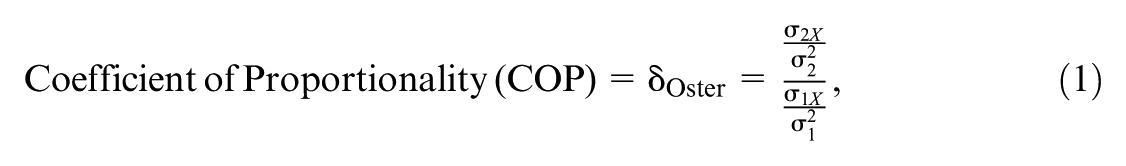
Altonji et al. (2005) established the basis for Oster’s COP by expressing the dual components of confounding in terms of commonly used two-stage econometric techniques—one stage to predict the outcome, Y, and a second to predict selection into the focal predictor, X. Formally, let W₁ represent the prediction of the outcome Y based on observed covariates Z, and W₂ the prediction of Y based on unobserved covariates CV. Noting selection bias occurs when “… the treatment or control status of subjects is related to unmeasured characteristics that themselves are related to the outcome…” (Barnow et al., 1980, p. 1), a key contribution of Altonji et al. (2005) was to use a logistic regression to benchmark how strong selection into the focal predictor X (e.g., a treatment) based on W₂ must be relative to selection based on W₁ to nullify the estimated effect of X on Y (for other benchmarking techniques, see Rosenbaum, 1986; Cinelli & Hazlett, 2020; Frank, 2000; Veitch & Zaveri, 2020). Applying this insight to their empirical analysis of the effect of attending a Catholic school on student outcomes, Altonji et al. (2005, p. 176) concluded that, “the normalized shift in the distribution of the unobservables [selection based on W₂] would have to be 3.55 times as large as the shift in the observables [selection based on W₁] to explain away the entire CH [Catholic High School] effect. This seems highly unlikely.”

Based on Altonji et al.’s (2005) formulation, Oster (2019, p. 192) expressed the COP in a fully linear framework as:

Coefficient of Proportionality (COP) = δ_{Oster} = \frac{\frac{σ_{2 X}}{σ_{2}^{2}}}{\frac{σ_{1 X}}{σ_{1}^{2}}},

(1)

where $σ_{2 X}$ is the covariance between X and W₂, and $σ_{2}^{2}$ is the variance of W₂. Similarly, $σ_{1 X}$ is the covariance between X and W₁ and $σ_{1}^{2}$ is the variance of W₁. Therefore, the COP can be can be interpreted as the ratio of the prediction of X based on the unobserved covariates $(\frac{σ_{2 X}}{σ_{2}^{2}})$ to the prediction based on the observed covariates $(\frac{σ_{1 X}}{σ_{1}^{2}})$ , accounting for the relationships to Y through W₁ and W₂. Moreover, because W₁ and W₂ are defined in the prediction of Y, they express the observed and unobserved covariates on a common scale defined by the variance of Y.

2.2 Estimation of δ_oster

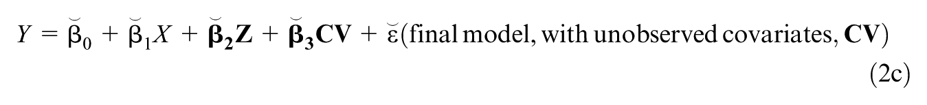
Oster (2019) developed an estimator for δ_oster based on coefficient stability observed by an analyst across the following three models estimated from a sample:

Y = {\overset{\cdot}{β}}_{0} + {\overset{\cdot}{β}}_{1} X + \overset{\cdot}{ε} (unconditional baseline model)

(2a)

Y = {\tilde{β}}_{0} + {\tilde{β}}_{1} X + {\tilde{β}}_{2} Z + \tilde{ε} (intermediate model with observed covariates, Z)

(2b)

Y = {\overset{⌣}{β}}_{0} + {\overset{⌣}{β}}_{1} X + {\overset{⌣}{β}}_{2} Z + {\overset{⌣}{β}}_{3} C V + \overset{⌣}{ε} (final model, with unobserved covariates, C V)

(2c)

There are no distributional assumptions about the error terms (ε) in each model except when defining a threshold for decision-making based on statistical significance (see Subsection 7.3).

Note that each model in Equation 2 is conceptualized in terms of estimated values represented by ^., ~, or ⏝ depending on the covariates an analyst adds, or considers adding, to the model. But each model has a population analog. For example, the population analog for Equation 2c is $Y = β_{0} + β_{1} X + β_{2} Z + β_{3} CV + ε$ with β₁ representing the effect of X on Y conditioning on observed and unobserved covariates in the population. If one also considered the observed covariates to be sampled from a set of covariates (e.g., Altonji et al., 2005) then only Equation 2c would be a true population model assuming that the union of Z and CV is the population of covariates.

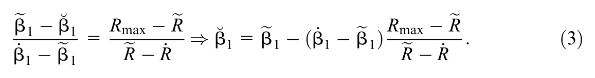
Oster (2019) used the change in estimated effect from $\overset{\cdot}{β}$ ₁ to ${\tilde{β}}_{1}$ from Equation 2a to Equation 2b and corresponding change in explained variance (aka the coefficient of determination, R²) to estimate δ_oster. To represent Oster’s estimation strategy, first define $\overset{\cdot}{R}$ ² as the R² for Equation 2a and ${\tilde{R}}^{2}$ as the R² for Equation 2b. Importantly, Oster’s derivation assumed a maximum $R^{2}$ (R_max) in the final model in Equation 2c that could be less than one. Consistent with challenges to determinism based on human agency and free will (e.g., Strawson, 2008), some variance in the outcome may be unexplainable even accounting for all conceivable observed and unobserved covariates (Oster, p. 201, developed an empirical guideline for R_max based on randomized studies see Subsection 8.1.2). Using these quantities, Oster derived an intuitive estimator for β₁ in Equation 2c:

\frac{{\tilde{β}}_{1} - {\overset{⌣}{β}}_{1}}{{\dot{β}}_{1} - {\tilde{β}}_{1}} = \frac{R_{\max} - \tilde{R}}{R - \dot{R}} \Rightarrow {\overset{⌣}{β}}_{1} = {\tilde{β}}_{1} - ({\dot{β}}_{1} - {\tilde{β}}_{1}) \frac{R_{\max} - \tilde{R}}{\tilde{R} - \dot{R}} .

(3)

The estimator leverages intuition based on coefficient stability: “the ratio of the movement in coefficients $[\frac{{\tilde{β}}_{1} - {\overset{⌣}{β}}_{1}}{{\overset{\cdot}{β}}_{1} - {\tilde{β}}_{1}}]$ is equal to the ratio of the movement in R-squared $[\frac{R_{\max} - \tilde{R}}{\tilde{R} - \overset{\cdot}{R}}]$ ” (Oster, 2019, p. 193).

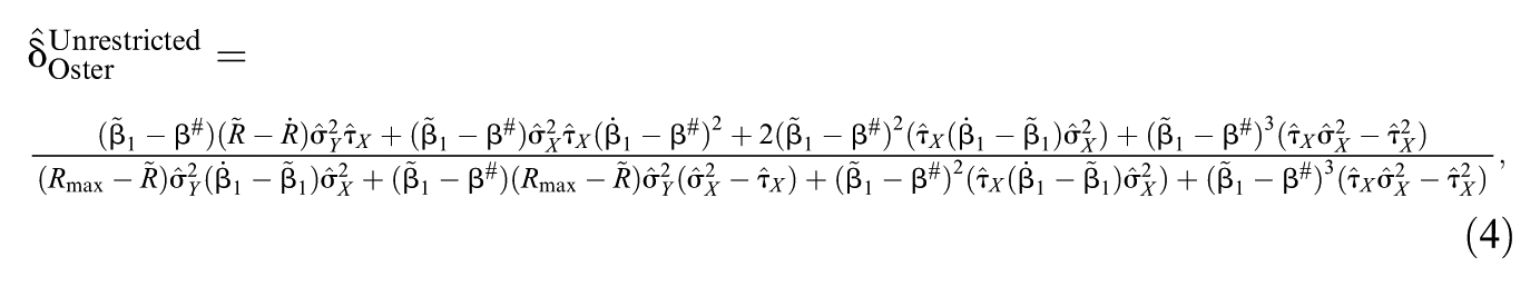
While the expression in Equation 3 is intuitive, it is restricted by the assumption that selection on unobserved covariates equals selection on observed covariates (it is also restricted by the assumption that the relative contribution of each unobserved covariate to X is the same as its contribution to Y, which we will discuss in Subsection 7.1). Oster relaxed the two assumptions to derive an unrestricted estimator for β₁ as a function of δ_Oster defined in Equation 1. This allowed Oster to create a sensitivity index by identifying the value of δ_Oster that would generate a specified value of ${\overset{⌣}{β}}_{1}$ .

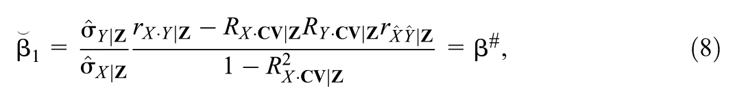
Specifically, Oster (2019) solved three equations for three unknowns (based on the stability of estimated effects and R² across the models in Equation 2) to derive an expression to estimate δ_Oster that would generate a threshold value of ${\overset{⌣}{β}}_{1}$ = β ^# for a specified R_max yielding:

{\hat{δ}}_{Oster}^{Unrestricted} = \frac{\begin{matrix} ({\tilde{β}}_{1} - β^{#}) (\tilde{R} - \overset{\cdot}{R}) {\hat{σ}}_{Y}^{2} {\hat{τ}}_{X} + ({\tilde{β}}_{1} - β^{#}) {\hat{σ}}_{X}^{2} {\hat{τ}}_{X} ({\overset{\cdot}{β}}_{1} - β^{#})^{2} + 2 ({\tilde{β}}_{1} - β^{#})^{2} ({\hat{τ}}_{X} ({\overset{\cdot}{β}}_{1} - {\tilde{β}}_{1}) {\hat{σ}}_{X}^{2}) + ({\tilde{β}}_{1} - β^{#})^{3} ({\hat{τ}}_{X} {\hat{σ}}_{X}^{2} - {\hat{τ}}_{X}^{2}) \end{matrix}}{\begin{matrix} (R_{max} - \tilde{R}) {\hat{σ}}_{Y}^{2} ({\overset{\cdot}{β}}_{1} - {\tilde{β}}_{1}) {\hat{σ}}_{X}^{2} + ({\tilde{β}}_{1} - β^{#}) (R_{max} - \tilde{R}) {\hat{σ}}_{Y}^{2} ({\hat{σ}}_{X}^{2} - {\hat{τ}}_{X}) + ({\tilde{β}}_{1} - β^{#})^{2} ({\hat{τ}}_{X} ({\overset{\cdot}{β}}_{1} - {\tilde{β}}_{1}) {\hat{σ}}_{X}^{2}) + ({\tilde{β}}_{1} - β^{#})^{3} ({\hat{τ}}_{X} {\hat{σ}}_{X}^{2} - {\hat{τ}}_{X}^{2}) \end{matrix}},

(4)

where ${\hat{τ}}_{X}$ is the estimated residual variance in X after conditioning on Z. Note that β ^# may equal zero nullifying the estimated effect, but it also may be a non-zero threshold for inference. Most importantly, ${\hat{δ}}_{Oster}^{Unrestricted}$ is an index of sensitivity. The larger the value of ${\hat{δ}}_{Oster}^{Unrestricted}$ necessary to reduce ${\tilde{β}}_{1}$ to β ^# (for specified R _max ), the more robust the inference regarding β₁.

2.3 Example Application: Effect of Low Birthweight and Preterm on Infant IQ

To illustrate the use of the COP throughout the article, we focus on the most robust inference (defined by ${\hat{δ}}_{Oster}^{Unrestricted}$ ) among the examples used in Oster (2019, Table 3, Panel A, Column 3), regarding the effect of Low birthweight and preterm on infant IQ. The inference is of scientific importance representing the implications of birth conditions throughout schooling and the life course (e.g., Breslau et al., 1994). Furthermore, if Low birthweight and preterm affect IQ, then policy might attend more fully to corresponding prenatal medical and postnatal educational supports (Gross et al., 1997; National Research Council, 2000).

For the baseline model (Equation 2a, including the covariates age and child female), Oster reported ${\overset{\cdot}{β}}_{1}$ = −.188, and ${\overset{\cdot}{R}}^{2}$ = .004. For the intermediate model (Equation 2b, including five additional covariates: mother Black; mother age; mother education; mother income; mother married), Oster reported ${\tilde{β}}_{1} = - . 125$ and ${\tilde{R}}^{2} = . 251$ . For the final model Equation 2c, Oster specified β ^# = 0 and $R^{2} = R_{max} = . 61$ . Based on these values, Oster reported ${\hat{δ}}_{Oster}^{Unrestricted}$ = 1.37 based on Equation 4 indicating that selection on the unobserved covariates would have to be more than one-third stronger than selection on the observed covariates to reduce ${\overset{⌣}{β}}_{1}$ to 0 with $R^{2}$ of .61.¹

3. Critiques of Oster’s COP (δ_Oster)

In this section, we present details of the critiques of Oster (2019). The first critique of Oster (2019) is based on Cinelli and Hazlett (2020) regarding the definition of δ_Oster based on Altonji et al. (2005) through a two-stage process as in Equation 1. In the first stage, Cinelli and Hazlett (2020) considered the following model for a scalar observed covariate Z and a scalar unobserved covariate CV:

Y = β_{1} X + W_{1} + W_{2} = β_{1} X + ψ Z + γ CV,

where W₁ = $ψ$ Z and W₂ = γCV. Note that technically Oster considers W₂ as wholly representing the unobserved covariate without a parameter (i.e., $γ$ = 1), but we use Cinelli and Hazlet’s formulation W₂ = $γ$ CV.

Then Cinelli and Hazlett (2020) defined the model for selection into X as:

X = θ W_{1} + λ W_{2},

with W₁ and W₂ already representing the relationships of the covariates to Y (through $ψ$ and γ). Using the previous two expressions for Y and X, Cinelli and Hazlett (2020, Equation 27, p. 64) then re-express δ_Oster:

δ_{Oster} = \frac{\frac{λ}{θ}}{\frac{γ}{ψ}} = \frac{λ ψ}{θ γ}

The middle expression shows how Oster’s formulation of the COP scales selection on unobserved covariates (λ) to that on observed covariates (θ) relative to their corresponding contributions to Y (through γ and ψ). Cinelli and Hazlett then showed that representing the dual relationships associated with a confounder through the two sets of coefficients for Y and X can lead to counter-intuitive results. Consider $ψ$ = $θ$ = q and $λ = γ$ = q/2 (where q is any real number) in which case selection on the CV (λ = q/2) is half that of selection on Z (θ = q), but δ_Oster = 1 (Basu, 2023, p. 10 draws the corresponding conclusion that a benchmark of δ_Oster = 1 is problematic).²

The second critique of Oster (2019) is based on ${\hat{δ}}_{Oster}^{Unrestricted}$ as an estimator for δ_Oster (Masten & Poirier, 2022). The expression for ${\hat{δ}}_{Oster}^{Unrestricted}$ in Equation 4, based on solving a system of three equations in three unknowns, yields cubic dependence on both β ^# and ${\tilde{β}}_{1}$ . As a result, the dependence of ${\hat{δ}}_{Oster}^{Unrestricted}$ on β ^# is non-monotonic and may exhibit discontinuities. Specifically, Masten and Poirier (2022) showed that the value of ${\hat{δ}}_{Oster}^{Unrestricted}$ necessary to produce a sign change can be different from, and smaller than, the value of ${\hat{δ}}_{Oster}^{Unrestricted}$ necessary to nullify the estimated effect by making it equal to zero. This is counterintuitive; someone seeking to reduce the estimated effect of ${\tilde{β}}_{1}$ to zero might perceive an inference to be highly robust, while someone seeking the more extreme reversal of sign (even just to an estimate of small magnitude but opposite sign than ${\tilde{β}}_{1}$ ) might perceive the inference to be fragile (see Masten & Poirier, 2022, p. 3; see also Basu, 2023).

4. Recasting the COP in a Correlational Framework: δ_Correlation

In this section, we present a definition and estimator of a correlation-based COP, δ_Correlation, that address the critiques of Oster (2019).

4.1 Notation

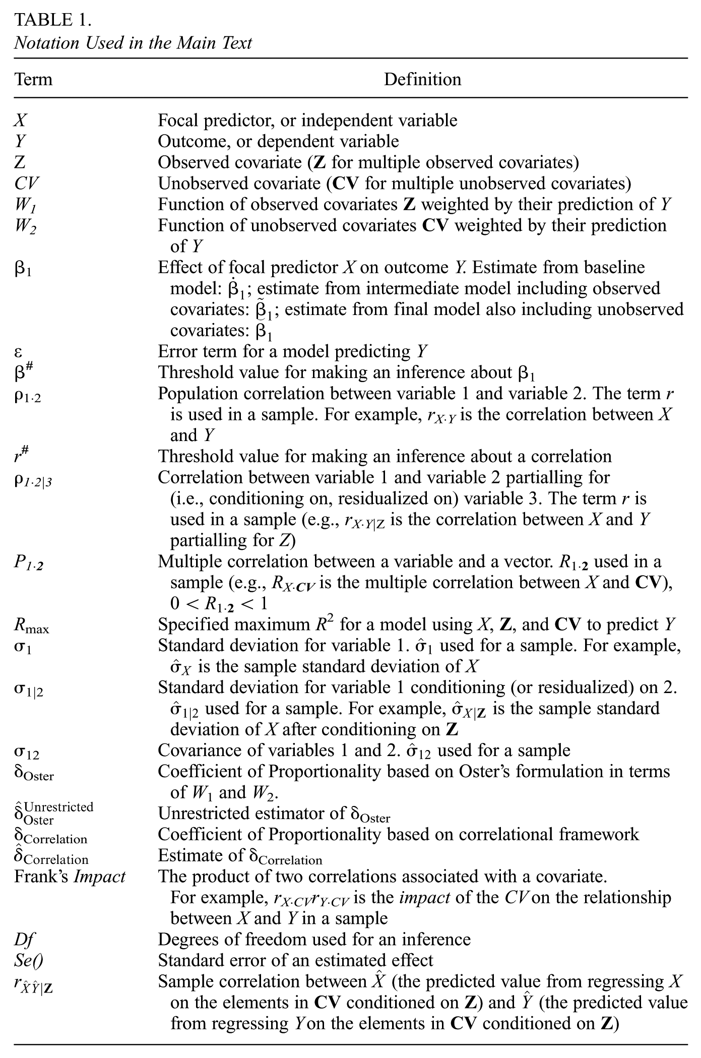
Following the presentation of Oster’s COP, we use Greek letters to represent population parameters that define δ_Correlation. We use ^ to represent an estimated value with two exceptions. First, we use ^., ~, and ⏝ to differentiate among the estimates in Equation 2. Second, following convention, we use r to represent a sample correlation between two scalars. To be consistent, we use $R_{Y \cdot X Z}^{2}$ to represent the coefficient of determination from model Equation 2b in a sample including the observed covariates Z, equivalent to Oster’s $\tilde{R}$ ; and we use $R_{Y \cdot X ZCV}^{2}$ = $R^{2}$ to represent the coefficient of determination from model Equation 2c also including the unobserved covariates CV. We then use “|” to represent partialled for, or residualized on (Cinelli & Hazlett, 2020, p. 48). For example, r_X·Y| _Z represents the sample correlation between X and Y partialled for, or residualized on, the observed covariates Z. Also using the “|”, ${\hat{σ}}_{X | Z}$ represents the sample standard deviation of X conditional on Z and ${\hat{σ}}_{Y | Z}$ represents the sample standard deviation of Y conditional on Z. See Table 1 for the notation used throughout.

Table 1.

Notation Used in the Main Text

Term	Definition
X	Focal predictor, or independent variable
Y	Outcome, or dependent variable
Z	Observed covariate (Z for multiple observed covariates)
CV	Unobserved covariate (CV for multiple unobserved covariates)
W ₁	Function of observed covariates Z weighted by their prediction of Y
W ₂	Function of unobserved covariates CV weighted by their prediction of Y
β₁	Effect of focal predictor X on outcome Y. Estimate from baseline model: ${\overset{\cdot}{β}}_{1}$ ; estimate from intermediate model including observed covariates: ${\tilde{β}}_{1}$ ; estimate from final model also including unobserved covariates: ${\overset{⌣}{β}}_{1}$
ε	Error term for a model predicting Y
β ^#	Threshold value for making an inference about β₁
ρ_1·2	Population correlation between variable 1 and variable 2. The term r is used in a sample. For example, r_X·Y is the correlation between X and Y
r ^#	Threshold value for making an inference about a correlation
ρ _1·2\|3	Correlation between variable 1 and variable 2 partialling for (i.e., conditioning on, residualized on) variable 3. The term r is used in a sample (e.g., r_X·Y\|Z is the correlation between X and Y partialling for Z)
P _1· ₂	Multiple correlation between a variable and a vector. R_1· ₂ used in a sample (e.g., R_X· _CV is the multiple correlation between X and CV), 0 < R_1· ₂ < 1
R _max	Specified maximum R² for a model using X, Z, and CV to predict Y
σ₁	Standard deviation for variable 1. ${\hat{σ}}_{1}$ used for a sample. For example, ${\hat{σ}}_{X}$ is the sample standard deviation of X
σ_1\|2	Standard deviation for variable 1 conditioning (or residualized) on 2. ${\hat{σ}}_{1 \| 2}$ used for a sample. For example, ${\hat{σ}}_{X \| Z}$ is the sample standard deviation of X after conditioning on Z
σ₁₂	Covariance of variables 1 and 2. ${\hat{σ}}_{12}$ used for a sample
δ_Oster	Coefficient of Proportionality based on Oster’s formulation in terms of W₁ and W₂.
${\hat{δ}}_{Oster}^{Unrestricted}$	Unrestricted estimator of δ_Oster
δ_Correlation	Coefficient of Proportionality based on correlational framework
${\hat{δ}}_{Correlation}$	Estimate of δ_Correlation
Frank’s Impact	The product of two correlations associated with a covariate. For example, r_X·CVr_Y·CV is the impact of the CV on the relationship between X and Y in a sample
Df	Degrees of freedom used for an inference
Se()	Standard error of an estimated effect
$r_{\hat{X} \hat{Y} \| Z}$	Sample correlation between $\hat{X}$ (the predicted value from regressing X on the elements in CV conditioned on Z) and $\hat{Y}$ (the predicted value from regressing Y on the elements in CV conditioned on Z)

4.2 Definition of δ_Correlation

As we noted in presenting the intuition behind Oster’s COP, one of Oster’s (2019) contributions was to express the COP in terms of OLS estimates of the General Linear Model (GLM). Correspondingly, our COP is conceptualized in terms of the linear relationships among the focal predictor, outcome, and covariates, and we assume OLS will be used to estimate the GLMs in Equation 2. This allows us to derive closed form expressions for the relevant correlations and COP.³

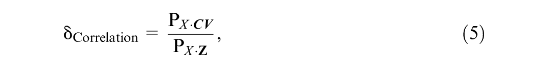
Specifically, we define δ_Correlation as the ratio of two (multiple) correlations:

δ_{Correlation} = \frac{P_{X \cdot CV}}{P_{X \cdot Z}},

(5)

where of P_X· _CV represents the population correlation (the square root of the coefficient of determination) between X and the vector CV and P_X· _Z represents the population multiple correlation between X and Z. For the square root of coefficients of determination, we assume 0 < P_X· _CV < 1 and 0 < P_X· _Z < 1 to ensure the directionality of the impact on β₁ (Frank, 2000).

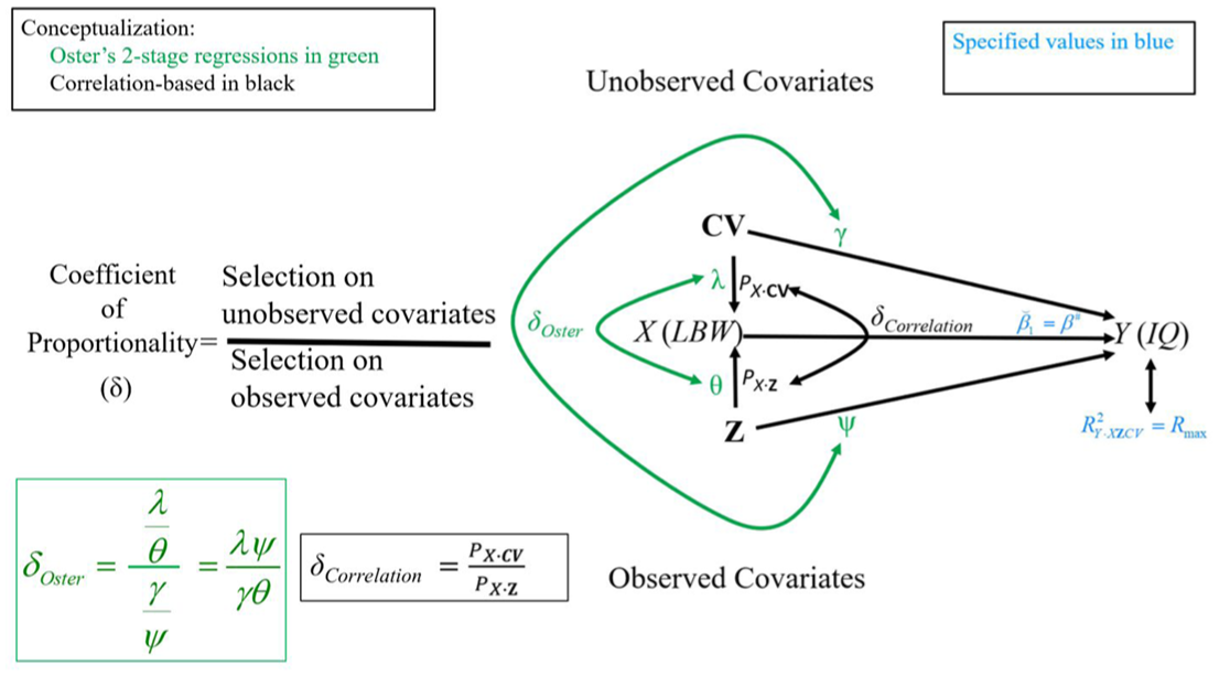
The difference in conceptualization between δ_Oster and δ_Correlation is shown in Figure 1. The core of the figure features a Directed Acyclic Graph (e.g., Pearl, 2009) focusing on the effect of X on Y, with observed covariates Z at the bottom and unobserved covariates CV at the top. Note that arrows lead from both sets of covariates to X and Y indicating Z and CV are causally prior to X and Y at the bottom left of Figure 1. Both δ_Oster and δ_Correlation are defined by the ratio of selection on unobservables (CV) to selection on observables (Z). But δ_Oster is conceived through a two-stage approach, ultimately expressing selection into the treatment (X) through λ and θ scaled by each set of variables’ relationships to Y (defining γ and ψ in Section 3). This creates the counterintuitive results noted by Cinelli and Hazlett (2020). In contrast, δ_Correlation is a function only of scale-free correlations between X and its predicted values based on CV or Z. Selection on unobserved covariates is twice as strong as on observed covariates if P_X· _CV is twice as large as P_X· _Z . Although P_X· _CV and P_X· _Z are not directly functions of associations with Y, we will show in Supplemental Appendices A and B that, for a given correlation between X and CV, the relationship of CV to the outcome Y (P_Y·CV) is essentially determined by specification of R_max. Furthermore, in Supplemental Appendix C, we verify that our correlational framework can reproduce the data generated through Oster’s two-stage process, showing how a correlation-based formulation accounts for differences in variances of covariates that motivated Oster’s (2019, pp. 189–192) formulation. The two correlations associated with the CV can be recombined through the product P_X·CV P_Y·CV, which Frank (2000) referred to as the impact of a confounding variable. Finally, the scalar results can be generalized to multiple observed covariates as in Subsection 7.1.

Figure 1.

Difference in conceptualizations of the coefficient of proportionality: δ_Oster versus δ_Correlation.

4.3 Initial Assumptions for Estimation

We make four assumptions for our initial derivation of an expression for $\hat{δ}$ _Correlation to estimate δ_Correlation. The first assumption simply explicates a characteristic of the unobserved covariates as confounders. The next two assumptions state stronger conditions which we relax in Section 7. The final assumption concerns the evaluation of an estimated effect relative to an absolute threshold rather one based on sampling variability, which we also relax in Section 7.

The first assumption is that $R_{Y \cdot CV | Z}^{2} > 0$ . That is, that the unobserved covariates add explanatory power to Y after residualizing on Z. This assumption is consistent with conceptualizations of the elements in CV as omitted confounding variables that are related to Y as well as to X (Barnow, Cain & Goldberger, 1980; Frank, 2000; Oster, 2019). Implied by $R_{Y \cdot CV | Z}^{2} > 0$ is that ${\hat{σ}}_{Y | Z}$ > 0 (at least some variance in Y is not explained by Z). This assumption is required for the general calculation of $\hat{δ}$ _Correlation to yield real numbers (Supplemental Appendix A) as well as to establish that the relationship between $\hat{δ}$ _Correlation and ${\overset{⌣}{β}}_{1}$ is continuous and strictly negatively monotonic (Supplemental Appendix D).

Second, in initial derivations, we treat CV as a single covariate, CV. Like any variable in a model, the CV may be a weighted combination of variables. Moreover, in Subsection 7.1, we show that using a single CV defined as an index of multiple unobserved covariates weighted by their relative contributions to the outcome (W₂) is conservative in terms of avoiding overstating the robustness of the inference, protecting the null hypothesis of zero effect.

Third, we assume CV is orthogonal to the elements in Z, expressed as R_CV· _Z = 0 (see Oster, 2019, p. 192). Intuitively, if R_CV· _Z ≠ 0, then some of the impact of the unobserved covariate CV on the estimate of β₁ would be accounted for by the observed covariates in Z, weakening the challenge to the inference based on omission of the CV (Frank, 2000). In the empirical example, the relationship between Low birthweight and preterm (X) on IQ (Y) might be challenged based on an unobserved covariate of caloric intake (CV—Kramer, 1987). But the challenge is weaker if caloric intake is already partly accounted for by measured covariates including income and education (Z). Following Mauro’s (1990, p. 316) intuition: “clearly, the effect of omitting CV on the regression coefficient of the primary predictor (X) is much greater when the correlation between the omitted variable and the covariates is small.” In Subsection 7.2, we show that assuming R_CV· _Z = 0 is generally conservative in terms of protecting the null hypothesis.

Fourth, in initial derivations, we assume that the threshold for inference, β ^# , is specified independent of statistical inference based on a standard error. In Subsection 7.3, we leverage our correlational framework to develop expressions for r_X· _CV _|Z and r_Y· _CV _|Z required to nullify the statistical inference for β₁, accounting for the change in standard error as well as in the estimated effect if an unobserved covariate were added to a model.

4.4 Estimation of δ_Correlation

Oster’s (2019) expression in Equation 4 for ${\hat{δ}}_{Oster}^{Unrestricted}$ based on solving three equations for three unknowns exhibits a non-monotonic relationship between ${\hat{δ}}_{Oster}^{Unrestricted}$ and the corresponding estimate of $β_{1}$ as critiqued by Masten and Poirier (2022). We address this critique by deriving expressions for the COP that satisfy two fundamental relations:

{\overset{⌣}{β}}_{1} = β^{#}

(6a)

R_{Y \cdot X Z CV}^{2} = R_{\max} .

(6b)

The relation in Equation 6a, defines a threshold for an inference, β ^# , such that an inference based on the intermediate regression in Equation 2b is invalid if ${\overset{⌣}{β}}_{1}$ in Equation 2c is less than or equal to β ^# . The relation in Equation 6b indicates that the total variance in Y explained by X, Z, and CV in Equation 2c has a maximum value that may be less than one: $R_{Y \cdot X Z CV}^{2}$ = R_max, R_max < 1 (this includes Altonji et al.’s, 2005, special case of R_max = 1). The relationships in Equation 6 thus represent Oster’s (2019, p. 198) goal to identify “…the value of δ [COP] that would produce β = 0 [β ^# = 0] under the assumed R_max….”

Proposition 1. Define

{\hat{δ}}_{Correlation} = \frac{r_{X \cdot CV}}{R_{X \cdot Z}} = \frac{\sqrt{1 - R_{X \cdot Z}^{2}} (r_{X \cdot Y | Z} - \frac{{\hat{σ}}_{X | Z}}{{\hat{σ}}_{Y | Z}} β^{#})}{R_{X \cdot Z} \sqrt{\frac{{\hat{σ}}_{X | Z}^{2}}{{\hat{σ}}_{Y | Z}^{2}} {β^{#}}^{2} - 2 r_{X \cdot Y | Z} \frac{{\hat{σ}}_{X | Z}}{{\hat{σ}}_{Y | Z}} β^{#} + \frac{R_{max} - R_{Y \cdot Z}^{2}}{(1 - R_{Y \cdot Z}^{2})}}} .

(7)

Under this definition, ${\hat{δ}}_{Correlation} \overset{P}{\to} δ_{Correlation}$ . That is, that ${\hat{δ}}_{Correlation}$ is a consistent estimator of δ_Correlation.

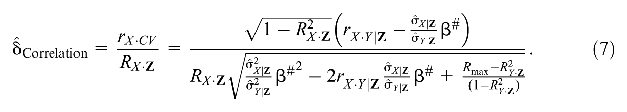
Proof. As in Supplemental Appendix A, we first use the Frisch–Waugh–Lovell (Frisch & Waugh, 1933; Lovell, 1963) decomposition to condition all terms in Equation 2c on Z. We then express the two relations in Equation 6 for ${\overset{⌣}{β}}_{1}$ and $R_{Y \cdot X Z CV}^{2}$ as functions of two unknowns associated with the unobserved confounding variable CV: $r_{X \cdot CV | Z} and r_{Y \cdot CV | Z}$ . Solving the two equations for two unknowns yields an expression for $r_{X \cdot CV | Z}$ that we then use to obtain $r_{X \cdot CV} = \sqrt{1 - R_{X \cdot Z}^{2}} r_{X \cdot CV | Z}$ based on Supplemental Appendix B (under the assumption that the observed and unobserved covariates are orthogonal, which is relaxed in Subsection 7.2). Then ${\hat{δ}}_{Correlation} = \frac{r_{X \cdot CV}}{R_{X \cdot Z}}$ is obtained by dividing $r_{X \cdot CV}$ by the sample quantity $R_{X \cdot Z}$ . Given the properties of OLS estimates (e.g., Johnson & Wichern, 2002, p. 151), $r_{X \cdot CV} \overset{P}{\to} ρ_{X \cdot CV}$ and $R_{X \cdot Z} \overset{P}{\to} P_{X \cdot Z}$ ; therefore, ${\hat{δ}}_{Correlation} \overset{P}{\to} δ_{Correlation}$ .

The expression in Equation 7 shows the relationship between $\hat{δ}$ _Correlation and R_max (the targeted value of $R_{Y \cdot X Z CV}^{2}$ ). Specifically, the larger the value of R_max the smaller the $\hat{δ}$ _Correlation and the less the selection on the unobserved covariate (r_X·CV) relative to on observed covariates (R_X· _Z ) required to nullify the inference regarding β₁. In the birthweight example, the larger the expected final variance in IQ that could be explained by observed and unobserved covariates, the less the relative selection into Low birthweight and preterm on the unobserved covariate necessary to nullify the estimated effect on IQ. Correspondingly, the larger the value of R_max, the less robust the inference regarding β₁. This implies that specifying R_max < 1 may allow interpreters of an inference to identify when there may be enough evidence to act pragmatically even if all is not, or cannot be, known about a phenomenon (Frank et al., 2023, Holland, 1986).

We have already shown how the definition of δ_Correlation addresses Cinelli and Hazlett’s (2020) critique of δ_Oster by expressing the COP in terms of scale-free correlations. The expression for $\hat{δ}$ _Correlation in Equation 7 then addresses Masten and Poirier’s (2022) critique of Oster (2019) because $\hat{δ}$ _Correlation is a continuous and monotonic (quadratic) function of ${\overset{⌣}{β}}_{1}$ assuming $r_{Y \cdot CV | Z}^{2} > 0$ (Supplemental Appendix D). That is, the values of $\hat{δ}$ _Correlation associated with the smallest possible difference between ${\tilde{β}}_{1}$ and ${\overset{⌣}{β}}_{1}$ creating a sign change are adjacent to the values that reduce ${\overset{⌣}{β}}_{1}$ to zero. Therefore, someone seeking to change the sign of the estimated effect would have a similar sense of the robustness as someone seeking to nullify the estimated effect.

Note that our calculation of $\hat{δ}$ _Correlation depends only on the specified values of R_max and β ^# , the sample correlations r_X·Y| _Z , R_X· _Z , and R_Y· _Z , as well as the sample ratio $\frac{{\hat{σ}}_{X | Z}}{{\hat{σ}}_{Y | Z}}$ (for β ^# = 0, $\frac{{\hat{σ}}_{X | Z}}{{\hat{σ}}_{Y | Z}}$ is not needed). That is, unlike ${\hat{δ}}_{Oster}^{Unrestricted}$ , our COP $\hat{δ}$ _Correlation does not depend on an analyst’s subjective choice of baseline model. As we show in the empirical example and simulations below, ${\hat{δ}}_{Oster}^{Unrestricted}$ and the corresponding interpretation of an inference can be highly sensitive to the choice of baseline model, a point we return to in Subsection 8.1.3.

4.5 Verification of $\hat{δ}$ _Correlation Through Simulation

In Supplemental Appendix E, we use simulated data to verify the set of expressions for r_X·CV| _Z and r_Y·CV| _Z (used to generate $\hat{δ}$ _Correlation) in scenarios in which the exact results are known across 36 scenarios generated by varying values of β ^# , $R_{Y \cdot X Z}^{2}$ ( $\tilde{R}$ ), ${\tilde{β}}_{1}$ , and $R_{Y \cdot X Z CV}^{2}$ ( $R^{2}$ or Oster’s R_max). For results, all the calculated values of ${\overset{⌣}{β}}_{1}$ were within .001 of the specified β ^# and the calculated values of $R_{Y \cdot X Z CV}^{2}$ were all within .001 of the specified values of R_max using the Lavaan procedure in R (used for generating OLS estimates of linear models from covariance matrices—Rosseel, 2012). The results were even more accurate if we calculated ${\overset{⌣}{β}}_{1}$ and $R_{Y \cdot X Z CV}^{2}$ using direct function based on Supplemental Appendix A. Thus, the results in Supplemental Appendix E verify the closed form expressions for r_X·CV| _Z and r_Y·CV| _Z to produce the specified values of β ^# and R_max in Equations 6a and 6b.

The full set of simulation results in Supplemental Table E1 help us interpret the expression for $\hat{δ}$ _Correlation in Equation 7. Confirming our interpretation of Equation 7, the smaller the R_max, the larger the value of $\hat{δ}$ _Correlation. Inferences may be interpreted as more robust when not all of the variance in an outcome can be explained. Furthermore, although Equation 7 is not a direct function of ${\tilde{β}}_{1}$ , Table E1 reveals that the greater the difference between ${\tilde{β}}_{1}$ and β ^# , the larger the value of $\hat{δ}$ _Correlation, reflective of the stronger covariate necessary to nullify the inference when ${\tilde{β}}_{1}$ far exceeds the threshold for inference (β ^# ).

5. Application of δ_Correlation: Estimated Effect of Low Birthweight and Preterm Status on IQ

In this section, we apply our correlation-based framework to the example of the effect of Low Birthweight and Preterm Status on IQ,⁴ and we recover the correlations that combine through their product to define the impact of the of the unobserved covariate on the estimated effect.

5.1 Calculation of $\hat{δ}$ _Correlation

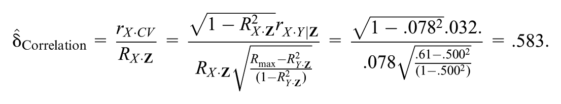
We calculate $\hat{δ}$ _Correlation for the running example of the estimated effect of Low birthweight and preterm on IQ based on conventionally reported quantities in Oster (2019). We also show how the relations defined in Equation 6 are satisfied through the dual components of the CV—the correlation with X and the correlation with Y (corresponding commands and output for the Konfound packages in Stata and R are provided in Supplemental Appendix F). In Supplemental Appendix G, we calculate: $R_{X \cdot Z} = . 078; r_{X \cdot Y | Z} = . 032; and R_{Y \cdot Z} = . 500$ based on Oster’s reported quantities of $S e ({\tilde{β}}_{1})$ =.05049 (italicized digits inferred—see Supplemental Appendix G), $R_{Y \cdot X Z}^{2} = {\tilde{R}}^{2}$ = .251, ${\hat{σ}}_{X} = . 217$ , ${\hat{σ}}_{Y} = . 991$ , and df = 6,165. Then from Equation 7, for the specified β ^# = 0:

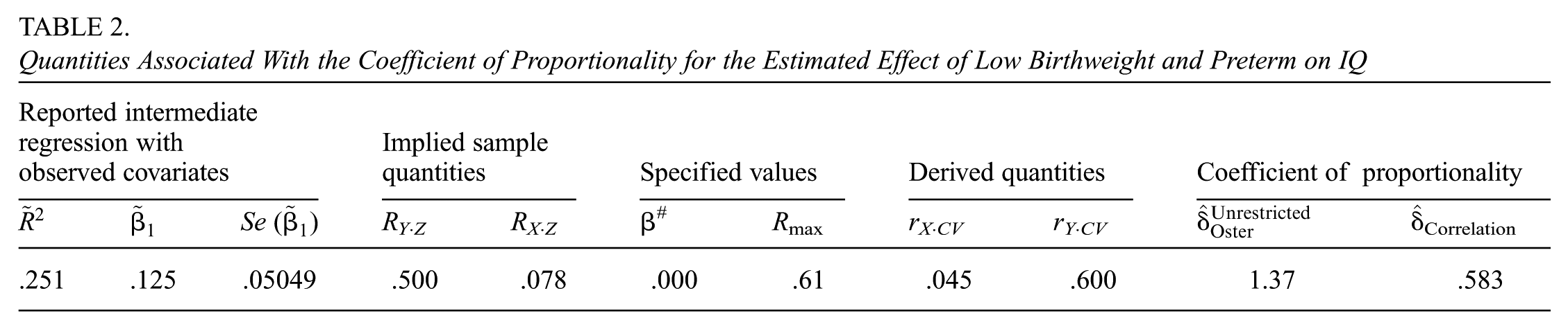
{\hat{δ}}_{Correlation} = \frac{r_{X \cdot CV}}{R_{X \cdot Z}} = \frac{\sqrt{1 - R_{X \cdot Z}^{2}} r_{X \cdot Y | Z}}{R_{X \cdot Z} \sqrt{\frac{R_{max} - R_{Y \cdot Z}^{2}}{(1 - R_{Y \cdot Z}^{2})}}} = \frac{\sqrt{1 - . 078^{2}} . 032 .}{. 078 \sqrt{\frac{. 61 - . 500^{2}}{(1 - . 500^{2})}}} = . 583 .

The correlation between an unobserved covariate and Low birthweight and preterm would have to be about 58% that of the very modest multiple correlation associated with the observed covariates (R_X· _Z = .078) to nullify the estimated effect of Low birthweight and preterm on IQ for specified R_max = .61. We note this result is obtained under the assumption that the unobserved covariates are orthogonal to the observed covariates (R_CV· _Z = 0). But in Supplemental Appendix H, we show that for $\hat{δ}$ _Correlation < 1 as in this example, there is no value of R_CV· _Z that would make $\hat{δ}$ _Correlation smaller; $\hat{δ}$ _Correlation = .583 is a conservative expression of the robustness of the inference. A summary of reported, implied, specified, and derived quantities as well as the COPs is provided in Table 2.

Table 2.

Quantities Associated With the Coefficient of Proportionality for the Estimated Effect of Low Birthweight and Preterm on IQ

Reported intermediate regression with observed covariates			Implied sample quantities		Specified values		Derived quantities		Coefficient of proportionality
${\tilde{R}}^{2}$	${\tilde{β}}_{1}$	Se ( ${\tilde{β}}_{1}$ )	R _Y·Z	R _X·Z	β ^#	R _max	r _X·CV	r _Y·CV	${\hat{δ}}_{Oster}^{Unrestricted}$	$\hat{δ}$ _Correlation
.251	.125	.05049	.500	.078	.000	.61	.045	.600	1.37	.583

5.2 Recovery of r_X·CV and r_Y·CV Defining the Impact of the Confounding Variable

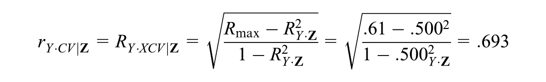
To better interpret the two components of confounding in the empirical example, we recover r_X·CV and r_Y·CV from $\hat{δ}$ _Correlation. First, from Equation 7, $r_{X \cdot CV} = {\hat{δ}}_{Correlation} R_{X \cdot Z} = (. 58330) . 07776 = . 04536$ . Then, for ${\overset{⌣}{β}}_{1}$ = β ^# = 0 model (Equation 2b) reduces to $Y | Z = {\overset{⌣}{β}}_{0} + {\overset{⌣}{β}}_{3} C V | Z + \overset{⌣}{ε}$ . Therefore, all the variance explained in Y|Z is due to CV|Z and:⁵

r_{Y \cdot CV | Z} = R_{Y \cdot XCV | Z} = \sqrt{\frac{R_{\max} - R_{Y \cdot Z}^{2}}{1 - R_{Y \cdot Z}^{2}}} = \sqrt{\frac{. 61 - . 500^{2}}{1 - . 500_{Y \cdot Z}^{2}}} = . 693

Under the assumption that R_CV· _Z = 0, $r_{Y \cdot CV} = \sqrt{1 - R_{Y \cdot Z}^{2}} r_{Y \cdot CV | Z} = \sqrt{1 - . 500^{2}} . 693 = . 600$ (as in Supplemental Appendix B). As we show in Supplemental Appendix E, the values of r_X·CV = .045 and r_Y·CV = .693 produce ${\overset{⌣}{β}}_{1} = 0$ and $R_{Y \cdot X Z CV}^{2}$ = R_max = .61.

The dual components relating the confounder to the outcome as well as the focal predictor can then be reintegrated through the product: r_X·CV r_Y·CV, which Frank (2000) referred to as the impact of a confounding variable. In the example, impact = r_X·CVr_Y·CV = .045 × .600 = .027. The product r_X·CVr_Y·CV represents the dual aspect of confounding as each component is important in proportion to the size of the other—the strength of the covariates’ relationship to X (r_X·CV) is important to the extent that the covariates are related to Y (r_Y·CV) and vice versa.⁶ Correspondingly, products are key to OLS adjustments for covariates (see Equation 8 below as in Cohen & Cohen, 1983, pp. 84–85) and similar products have been used for sensitivity analyses using propensity scores (Hirano & Imbens, 2001; Hong, Yang & Qin, 2021), mediation (Imai, Keele & Yamamoto, 2010), and linear models (Cinelli & Hazlett, 2020). Finally, following the intuition of a COP, the product r_X·CV r_Y·CV can be benchmarked against observed covariates as in Equation 1 or Equation 5 by comparing how large r_X·CV r_Y·CV must be relative to R_X· _Z R_Y· _Z to nullify an inference (see Lonati & Wulff, 2024, for careful consideration of the use of such benchmarks). In the empirical example, R_X· _Z R_Y· _Z = .078 × .500 = .039. Therefore, the impact of the unobserved covariate would have to be about 70% (.027/.039 = .699) that of the observed covariates to nullify the estimated effect of Low birthweight and preterm while generating a final R² in Equation 2c model of .61. This assessment of the robustness based on impact is similar to the level of robustness represented by $\hat{δ}$ _Correlation = .583.

6. Differences Between ${\hat{δ}}_{Oster}^{Unrestricted}$ and $\hat{δ}$ _Correlation

In this section, we evaluate the difference between ${\hat{δ}}_{Oster}^{Unrestricted}$ and $\hat{δ}$ _Correlation in both the empirical example, and in the multiple simulated scenarios we used to verify $\hat{δ}$ _Correlation. The results show clearly discernable and meaningful differences between the two that would affect interpretations and inferences.

6.1 Example of Estimated Effect of Preterm and Low Birthweight on IQ

Note that $\hat{δ}$ _Correlation = .583 is less than half the value of ${\hat{δ}}_{Oster}^{Unrestricted}$ = 1.37, as reported by Oster (2019). That is, the COP based on the scale-free correlational framework suggests that the estimated effect could be nullified even if selection on the unobserved covariate were only 58% of that on the observed covariates. In contrast, ${\hat{δ}}_{Oster}^{Unrestricted}$ = 1.37 implies that selection on the unobserved covariate would have to be more than one-third greater than selection on the observed covariates to nullify the estimated effect. These are markedly different assessments, falling on either side of Oster’s (2019, p. 191) threshold of one for determining whether an inference is robust.⁷ Furthermore, we evaluate the difference between ${\hat{δ}}_{Oster}^{Unrestricted}$ and $\hat{δ}$ _Correlation relative to the sampling variability in $\hat{δ}$ _Correlation. Specifically,

$Se (r_{X \cdot CV}) = \frac{1 - r_{X \cdot CV}^{2}}{\sqrt{n - 3}} = \frac{1 - . 045^{2}}{. \sqrt{6174 - 3}} = . 013$ (e.g., Bonett, 2008) and therefore

$\hat{σ} ({\hat{δ}}_{Correlation}) = \frac{Se (r_{X \cdot CV})}{R_{X \cdot Z}} = \frac{. 013}{. 078} = . 163$ (treating R_X· _Z as fixed⁸)

and

\frac{{\hat{δ}}_{Oster}^{Unrestricted} - {\hat{δ}}_{Correlation}}{se ({\hat{δ}}_{Correlation})} = \frac{1.37 - . 583}{. 163} = 4.816 .

That is, the difference between ${\hat{δ}}_{Oster}^{Unrestricted}$ and $\hat{δ}$ _Correlation is more than four times the standard error of $\hat{δ}$ _Correlation. Ultimately, the differences in conceptualization and calculations between ${\hat{δ}}_{Oster}^{Unrestricted}$ and $\hat{δ}$ _Correlation have implications for the scientific understanding of the effects of Low birthweight and preterm on IQ and corresponding policy.

We consider four explanations for the difference between ${\hat{δ}}_{Oster}^{Unrestricted}$ of 1.37 and $\hat{δ}$ _Correlation of .583. The first may be that $\hat{δ}$ _Correlation is too small because $Se ({\tilde{β}}_{1})$ = .050 was assumed rounded from .05049. We consider this unlikely: Setting $Se ({\tilde{β}}_{1})$ to something smaller than .05049 would reduce R_X· _Z below .078, questioning the quality of the observed covariates in representing the selection process. For example, setting $Se ({\tilde{β}}_{1}) = . 05040$ would be consistent with Oster’s reported ${\hat{δ}}_{Oster}^{Unrestricted}$ = 1.37 based on Equation 4. But the corresponding R_X· _Z would be .050 with the observed covariates explaining less than three-tenths of a percent of the variance in X $(R_{X \cdot Z}^{2} = . 050^{2} = . 0025)$ . Furthermore, even for $Se ({\tilde{β}}_{1}) = . 05040$ , $\hat{δ}$ _Correlation = .908, which is still less than one, and one-third smaller than ${\hat{δ}}_{Oster}^{Unrestricted}$ of 1.37.

The second explanation for the difference between ${\hat{δ}}_{Oster}^{Unrestricted}$ and $\hat{δ}$ _Correlation is that, in our notation, ${\hat{δ}}_{Oster}^{Unrestricted}$ compares r_X·CV| _Z (conditional) to R_X· _Z (unconditional)—see Diegert et al. (2022)—whereas $\hat{δ}$ _Correlation compares r_X·CV (unconditional) to R_X· _Z (unconditional). But note that r_X·CV (unconditional) = 0.04535913, while r_X·CV| _Z (conditional) = 0.0454969 (expressed to eight digits). Using r_X·CV| _Z instead of r_X·CV would produce $\hat{δ}$ _Correlation = .585 instead of $\hat{δ}$ _Correlation = .583, which is not a meaningful change and would lead to the same substantive comparison with ${\hat{δ}}_{Oster}^{Unrestricted}$ .

A third, strong, explanation for the difference between ${\hat{δ}}_{Oster}^{Unrestricted}$ and $\hat{δ}$ _Correlation is that ${\hat{δ}}_{Oster}^{Unrestricted}$ is sensitive to the choice of baseline model. Oster’s (2019) estimate of ${\overset{\cdot}{β}}_{1}$ = −.188 was from a baseline model (Equation 2a) that included two covariates (child is female and age). Instead, we may estimate ${\overset{\cdot}{β}}_{1}$ for a model with no covariates under the assumption that the strength of child is female relative to age in predicting Low birthweight and preterm is proportional to the relative strength of child is female in predicting IQ (leveraging the result in Subsection 7.1 on multiple unobserved covariates).⁹ Using this assumption, in Supplemental Appendix I, we obtain: ${\overset{\cdot}{β}}_{1} = - . 302$ . Correspondingly, from Equation 4, ${\hat{δ}}_{Oster}^{Unrestricted}$ = .487, much closer to the correlation based $\hat{δ}$ _Correlation = .583.¹⁰ Thus, in this empirical example, the dynamic ${\hat{δ}}_{Oster}^{Unrestricted}$ is strongly affected by the choice of baseline model in contrast to the static correlation-based $\hat{δ}$ _Correlation, which does not depend on the baseline model.

The last explanation for the difference between ${\hat{δ}}_{Oster}^{Unrestricted}$ and $\hat{δ}$ _Correlation is that the two are defined on different scales as in Equation 1 for ${\hat{δ}}_{Oster}^{Unrestricted}$ and Equation 5 for $\hat{δ}$ _Correlation. To investigate the importance of scale, in the next subsection, we compare ${\hat{δ}}_{Oster}^{Unrestricted}$ and $\hat{δ}$ _Correlation in the simulated scenarios of Subsection 4.5 (which also include different choices of baseline model and which are not dependent on rounding in reported quantities).

6.2 Comparison of ${\hat{δ}}_{Oster}^{Unrestricted}$ and $\hat{δ}$ _Correlation Through Simulation

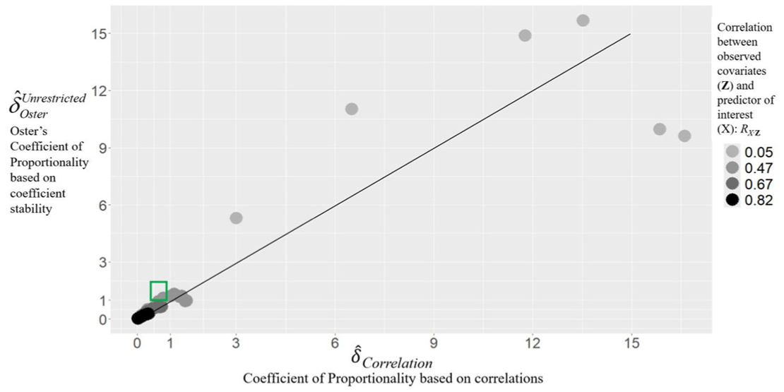
To calculate ${\hat{δ}}_{Oster}^{Unrestricted}$ in the simulated scenarios of Subsection 4.5, we use an unconditional baseline model for which ${\overset{\cdot}{β}}_{1}$ = r_X·Y (σ_Y/σ_X) with ${\overset{\cdot}{R}}^{2} = R_{Y \cdot X}^{2} = r_{X \cdot Y}^{2}$ and $τ_{X} = (1 - R_{X \cdot Z}^{2}) σ_{X}^{2}$ .

Given the values of ${\overset{\cdot}{β}}_{1}$ , ${\overset{\cdot}{R}}^{2}$ , and ${\hat{τ}}_{X}$ , and the other simulated values, we calculated ${\hat{δ}}_{Oster}^{Unrestricted}$ based on Equation 4. This allows us to graphically compare ${\hat{δ}}_{Oster}^{Unrestricted}$ with $\hat{δ}$ _Correlation as in Figure 2. There is high agreement; the two are correlated at .902. But the difference in scales between ${\hat{δ}}_{Oster}^{Unrestricted}$ and $\hat{δ}$ _Correlation is consequential. About 89% (32/36) of the points are above the 45-degree line, implying ${\hat{δ}}_{Oster}^{Unrestricted}$ characterizes the inference as more robust (less conservative) than $\hat{δ}$ _Correlation. Specifically, in the green box, ${\hat{δ}}_{Oster}^{Unrestricted}$ > 1 > $\hat{δ}$ _Correlation (as in the running empirical example). In these scenarios, one would infer from ${\hat{δ}}_{Oster}^{Unrestricted}$ that the inference regarding β₁ is robust using Oster’s (2019, p. 191) threshold of equal selection but not so from $\hat{δ}$ _Correlation.

Figure 2.

Coefficient of Proportionality based on coefficient stability versus correlations.

As in the empirical example, we leverage sampling variability in $\hat{δ}$ _Correlation as a function of r_X·CV to evaluate the difference between ${\hat{δ}}_{Oster}^{Unrestricted}$ and $\hat{δ}$ _Correlation. As reported in Supplemental Table E1, the difference between ${\hat{δ}}_{Oster}^{Unrestricted}$ and $\hat{δ}$ _Correlation is more than twice the standard error of $\hat{δ}$ _Correlation in more than 80% (30/36) of the scenarios (i.e., in 22 scenarios, the difference is more than four times the standard error of $\hat{δ}$ _Correlation); the differences between ${\hat{δ}}_{Oster}^{Unrestricted}$ and $\hat{δ}$ _Correlation are clearly discernable.

Examination of the results in Supplemental Table E1, sorted by $(\frac{{\hat{δ}}_{Oster}^{Unrestricted} - {\hat{δ}}_{Correlation}}{se ({\hat{δ}}_{Correlation})})$ , shows that in general, ${\hat{δ}}_{Oster}^{Unrestricted}$ and $\hat{δ}$ _Correlation are least in agreement when R_max is small. Specifically, the four smallest (negative) values and four largest (positive) differences occur for R_max < .5. Although one important insight from Oster (2019) is that one may not be able to explain all of the variance in Y even if one had access to every conceivable covariate, this logic can be taken too far in calculating ${\hat{δ}}_{Oster}^{Unrestricted}$ , which is highly responsive to small values of R_max.

In an alternative set of scenarios, we added .1 to r_X·Y thereby increasing the change in estimated effect between the baseline (Equation 2a) and intermediate (Equation 2b) models but decreasing the change in R² between the two. In these alternative scenarios, ${\hat{δ}}_{Oster}^{Unrestricted}$ and $\hat{δ}$ _Correlation were correlated only at .60. Thus, the difference between ${\hat{δ}}_{Oster}^{Unrestricted}$ and $\hat{δ}$ _Correlation appears to be due to the extreme responsiveness to coefficient instability relative to change in R² inherent in Oster’s (2019) conceptualization of the COP. Note Se( ${\hat{δ}}_{Oster}^{Unrestricted}$ ) > Se( $\hat{δ}$ _Correlation) because ${\hat{δ}}_{Oster}^{Unrestricted}$ is a function of $\overset{\cdot}{β}$ ₁ and $\overset{\cdot}{R}$ in Equation 2a in addition to the terms in Equation 2b.

7. Revisiting Assumptions for $\hat{δ}$ _Correlation

In this section, we revisit our initial assumptions made in Subsection 4.3 to support a more general application of the COP. Specifically, we evaluate the assumption that the there is only a single unobserved covariate, the unobserved covariate is orthogonal to observed covariates, and that the threshold is specified as absolute without regard to sampling variability.

7.1 Multiple Unobserved Covariates

Oster (2019, pp. 191–192) represented unobserved covariates with a single index, W₂, the predicted value of Y based on all the unobserved covariates. Correspondingly, for initial derivation, we assumed a single unobserved covariate, CV. This allowed us to express the conditions necessary to generate a specified value of ${\overset{⌣}{β}}_{1}$ (β ^# ) and maximum ${\overset{⌣}{R}}^{2}$ (R_max) in model (Equation 2c) in terms of r_X·CV| _Z and r_Y·CV| _Z .

Our initial derivations can be directly extended to multiple unobserved covariates CV by drawing on Knaeble and Dutter (2017) and Knaeble et al.’s (2020) expression for statistical control based on multiple covariates. Applying the result to ${\overset{⌣}{β}}_{1}$ in Equation 2c yields (leveraging the Frisch–Waugh–Lovell decomposition to condition on Z):

{\overset{⌣}{β}}_{1} = \frac{{\hat{σ}}_{Y | Z}}{{\hat{σ}}_{X | Z}} \frac{r_{X \cdot Y | Z} - R_{X \cdot C V | Z} R_{Y \cdot C V | Z} r_{\hat{X} \hat{Y} | Z}}{1 - R_{X \cdot C V | Z}^{2}} = β^{#},

(8)

where $r_{\hat{X} \hat{Y} | Z}$ is the correlation between $\hat{X}$ (the predicted value from regressing X on the elements in CV conditioned on Z) and $\hat{Y}$ (the predicted value from regressing Y on the elements in CV conditioned on Z), with −1 < $r_{\hat{X} \hat{Y} | Z}$ < 1.

Although $r_{\hat{X} \hat{Y} | Z}$ is not observed, we can leverage Equation 8 to show that our expression for $\hat{δ}$ _Correlation in Equation 7 as a function of a single covariate is conservative. For β ^# = 0, the numerator in Equation 8 must equal 0 (assuming ${\hat{σ}}_{Y | Z} > 0$ ) and therefore $R_{X \cdot CV | Z} R_{Y \cdot CV | Z} r_{\hat{X} \hat{Y} | Z} = r_{X \cdot Y | Z}$ . Correspondingly, the minimum value of R_X· _CV|Z R_Y· _CV|Z occurs for $r_{\hat{X} \hat{Y} | Z}$ = 1. When $r_{\hat{X} \hat{Y} | Z}$ = 1 (in which case $R_{X \cdot CV | Z} R_{Y \cdot CV | Z} = r_{X \cdot Y | Z}$ ), the regression weights using the elements in CV to predict X are proportional to those when predicting Y. As a result, R_X· _CV|Z R_Y· _CV|Z can be represented by a single CV* based on the predicted value of X or Y. Equation 8 can then be rewritten replacing R_X· _CV|Z R_Y· _CV|Z with r_X·CV* _|Z r_Y·CV* _|Z . Furthermore, for β ^# = 0, r_Y·CV* _|Z is completely determined by R_max and R_Y· _Z (see Subsection 5.2). As a result, for $r_{\hat{X} \hat{Y} | Z} < 1$ , r_X·CV* _|Z would have to be greater than R_X· _CV|Z to satisfy Equation 8, making $\hat{δ}$ _Correlation larger. Therefore, for β ^# = 0 assuming a single CV represented by CV* is conservative in the sense of producing a small value of $\hat{δ}$ _Correlation, protecting a null hypothesis of zero effect.

For β ^# < 0 (implying a sign change in the estimate of β₁ from Equations 2b to 2c for r_X·Y| _Z > 0), solving Equation 8 for $R_{X \cdot CV | Z}$ yields

R_{X \cdot CV | Z} = \frac{R_{Y \cdot CV | Z} r_{\hat{X} \hat{Y} | Z} \pm \sqrt{4 {(β^{#} \frac{{\hat{σ}}_{X | Z}}{{\hat{σ}}_{Y | Z}})}^{2} - 4 β^{#} \frac{{\hat{σ}}_{X | Z}}{{\hat{σ}}_{Y | Z}} r_{X \cdot Y | Z} + {(R_{Y \cdot CV | Z} r_{\hat{X} \hat{Y} | Z})}^{2}}}{2 β^{#} \frac{{\hat{σ}}_{X | Z}}{{\hat{σ}}_{Y | Z}}} .

(9)

Note that $R_{X \cdot CV | Z}$ is monotonic and decreasing in $r_{\hat{X} \hat{Y} | Z}$ for β ^# < 0. Therefore, the minimum R_X· _CV|Z for flipping the sign of ${\hat{β}}_{1}$ also occurs for $r_{\hat{X} \hat{Y} | Z}$ = 1.^11,12 The result can be extended to the assumption of non-orthogonality in the next subsection because Knaeble and Dutter’s (2017) expression applies to the numerator for the partial correlation in Supplemental Appendix H (Equation H1).

7.2 Unobserved Covariate is Not Orthogonal to Observed Covariates

Oster (2019, p. 192) assumed the unobserved covariate (W₂) is orthogonal to the observed covariates (W₁). In our notation, this implies R_CV· _Z = 0 (for similar assumptions, see Altonji et al., 2005, p. 169; Cinelli & Hazlett, 2020, p. 53; Frank, 2000, p. 165; Ichino et al., 2008, p. 316). The assumption that R_CV· _Z = 0 is necessary to obtain r_X _·CV from r_X _·CV _| _Z and therefore $\hat{δ}$ _Correlation in Equation 7.

In Supplemental Appendix H, we show for a single observed covariate the assumption r_CV·Z = 0 is always conservative (in the sense of minimizing $\hat{δ}$ _Correlation) for $\hat{δ}$ _Correlation < 1. For $\hat{δ}$ _Correlation > 1, the results in Supplemental Appendix H also show that r_CV·Z = 0 is conservative except in the extreme of our simulated scenarios (reported in Supplemental Appendix E) in which r_X·Z < .05 (the observed covariate explains a small amount of variation in X) or r_CV·Z > .92 (observed covariate essentially subsumes the unobserved covariate). Thus, assuming r_CV _·Z = 0 will typically lead to a conservative interpretation of the inference, in the sense of making it more difficult to overturn the null hypothesis of no effect. In Supplemental Appendix E, we also report Max(r_CV·Z), the maximum value of r_CV _·Z for which $\hat{δ}$ _Correlation is a minimum, and thus conservative. The result can be adapted for multiple observed covariates via Subsection 7.1.

7.3 Threshold Based on Statistical Significance, $\hat{δ}$ _Statsig

Although Equation 7 is expressed for any specified threshold β ^# , separate expressions are necessary to calculate the conditions necessary to nullify a statistical inference (e.g., associated with p < .05) regarding β₁. This is because statistical significance is typically a function of the standard error for ${\overset{⌣}{β}}_{1}$ which would change with the inclusion of omitted covariates. To develop an expression based on statistical significance, in Supplemental Appendix J (including application to the empirical example and R code) we define and solve two equations for $R^{2}$ = R_max and r_X·Y| _Z = r_critical (the value of a partial correlation associated with p = .05) for the two unknowns r_X·CV and r_Y·CV, leveraging the fact that the p-value for a partial correlation equals that for the corresponding regression coefficient (Cohen & Cohen, 1983). Ultimately, this generates an expression for $\hat{δ}$ _Statsig that accounts for sampling variability, one of the most commonly used thresholds for inference (Frank et al., 2023).¹³

We apply the result in Supplemental Appendix J to the inference regarding the effect of Low birthweight and preterm on IQ. For Oster’s (2019) specified R_max = .61 and given the other quantities reported by Oster, the partial correlations of r_X·CV| _Z = .0195 and r_Y·CV| _Z = .6928 would generate ${\overset{⌣}{β}}_{1} = . 0714$ , $Se ({\tilde{β}}_{1}) = . 0364$ , with $t = \frac{. 0714}{. 0364} = 1.9608$ associated with p = .05 for df = 6,165. Concurrently, r_X·CV| _Z = .0195 and r_Y·CV| _Z = .6928 generate $R_{Y \cdot XCV | Z}^{2} = . 69269^{2} = . 4805$ corresponding to $R_{Y \cdot XCV Z}^{2} = R_{\max} = . 61$ as in Oster’s specification (see Section 5 and Supplemental Appendix E). Note that the standard error of .0364 for this calculation is smaller than the standard error of 0.050 Oster reported for the observed data. In this sense, the expressions in Supplemental Appendix J account for how the standard error would change if unobserved covariates were added to the model. To calculate the corresponding $\hat{δ}$ _Statsig, we first calculate $r_{X \cdot CV} = \sqrt{1 - R_{X \cdot Z}^{2}} r_{X \cdot CV | Z} = \sqrt{1 - {. 078}^{2}} 0.019514 = 0.019455$ (drawing on Supplemental Appendix B, with extra digits to dif-ferentiate r_X·CV from r_X·CV| _Z ). Then for R_X· _Z = .078, ${\hat{δ}}_{Statsig} = \frac{r_{X \cdot CV}}{R_{X \cdot Z}} = \frac{0.01945524}{. 078} = . 249 .$ Because the threshold for rejecting a null hypothesis of zero effect as greater than zero, $\hat{δ}$ _Statsig of .249 required to reduce the estimated effect below the threshold for statistical significance is less than $\hat{δ}$ _Correlation of .583 required to reduce the effect to zero. That is, $\hat{δ}$ _Statsig will typically be more conservative (smaller) than $\hat{δ}$ _Correlation.

8. Discussion

Beginning with the effects of smoking on lung cancer (Cornfield et al., 1959), sensitivity analyses have shaped debates about causal inferences that can inform policy or practice. In this article, we contributed to the development of the COP which expresses sensitivity in terms of how strong selection on unobserved covariates must be relative to that on observed covariates to nullify an inference (Altonji et al., 2005). Specifically, we have built directly on Oster’s (2019) contributions to the COP in specifying a maximum variance explained if all conceivable covariates were included in a linear model. But we have extended Oster’s application of the COP by reconceptualizing it within a correlational framework. Thus, we wrote, “the correlation between an unobserved covariate and Low birthweight and preterm [r_X·CV] would have to be about 58% that of the very modest multiple correlation associated with the observed covariates (R_X· _Z = .078) to nullify the estimated effect of Low birthweight and preterm on IQ.” The second component of confounding, the relationship of the unobserved covariate to the outcome, is then expressed through a separate correlation (r_Y·CV) that generates a final specified R² (e.g., R²=.61 in the empirical example). Importantly, we showed how the dual components of confounding can then be incorporated through the product, r_X·CVr_Y·CV, defining the impact of a confounding variable (Frank, 2000).

Our reconceptualization of the COP addresses the critiques (e.g., Cinelli & Hazlett, 2020; Diegert et al., 2022; Masten & Poirier, 2022) of Oster (2019) because it is expressed in terms of scale-free correlations and establishes a continuous monotonic relationship between the COP and the estimated effect of the focal predictor. Furthermore, because our COP is rooted in static correlations, our expressions do not depend on an analyst’s specification of a baseline model, are adapted to a threshold for inference based on statistical significance, and can be directly calculated from conventionally reported quantities (e.g., estimated effect, standard error). Furthermore, the assumptions we have made (there is a single unobserved covariate; the unobserved covariates are uncorrelated with the observed covariates) are conservative in terms of protecting the null hypothesis. Finally, using the Konfound package in Stata or R (or the R-shiny app: https://konfound-project.shinyapps.io/konfound-it/), our COP index can be easily applied and intuitively interpreted for most published studies in the social sciences.

8.1 Recommended Practices

8.1.1 Carefully Examine Extent of Selection on Observed Covariates

A by-product of our conceptualization of the COP in terms of correlations is a preliminary calculation of the multiple correlation between the focal predictor and observed covariates (R_X· _Z ). Although covariates can gain impact strength through their relationship to the outcome (Frank, 2000), a small value of R_X· _Z partly undermines the claim that strong covariates were already accounted for and therefore conservatively represent selection on unobserved covariates (e.g., Altonji et al., 2005, pp. 176–177; Oster, 2019, pp. 195–196). The value of R_X· _Z = .078 in the empirical example suggests modest selection on the observed covariates at best. Because R_X· _Z appears in the denominator of our COP in Equation 7, we especially caution against over-interpretation of the COP when R_X· _Z < .05 (and $R_{X \cdot Z}^{2} \leq . 0025$ ). In such cases, one might simply report the correlations associated with the unobserved covariate necessary to produce the specified estimated effect and R² without expressing as a ratio to the limited selection on observed covariates.

8.1.2 Consider a Minimum Value of the Maximum R²

One of Oster’s (2019) key contributions is to consider a limit on the explanatory power of a model even if all conceivable covariates were observed and included. In deriving our expression for $\hat{δ}$ _Correlation, we adopted Oster’s (2019) emphasis on realistic expectations for variance explained in terms of $R_{Y \cdot X Z CV}^{2}$ or R_max. Specifically, Oster (2019, p. 201) established a guideline based on the finding that most (97%) inferences from the randomized studies analyzed would have been sustained for $R_{\max} = 1.3 R_{Y \cdot X Z}^{2}$ , the variance explained in the outcome by the focal predictor (X) and the observed covariates (Z). While Oster’s logic and empirical validation are sound, we note that small values of $R_{Y \cdot X Z}^{2}$ could generate unrealistically small values of R_max, leading the robustness of the inference to be overstated (the smaller the value of R_max, the larger the COP indicating a more robust inference). As a guideline, one might consider an absolute minimum R_max of .15, noting that in our simulations ${\hat{δ}}_{Oster}^{Unrestricted}$ performed poorest for R_max < .15. Moreover, it seems reasonable that one should be able to explain at least 15% of the variation in an outcome if all conceivable covariates could be observed and included in a model.

8.1.3 Specification of the Baseline Model

Oster proved the consistency of ${\hat{δ}}_{Oster}^{Unrestricted}$ using null baseline models including no covariates as in Equation 2a. The proof applies to ${\hat{δ}}_{Oster}^{Unrestricted}$ from baseline models that include covariates only if changes in estimated effects and R² when observed covariates are added to a non-null baseline model are proportional to changes relative to a null baseline model (see Section 2.1). This seems unlikely and an added strong assumption to evaluate.

Opportunity to exploit the baseline model is greater for the COP index than for conventional model specifications because it is not clear what should be included in the baseline model. Oster (2019) did not include baseline covariates in the derivation of the COP but included what some may consider essential covariates in baseline models in empirical examples. In the running empirical example in this article, choosing an unconditional baseline model produced ${\hat{δ}}_{Oster}^{Unrestricted}$ = .487 versus ${\hat{δ}}_{Oster}^{Unrestricted}$ = 1.37 using a baseline model with two covariates (mother age and child female); the choice of baseline model had a marked effect on the interpretation of the robustness of the inference. In applications of Oster’s COP, Paredes (2022, footnote 41) controlled for gender and an indicator for coeducational schools at baseline; Edmunds et al. (2024, Supplemental Materials) cited Altoni et al. (2005) to include only “essential or parsimonious” controls at baseline, but Marcotte (2019, Table 2 column 4) controlled for a more extensive set of covariates. Redding and Grissom (2021) included fixed effects for students, although Oster (2019) did not. Because the different specifications can affect the stability of the estimated focal effect as well as the R² (e.g., fixed effects can dramatically increase R²), the direction and magnitude of bias in the estimation of δ_Oster based on these choices is unclear.

8.1.4 Interpretation of the COP

In general, we avoid specific cut-offs for sensitivity indices (Frank et al., 2023; Frank et al., 2025) because the indices are intended to inform dialog regarding the strength of evidence relative to study design and controls. If an absolute threshold were pre-specified (e.g., $\hat{δ}$ _Correlation > 1), a COP value exceeding that threshold could preempt dialog even for studies with weak designs (e.g., studies in which observed covariates are poorly theorized, defined, or measured). Note that unlike other indices, the COP already has the advantage of being defined relative to a benchmark of observed covariates, facilitating an intuitive interpretation based on existing knowledge of a phenomenon. We do also encourage interpreters of inferences to carefully consider the threshold they choose for making an inference, noting that using statistical significance as a threshold will typically be more conservative in terms of protecting the null hypothesis than using a threshold of zero.

9. Conclusion

Even if one follows all recommended practices and uses a baseline model with no covariates, other critiques of Oster (2019) still apply. Cinelli and Hazlett’s critique based on the scaling of δ_Oster and Masten and Poirier’s (2022) critique based on the non-monotonic and discontinuous relationship between ${\hat{δ}}_{Oster}^{Unrestricted}$ and the corresponding estimated effect are difficult to resolve within Oster’s framework. Because the correlational framework is not vulnerable to the same critiques, can correspond with the two stage regression data generation, does not depend on the specification of the baseline model, and is expressed in terms of the OLS calculations conventionally applied to model (Equation 2c), it is difficult for us to imagine a scenario in which Oster’s ${\hat{δ}}_{Oster}^{Unrestricted}$ would be preferred to $\hat{δ}$ _Correlation as presented here.

Ultimately, like Cornfield et al. (1959), our intent is to inform causal inferences from nonexperimental studies. But we emphasize sensitivity analyses do not, in and of themselves, establish the quality of a model or change an inference. Sensitivity analyses should only be applied after one has maximally leveraged the data and design to estimate the best model possible. What sensitivity analyses can then do is formalize and quantify the hypothetical conditions necessary to nullify an estimated effect to inform debate and corresponding policy based on the strength of evidence. Thus, we re-express the COP based on selection into the treatment in terms of correlations associated with observed and unobserved covariates to make it accessible to as broad a set of stakeholders as possible.

Supplemental Material

sj-pdf-1-jeb-10.3102_10769986261422704 – Supplemental material for Quantifying Sensitivity to Selection on Unobserved Covariates: Recasting the Coefficient of Proportionality Within a Correlational Framework

Supplemental material, sj-pdf-1-jeb-10.3102_10769986261422704 for Quantifying Sensitivity to Selection on Unobserved Covariates: Recasting the Coefficient of Proportionality Within a Correlational Framework by Kenneth A. Frank, Qinyun Lin, Spiro Maroulis, Shimeng Dai, Jihoon Choi, Nicole Jess, Hung-Chang Lin, Yuqing Liu, Sarah Maestrales, Ellen Searle and Jordan Tait in Journal of Educational and Behavioral Statistics

Footnotes

Acknowledgements

The authors acknowledge Brian Knaeble for his thoughtful comments on earlier drafts of this manuscript.

Authors’ Note

This article was presented on August 6, 2025 at the Joint Statistical Meetings, Nashville TN.

Declaration of Conflicting Interests

The authors declared no potential conflicts of interest with respect to the research, authorship, and/or publication of this article.

Funding

The authors disclosed receipt of the following financial support for the research, authorship, and/or publication of this article: This work was supported by U.S. Department of Education Institute for Education Sciences through R305D220022 to Michigan State University. The opinions expressed are those of the authors and do not represent views of the Institute for education Sciences or the U.S. Department of Education.

ORCID iD

Kenneth A. Frank

Supplemental Material

Supplemental material for this article is available online.

Notes

Authors

KENNETH A. FRANK is MSU Research Foundation Distinguished Professor of Sociometrics at Michigan State University. His methodological interests in sensitivity analysis (), causal inference, and social network analysis are driven by his substantive interests in how people draw on their networks to make collective decisions (in organizations and communities).

QINYUN LIN is a Senior Lecturer in Health Science Statistics at the School of Public Health and Community Medicine, University of Gothenburg, Sweden. Her research focuses on causal inference, spatial epidemiology, and sensitivity analysis, with applications to health and educational inequities and the social and contextual factors shaping population outcomes.

SPIRO MAROULIS is Professor and Director of the Martin School of Public Policy and Administration at the University of Kentucky. He is a computational social scientist with a particular focus on public policy and management, innovation, social networks, and causal inference.

SHIMENG DAI is a research associate and project manager at Michigan State University. She received her PhD in Measurement and Quantitative Methods from Michigan State University. Her research focuses on computational social science, STEM education, randomized controlled trials, social network analysis, and natural language processing.

JIHOON CHOI is a PhD student in the Measurement and Quantitative Methods program at Michigan State University. His research interests are in causal inference, with a methodological focus on sensitivity analysis for observational studies and empirical applications to postsecondary educational effectiveness.

NICOLE JESS is a Statistician at Michigan Fitness Foundation, where she conducts program evaluation and research in public health and community settings. She specializes in survey development, latent variable modeling, and quasi-experimental designs, with a focus on supporting evidence-based decision making.

HUNG-CHANG LIN recently received his PhD in Strategic Management from Michigan State University. His research examines the role of language and emotion in markets, particularly investor evaluations of executive communication, with broader methodological interests in natural language processing.

YUQING LIU is a postdoctoral researcher on the Urban-Rural Dialogue project in the Department of Community Sustainability at Michigan State University. Her research includes survey development, program evaluation, and social network analysis of dialogues about urban-rural identities, aiming to improve identity awareness, relationships across differences, bias interruption, and equity-oriented action

SARAH MAESTRALES, Ph.D. (Michigan State University), consults with EdTech startups and educational organizations on AI integration, data workflows, and evaluation practices. Her current work examines how statistical modeling and measurement methods can be used to improve the efficiency, evaluation, and implementation of GenAI systems in educational and applied research settings.

ELLEN SEARLE has a Master’s in Psychology from Michigan State University and is currently pursuing a master’s in data science from the University of Pittsburgh for training that can be applied across the social sciences as well as sport.

JORDAN TAIT (PhD Michigan State University) is an Assistant Teaching Professor in the Information Systems and Analytics Department in the Farmer School of Business at Miami University Oxford, Ohio. In this role, he coordinates Business Statistics. His research interests include sensitivity analysis, social network analysis and students’ self-efficacy.

References

Alberg

A. J.

Shopland

D. R.

Cummings

K. M.

(2014). The 2014 Surgeon General’s report: Commemorating the 50th Anniversary of the 1964 Report of the Advisory Committee to the US Surgeon General and updating the evidence on the health consequences of cigarette smoking. American Journal of Epidemiology, 179(4), 403–412.

Altonji

J. G.

Elder

T. E.

Taber

C. R.

(2005). Selection on observed and unobserved variables: Assessing the effectiveness of Catholic schools. Journal of Political Economy, 113(1), 151–184.

Barnow

B. S.

Cain

G. G.

Goldberger

A. S.

(1980). Issues in the analysis of selectivity bias (Vol. 4). University of Wisconsin, Inst. for Research on Poverty.

Basu

(2023). A critical assessment of a popular econometric method for sensitivity analysis. Available at SSRN 4540836.

Berridge

(2006). The policy response to the smoking and lung cancer connection in the 1950s and 1960s. The Historical Journal, 49(4), 1185–1209.

Bonett

D. G.

(2008). Meta-analytic interval estimation for bivariate correlations. Psychological Methods, 13(3), 173–181. https://doi.org/10.1037/a0012868

Breslau

DelDotto

J. E.

Brown

G. G.

Kumar

Ezhuthachan

Hufnagle

K. G.

Peterson

E. L.

(1994). A gradient relationship between low birth weight and IQ at age 6 years. Archives of Pediatrics & Adolescent Medicine, 148(4), 377–383.

Carnegie

N. B.

Harada

Hill

J. L.

(2016). Assessing sensitivity to unmeasured confounding using a simulated potential confounder. Journal of Research on Educational Effectiveness, 9(3), 395–420.

Cinelli

Hazlett

(2020). Making sense of sensitivity: Extending omitted variable bias. Journal of the Royal Statistical Society: Series B, 82(1), 39–67.

10.

Cohen

(1983). Applied multiple regression. Correlation Analysis for the Behavioral Sciences. Lawrence Erlbaum.

11.

Cornfield

Haenszel

Hammond

E. C.

Lilienfeld

A. M.

Shimkin

M. B.

Wynder

E. L.

(1959). Smoking and lung cancer: Recent evidence and a discussion of some questions. Journal of the National Cancer Institute, 22(1), 173–203.

12.

Diegert

Masten

M. A.

Poirier

(2022). Assessing omitted variable bias when the controls are endogenous. arXiv. arXiv preprint arXiv:2206.02303.

13.

Edmunds

J. A.

Unlu

Furey

Glennie

Arshavsky

(2020). What happens when you combine high school and college? The impact of the early college model on postsecondary performance and completion. Educational Evaluation and Policy Analysis, 42(2), 257–278.

14.

Edmunds

J. A.

Unlu

Phillips

Mulhern

Hutchins

B. C.

(2024). CTE-focused dual enrollment: Participation and outcomes. Education Finance and Policy, 19(4), 612–633.

15.

Fisher

R. A.

(1958). Lung cancer and cigarettes? Nature, 182(4628), 108.

16.

Frank

K. A.

(2000). Impact of a confounding variable on the inference of a regression coefficient. Sociological Methods and Research, 29(2), 147–194.

17.

Frank

K. A.

Lin

Maroulis

S. J.

(2025). Causal inferences from observational studies in education policy: Towards pragmatic social science. In Cohen-Vogel

Scott

Youngs

(Eds.), Handbook on education policy research (pp. 479–510). The American Educational Research Association.

18.

Frank

K. A.

Lin

Maroulis

Mueller

A. S.

Rosenberg

J. M.

Hayter

C. S.

Mahmoud

R. A.

Kolak

Dietz

Zhang

(2021). Hypothetical case replacement can be used to quantify the robustness of trial results. Journal of Clinical Epidemiology, 134, 150–159.

19.

Frank

K. A.

Lin

Maroulis

S. J.

Mueller

(2023). Quantifying the robustness of causal inferences: Sensitivity analysis for pragmatic social science. Social Science Research, 110, 102815.

20.

Frank

K. A.

Maroulis

Duong

Kelcey

(2013). What would it take to change an inference?: Using Rubin’s causal model to interpret the robustness of causal inferences. Education, Evaluation and Policy Analysis, 35, 437–460.

21.

Franks

D’Amour

Feller

(2019). Flexible sensitivity analysis for observational studies without observable implications. Journal of the American Statistical Association, 115, 1730–1746.

22.

Frisch

Waugh

F. V.

(1933). Partial time regressions as compared with individual trends. Econometrica: Journal of the Econometric Society, 1, 387–401.

23.

Gastwirth

J. L.

Krieger

A. M.

Rosenbaum

P. R.

(1998). Dual and simultaneous sensitivity analysis for matched pairs. Biometrika, 85(4), 907–920.

24.

Gross

R. T.

Spiker

Haynes

C. W.

(1997). Helping low birth weight, premature babies: The infant health and development program. Stanford University Press.

25.

Hirano

Imbens

G. W.

(2001). Estimation of causal effects using propensity score weighting: An application to data on right heart catheterization. Health Services and Outcomes Research Methodology, 2(3), 259–278.

26.

Holland

P. W.

(1986). Statistics and causal inference. Journal of the American Statistical Association, 81(396), 945–960.

27.

Hong

Qin

Yang

(2018). Weighting-based sensitivity analysis in causal mediation studies. Journal of Educational and Behavioral Statistics, 43(1), 32–56.

28.

Hong

Yang

Qin

(2021). Did you conduct a sensitivity analysis? A new weighting-based approach for evaluations of the average treatment effect for the treated. Journal of the Royal Statistical Society: Series A (Statistics in Society), 184(1), 227–254.

29.

Hosman

C. A.

Hansen

B. B.

Holland

P. W.

(2010). The sensitivity of linear regression coefficients’ confidence limits to the omission of a confounder. The Annals of Applied Statistics, 4(2), 849–870.

30.

Hsu

J. Y.

Small

D. S.

(2013). Calibrating sensitivity analyses to observed covariates in observational studies. Biometrics, 69(4), 803–811.

31.

Ichino

Mealli

Nannicini

(2008). From temporary help jobs to permanent employment: What can we learn from matching estimators and their sensitivity? Journal of Applied Econometrics, 23(3), 305–327.

32.

Imai

Keele

Yamamoto

(2010). Identification, inference and sensitivity analysis for causal mediation effects. Statistical Science, 25(1), 51–71.

33.

Imbens

(2003). Sensitivity to exogeneity assumptions in program evaluation. American Economic Review, 93(2), 126–132.

34.

Johnson

R. A.

Wichern

D. W.

(2002). Applied multivariate statistical analysis. Prentice Hall.

35.

Knaeble

Dutter

(2017). Reversals of least-square estimates and model-invariant estimation for directions of unique effects. The American Statistician, 71(2), 97–105.

36.

Knaeble

Osting

Abramson

M. A.

(2020). Regression analysis of unmeasured confounding. Epidemiologic Methods, 9(1), 20190028.

37.

Kramer

M. S.

(1987). Intrauterine growth and gestational duration determinants. Pediatrics, 80(4), 502–511.

38.

Lin

D. Y.

Psaty

B. M.

Kronmal

R. A.

(1998). Assessing the sensitivity of regression results to unmeasured confounders in observational studies. Biometrics, 54, 948–963.

39.

Lonati

Wulff

J. N.

(2024). Hic Sunt Dracones: On the risks of comparing the ITCV with control variable correlations. Journal of Management, 52, 0149206324 1293126.

40.

Lovell

M. C.

(1963). Seasonal adjustment of economic time series and multiple regression analysis. Journal of the American Statistical Association, 58(304), 993–1010.

41.

Marcotte

D. E.

(2019). The returns to education at community colleges: New evidence from the Education Longitudinal Survey. Education Finance and Policy, 14(4), 523–547.

42.

Masten

M. A.

Poirier

(2022). The effect of omitted variables on the sign of regression coefficients. arXiv. arXiv preprint arXiv:2208.00552.

43.

Mauro

(1990). Understanding LOVE (left out variables error): A method for estimating the effects of omitted variables. Psychological Bulletin, 108(2), 314.

44.

Middleton

J. A.

Scott

M. A.

Diakow

Hill

J. L.

(2016). Bias amplification and bias unmasking. Political Analysis, 24(3), 307–323.

45.

National Research Council. (2000). From neurons to neighborhoods: The science of early childhood development. National Academies Press.

46.

Oster

(2019). Unobservable selection and coefficient stability: Theory and evidence. Journal of Business & Economic Statistics, 37(2), 187–204.

47.

Paredes

(2022). Mixed but not scrambled: Gender gaps in coed schools with single-sex classrooms. Journal of Research on Educational Effectiveness, 15(2), 330–366.

48.

Park

Esterling

K. M.

(2021). Sensitivity analysis for pretreatment confounding with multiple mediators. Journal of Educational and Behavioral Statistics, 46(1), 85–108.

49.

Pearl

(2009). Causality. Cambridge University Press.

50.

Redding

Grissom

J. A.

(2021). Do students in gifted programs perform better? Linking gifted program participation to achievement and nonachievement outcomes. Educational Evaluation and Policy Analysis, 43, 01623737211008919.

51.

Rice

J. A.

(2006). Mathematical statistics and data analysis. Cengage Learning.

52.

Robins

J. M.

Rotnitzky

Scharfstein

D. O.

(2000). Sensitivity analysis for selection bias and unmeasured confounding in missing data and causal inference models. In M. E. Halloran & D. A. Berry (Eds.), Statistical models in epidemiology, the environment, and clinical trials (pp. 1–94). Springer.

53.

Rosenbaum

P. R.

(2002). Observational studies. Springer.

54.

Rosenbaum

P. R.

(1986). Dropping out of high school in the United States: An observational study. Journal of Educational Statistics, 11(3), 207–224.

55.

Rosenbaum

P. R.

(2005). Sensitivity analysis in observational studies. Encyclopedia of Statistics in Behavioral Science, 4, 1809–1814.

56.

Rosenbaum

P. R.

Rubin

D. B.

(1983). Assessing sensitivity to an unobserved binary covariate in an observational study with binary outcome. Journal of the Royal Statistical Society: Series B (Methodological), 45(2), 212–218.

57.

Rosseel

(2012). lavaan: An R package for structural equation modeling. Journal of Statistical Software, 48, 1–36.

58.

Strawson

P. F.

(2008). Freedom and resentment and other essays. Routledge.

59.

U.S. Department of Health, Education, and Welfare. (1964). Smoking and Health: Report of the Advisory Committee to the Surgeon General of the Public Health Service. Washington, DC: US Department of Health, Education, and Welfare, Public Health Service (Public Health Service Publication No. 1103).

60.

US Public Health Service. Office of the Surgeon General, United States. Office on Smoking, Center for Chronic Disease Prevention, & Health Promotion (US). Office on Smoking. (1989). Reducing the Health Consequences of Smoking: 25 Years of Progress: A Report of the Surgeon General, Centers for Disease Control. Rockville, Maryland.

61.

VanderWeele

T. J.

Ding

(2017). Sensitivity analysis in observational research: introducing the E-value. Annals of Internal Medicine, 167(4), 268–274.

62.

Veitch

Zaveri

(2020). Sense and sensitivity analysis: Simple post-hoc analysis of bias due to unobserved confounding. Advances in Neural Information Processing Systems, 33, 10999–11009.

63.

Zachrisson

H. D.

Dearing

Borgen

N. T.

Sandsør

A. M. J.

Karoly

L. A.

(2023). Universal early childhood education and care for toddlers and achievement outcomes in middle childhood. Journal of Research on Educational Effectiveness, 17, 1–29.

Supplementary Material

Please find the following supplemental material available below.

For Open Access articles published under a Creative Commons License, all supplemental material carries the same license as the article it is associated with.

For non-Open Access articles published, all supplemental material carries a non-exclusive license, and permission requests for re-use of supplemental material or any part of supplemental material shall be sent directly to the copyright owner as specified in the copyright notice associated with the article.

1.64 MB

0.00 MB

Quantifying Sensitivity to Selection on Unobserved Covariates: Recasting the Coefficient of Proportionality Within a Correlational Framework

Abstract

Keywords

1. Introduction

2. Oster’s COP: δoster

2.1 Definition of δoster

2.2 Estimation of δoster

2.3 Example Application: Effect of Low Birthweight and Preterm on Infant IQ

3. Critiques of Oster’s COP (δOster)

4. Recasting the COP in a Correlational Framework: δCorrelation

4.1 Notation

4.2 Definition of δCorrelation

4.3 Initial Assumptions for Estimation

4.4 Estimation of δCorrelation

4.5 Verification of δ ^ Correlation Through Simulation

5. Application of δCorrelation: Estimated Effect of Low Birthweight and Preterm Status on IQ

5.1 Calculation of δ ^ Correlation

5.2 Recovery of rX·CV and rY·CV Defining the Impact of the Confounding Variable

6. Differences Between δ ^ Oster Unrestricted and δ ^ Correlation

6.1 Example of Estimated Effect of Preterm and Low Birthweight on IQ

6.2 Comparison of δ ^ Oster Unrestricted and δ ^ Correlation Through Simulation

7. Revisiting Assumptions for δ ^ Correlation

7.1 Multiple Unobserved Covariates

7.2 Unobserved Covariate is Not Orthogonal to Observed Covariates

7.3 Threshold Based on Statistical Significance, δ ^ Statsig

8. Discussion

8.1 Recommended Practices

8.1.1 Carefully Examine Extent of Selection on Observed Covariates

8.1.2 Consider a Minimum Value of the Maximum R2

8.1.3 Specification of the Baseline Model

8.1.4 Interpretation of the COP

9. Conclusion

Supplemental Material

sj-pdf-1-jeb-10.3102_10769986261422704 – Supplemental material for Quantifying Sensitivity to Selection on Unobserved Covariates: Recasting the Coefficient of Proportionality Within a Correlational Framework

Footnotes

Acknowledgements

Authors’ Note

Declaration of Conflicting Interests

Funding

ORCID iD

Supplemental Material

Notes

Authors

References

Supplementary Material

2. Oster’s COP: δ_oster

2.1 Definition of δ_oster

2.2 Estimation of δ_oster

3. Critiques of Oster’s COP (δ_Oster)

4. Recasting the COP in a Correlational Framework: δ_Correlation

4.2 Definition of δ_Correlation

4.4 Estimation of δ_Correlation

4.5 Verification of $\hat{δ}$ _Correlation Through Simulation

5. Application of δ_Correlation: Estimated Effect of Low Birthweight and Preterm Status on IQ

5.1 Calculation of $\hat{δ}$ _Correlation

5.2 Recovery of r_X·CV and r_Y·CV Defining the Impact of the Confounding Variable

6. Differences Between ${\hat{δ}}_{Oster}^{Unrestricted}$ and $\hat{δ}$ _Correlation

6.2 Comparison of ${\hat{δ}}_{Oster}^{Unrestricted}$ and $\hat{δ}$ _Correlation Through Simulation

7. Revisiting Assumptions for $\hat{δ}$ _Correlation

7.3 Threshold Based on Statistical Significance, $\hat{δ}$ _Statsig

8.1.2 Consider a Minimum Value of the Maximum R²