Transferring experiences in k-nearest neighbors based multiagent reinforcement learning: an application to traffic signal control

Abstract

The increasing demand for mobility in our society poses various challenges to traffic engineering, computer science in general, and artificial intelligence in particular. Increasing the capacity of road networks is not always possible, thus a more efficient use of the available transportation infrastructure is required. Another issue is that many problems in traffic management and control are inherently decentralized and/or require adaptation to the traffic situation. Hence, there is a close relationship to multiagent reinforcement learning. However, using reinforcement learning poses the challenge that the state space is normally large and continuous, thus it is necessary to find appropriate schemes to deal with discretization of the state space. To address these issues, a multiagent system with agents learning independently via a learning algorithm was proposed, which is based on estimating Q-values from k-nearest neighbors. In the present paper, we extend this approach and include transfer of experiences among the agents, especially when an agent does not have a good set of k experiences. We deal with traffic signal control, running experiments on a traffic network in which we vary the traffic situation along time, and compare our approach to two baselines (one involving reinforcement learning and one based on fixed times). Our results show that the extended method pays off when an agent returns to an already experienced traffic situation.

Keywords

Traffic signal control multiagent reinforcement learning transfer learning

1. Introduction

Traffic congestion is a well investigated phenomenon in traffic engineering, having various deleterious consequences: air pollution, decrease in speed, delays, opportunity costs, etc. The increase in transportation demand can be met by providing additional capacity. However, this might not be economically or socially attainable or feasible. Thus, optimizing the use of the existing infrastructure is key. One way to accomplish this is by employing control techniques, notably the adaptive control of traffic signals. We stress that optimizing such a controller is not trivial since the problem is very constrained, given that minimum and maximum green times need to be observed, and the control policy needs to be fair to all traffic directions in order to deal with starvation.

Several approaches to adaptive control exist (see, e.g., [22] and the surveys mentioned ahead). Among them, approaches based on reinforcement learning (RL) are gaining popularity. In these approaches, learning agents are normally in charge of controlling the signals at a single intersection, in a decentralized way, i.e., each agent learns independently and without a central agent in charge of all intersections. We remark that for centralized approaches, where there is a single controller in charge of computing optimal actions for the whole set of intersections, deep learning is more popular. However, due to robustness issues (central point of failure, communication failures), it is desirable to avoid centralized solutions. Besides, centralized approaches assume a central entity in charge of the control, which needs to collect all information from all intersections, and needs to determine an action for each controller at the intersections, thus violating the autonomy of the individual controllers. To circumvent this, in this paper we deal with multiple agents (signal controllers) learning independently in a decentralized way.

One important aspect of such learning task is that traffic signal control is a highly non-local phenomenon, i.e., it is affected by actions of other agents. This is what makes multiagent RL much more challenging than single agent RL. Another challenge is the fact that the state space is very large (thus RL algorithms like Q-learning converge more slowly) and continuous (appropriately discretizing continuous states is a difficult problem).

That being said, alternatives to tackle these matters, like function approximation, come with some drawbacks. They make the learned policy harder to comprehend, and generally require that the agents gather a large amount of data to be able to successfully generalize and apply their collected experiences.

To tackle large continuous state spaces in an efficient way, in [11] we have started investigating the use of a method that avoids the usage of function approximation, while also dealing with discretization in a more effective way. For this purpose, a learning algorithm based on k-nearest neighbors (k-NN) [17,18] was used, which estimates the value of a state by calculating a weighted average of the Q-values of the k closest previously visited states. However, given that the agents may not have k good experiences, in the present paper we allow agents to transfer their experiences.

The reader can find details of the proposed method in Section 4, where it is described in a general way, as we believe the framework can be applied to several multiagent RL problems. Then, in Section 5 we discuss how to apply the method to the domain of traffic signal control. Our results are presented and discussed in Section 6. The underlying concepts used in this paper (e.g., on RL and RL-based signal control), as well as the related literature are discussed in Section 2 and Section 3, respectively. A conclusion and a discussion on future research lines appear in Section 7.

2. Background on traffic assignment and reinforcement learning

This section briefly presents underlying concepts on RL and on traffic signal control.

2.1. Reinforcement learning

In RL, an agent learns how to act in an environment interacting and receiving a feedback signal (reward) that measures how its action has affected the environment. The agent does not a priori know how its actions affect the environment, hence it has to learn this by trial and error (in an exploration phase). However, the agent should not only explore; in order to maximize the rewards of its action, it also has to exploit the gained knowledge. Thus, there must be an exploration-exploitation strategy that is to be followed by the agent. One of these strategies is ε-greedy, where an action is randomly chosen (exploration) with a probability ε, or, with probability 1-ε, the best known action is chosen, i.e., the one with the highest value so far (exploitation).

In the exploitation phase, it is assumed that the agent has sensors to determine its current state and can then decide on an action. The reward is then used to update its policy, i.e., a mapping from states to actions. This policy can be generated or computed in several ways.

For the sake of the present discussion, we concentrate on a model-free, off-policy algorithm called Q-learning [30], which estimates so-called Q-values using a table to store the experienced values of performing a given action when in a given state. Hence Q-learning is a tabular method, where the state space and the action space need to be discretized.

In RL, the learning task is usually formulated as a Markov decision process (MDP), that defines the sets of states and actions, a transition function, and a reward function. Since the transition and the reward functions are unknown to the agent, its task is exactly to learn them, or at least a model for them.

In Q-learning, the value of a state $s_{t}$ and action $a_{t}$ at time t is updated based on Eq. (1), where $α \in [0, 1]$ is the learning rate, $γ \in [0, 1]$ is the discount factor, $s_{t + 1}$ is the next state and $r_{t}$ is the reward received when the agent moves from $s_{t}$ to $s_{t + 1}$ after selecting action $a_{t}$ in state $s_{t}$ . $\begin{matrix} (1) & Q (s_{t}, a_{t}) \leftarrow Q (s_{t}, a_{t}) + α (r_{t} + γ max_{a} (Q (s_{t + 1}, a)) - Q (s_{t}, a_{t})) \end{matrix}$

When there are multiple agents interacting in a common environment, the RL task (thus, multiagent RL) is inherently more complex because agents’ actions are highly coupled and agents are trying to adapt to other agents that are also learning. Besides, several convergence guarantees no longer hold. However, in many real-world problems, where the control is decentralized, it might not be possible to avoid a multiagent RL formulation, as for instance the scenario we deal with in the present paper, namely control of traffic signals, whose basic concepts we briefly review in the next section.

Before, we mention that in systems in which learning agents are allowed to communicate, there has been some research on how to improve effectiveness and efficiency by allowing transfer of knowledge among agents in multiagent systems. While there are many ways to consider transfer learning techniques, as well as many dimensions of this task, in the present paper we deal with transfer of experiences. The interested reader is referred to [24,25] for more details on multiagent transfer learning.

2.2. RL-based traffic signal control

Besides safety and other issues, one aim of a traffic signal controller is to decide on a split of green times among the various phases that were designed to deal with geometry and flow issues at an intersection. This can be done in several ways (for more details, please see a textbook such as [22]). In this paper, the controller is given a set of phases and has to decide which one will receive green light.

A phase is defined as a group of non-conflicting movements (e.g., flow in two opposite traffic directions) that can have a green light at the same time without conflict.

In its simplest form, the control is based on fixed times, whose split of the green time among the various phases can be computed based on historical data on traffic flow, if available. The problem with this approach is that it may have difficulties adapting to changes in the traffic demand. This may lead to an increase in the number of stopped vehicles. To mitigate this problem, it is possible to use an adaptive scheme and thus give priority to lanes with longer queues (or other measures of performance). Adaptive approaches based on RL were developed, as we discuss next.

3. Related work

Traffic control techniques stem mainly from the areas of control theory and operations research. See for instance [21,22]. More recently though, techniques from artificial intelligence and multiagent systems have also been employed, especially in connection with RL. RL is used by traffic signals to learn a policy that maps states (usually queues at intersections) to actions. Due to the number of works that employ RL for traffic control, the reader is referred to surveys [9,16,19,31,34].

In any case, these surveys show that there has already been a significant contribution of RL techniques to control of traffic signals. However, issues of scalability and performance remain open, especially if tabular methods are used, as for instance the aforementioned Q-learning. Tabular methods require discretization of the state space. The finer such discretization is, the poorer the computational performance tends to be, since agents need to visit an increasing number of state-action pairs that are associated with the learning task at hand.

Therefore, the remaining of this section discusses alternative ways to tackle these issues, which are discussed in the literature.

A first line of research does use tabular methods, changing the level of discretization of the state space, which leads to different levels of performance of the learning task. In this class, well-known works include [6,8,12,33], among others.

A second class of works avoids using tabular methods such as Q-learning. Rather, they propose the use of function approximation. For instance, [2] uses tile coding. Recently, many studies have used deep neural networks to approximate the Q-function (e.g., DQN [29]). However, non-linear function approximation is known to diverge in multiple cases [7,26]. In order to address these shortcomings, [5] proposed the use of linear function approximation, which has guaranteed convergence and error bounds.

A third research line employs clustering methods together with some kinds of RL-based approach in order to tackle the large or continuous state space. For instance, in [1] a hierarchical multiagent system is used, which has two levels: the physical intersection one and the region level. In the former agents use RL to find the best policy and send local information to an agent at region level. At this level, the locally collected information is used to train a long short-term memory (LSTM) neural network for traffic status prediction. The agents in the above level can control the traffic signals by finding the best joint policy using the predicted traffic information.

Finally, another way to tackle the issues that arise from large and continuous state spaces appeared in [17,18], in which a temporal difference learning algorithm based on k-nearest neighbors was presented. RL approaches based on this technique have been used in different domains, like robot motion control [13] and video streaming [14]. More recently, we have studied the use of this technique also in traffic signal control, with preliminary results presented in [11].

In any case, one needs to stress that a multiagent setting is inherently non-stationary, making the learning task even more challenging.

This paper also deals with transferring of experiences among agents, which is related to transfer learning. Since learning a task and adapting to changes in dynamic environments are usually computationally expensive in real-world applications, one solution is to profit from other agents knowledge. Transfer learning is a method to deal with this. Multiple agent can share their experiences, policy or any other knowledge through learning. The knowledge can be transferred from expert agents or more experienced agents [23]. It can also be advice-based transfer in which human teachers [20,28] or adviser agent [35]. In [10], an expert-free transfer learning was utilized in multi-agent reinforcement learning in which source agent is dynamically selected according to the performance and uncertainty measured using interactions. The readers are referred to [24,25,27] for more details on transfer in reinforcement leaning.

4. Combining and transferring nearest neighbors’ knowledge with Q-learning: General framework

As aforementioned, our approach aims at tackling two challenges. First, in many real world problems, the state space that is associated with an RL task is large and/or continuous. Therefore, the quality of the learning task depends on how the state is discretized.

The second challenge is how to improve the learning task by means of having agents communicating their experiences, so that agents that do not have a number k of good experiences can profit from having them transferred from other agents.

The remaining of this section details how to deal with these two challenges by means of combining Q-learning with k-NN, as well as by transferring experiences.

4.1. Temporal difference learning based on k-nearest neighbors

Essentially, the method estimates the Q-values of the current state by calculating the weighted average of the Q-value estimates of the k nearest states, based on the Euclidean distance. The closer a neighbor state is, the greater the impact its estimated Q-value have on the Q-values of the current state.

Once the Q-values are updated this way, each agent then selects an action based on an exploration strategy such as ε-greedy, transitions to a new state and receives a reward. Subsequently, it calculates a temporal difference (TD) error based on the reward and the expected value of the last and new state, and uses this error to update the Q-value estimates of all the k nearest states that contributed to estimate the Q-values of the previous state.

The next subsections details these procedures.

4.1.1. Estimating Q-values

Each dimension of the state space could be of a different order of magnitude. In order to avoid a bias (towards some of these dimensions) when computing the Euclidean distance between two states, we use normalization, as stated in Eq. (2), where $s_{t}$ is the state observed at time step t, and $s_{m}$ and $s_{M}$ denote the lower and upper bounds of the state space (that is, vectors composed of the smallest and largest possible values for each state dimension, respectively). $\begin{matrix} (2) & \hat{s_{t}} = 2 \cdot (\frac{s_{t} - s_{m}}{s_{M} - s_{m}}) - 1 \end{matrix}$

The agent keeps a record of each visited state and an estimate of the Q-values for each of these states. After normalization, the k nearest previously visited states according to the Euclidean distance are selected, in order to determine the k-nearest neighbors set.

A weight is then calculated for each state in the set, according to Eq. (3), where $w_{i}$ and $d_{i}$ represent the weight of the $i_{th}$ nearest state and the Euclidean distance between $s_{t}$ and the $i_{th}$ nearest state, respectively, and $K$ represents the k-nearest neighbors set. $\begin{matrix} (3) & w_{i} = \frac{1}{1 + d_{i}^{2}}, \forall i \in K \end{matrix}$

The Q-value of a state-action pair is determined by an estimate of the expected value, in which the probabilities of each state in the $K$ set are given by Eq. (4), where $p (i)$ is the probability of the $i_{th}$ nearest state in the $K$ set. $\begin{matrix} (4) & p (i) = \frac{w_{i}}{\sum_{j \in K} w_{j}}, \forall i \in K \end{matrix}$

For each action a, the Q-value of the state-action pair ( $s_{t}$ , a) is then determined according to an estimate of expected value using the probabilities and the current estimates of the Q-values of each state in the k-nearest neighbors set, according to Eq. (5). $\begin{matrix} (5) & Q (s_{t}, a) = \sum_{i \in K} p (i) Q (i, a) \end{matrix}$

This way, the method estimates the Q-values of the current state by calculating the weighted average of the Q-values of the nearest previously visited states.

4.1.2. Action selection and updating Q-values

Having the expected value of each action for the current state $s_{t}$ , an exploration strategy, such as ε-greedy, is used to select an action $a_{t}$ . After taking the selected action, the agent transitions to a new state $s_{t + 1}$ and receives a reward $r_{t}$ . In order for learning to occur, the agent estimates the expected value of taking each possible action in the next state, $s_{t + 1}$ , via the k-NN approach explained in Section 4.1.1 (using Eq. (2), Eq. (3), Eq. (4) and Eq. (5) on $s_{t + 1}$ ), and calculates the TD error δ (which is the basic update rule of a TD learning method, obtained by measuring the difference between the estimated value of a state or a state-action pair, and the improved estimate obtained after gaining more experience), using Eq. (6). $\begin{array}{c} (6) & δ = r_{t} + γ max_{a} (Q (s_{t + 1}, a)) - Q (s_{t}, a_{t}) \\ (7) & Q (i, a_{t}) \leftarrow Q (i, a_{t}) + α δ p (i), \forall i \in K \end{array}$

4.2. Communicating agents transferring experiences

At every time step, each agent observes a new state and tries to select the k experiences (Q-values associated with such new state) that are nearest to this observed state. However, if the distance between any of these experiences and the current state is greater than a distance threshold Δ (a parameter of the model), then the agent requests experiences from other agents. These then select all experiences that are within the distance threshold of the requesting agent’s current state, and then send these experiences to the requesting agent. The requesting agent then recomputes the k nearest experiences, and estimates the Q-values for each action based on the standard k-NN-based algorithm.

4.3. Pseudo-code

Algorithm 1:

Temporal difference learning based on k-nearest neighbors

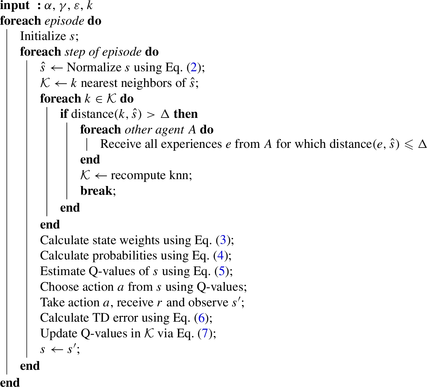
A pseudocode for the overall procedure – combining Q-learning with k-NN and transferring of experiences – is presented in Algorithm 1.

At every time step, the agent observes a state and normalizes it according to Eq. (2). Then, a set $K$ composed of the k nearest experiences to the current state is calculated. The distance between the current state and each experience in $K$ is compared to a distance threshold Δ. If $distance (k, \hat{s}) > Δ$ , then the agent requests experiences from other agents.

Each other agents selects all of the experiences that have a distance to the current state equal to or less than Δ, that is, all experiences e for which $distance (e, \hat{s}) ⩽ Δ$ , and sends these experiences to the requesting agent. Having received these new experiences, the agent then recomputes $K$ , by selecting the k nearest experiences to the current state (considering the agent’s previous experiences and the experiences sent by the other agents). This means that, after the transfer process, the set of $K$ is defined, without further transfers (see the break statement.

Once $K$ is set for that particular state and decision point, the experiences in $K$ are used to determine the weights (Eq. (3)), probabilities (Eq. (4)) and estimate the Q-values of the current state, by using Eq. (5). Having estimated the Q-values, the agent proceeds to select an action, take that action, observe a new state $s^{'}$ and receive a reward r. The agent then calculates the temporal difference error using Eq. (6), and finally updates the Q-values of all the experiences in $K$ using Eq. (7).

5. Application in traffic signal control

The problem of large and continuous state space arises typically in RL-based traffic signal control, where the possible formulations for states may consider queue length, density of vehicles, and also a handful of other features. The reader is referred to [32] for a discussion about popular formulations of the state space for this particular domain.

Next, we discuss the particular formulation of the RL task as used in the present paper, which is a popular one (e.g., [4,5,16]. Before, we introduce the actual traffic network used, in order to refer to it when we discuss how the RL task was formulate.

5.1. Scenario

Fig. 1.

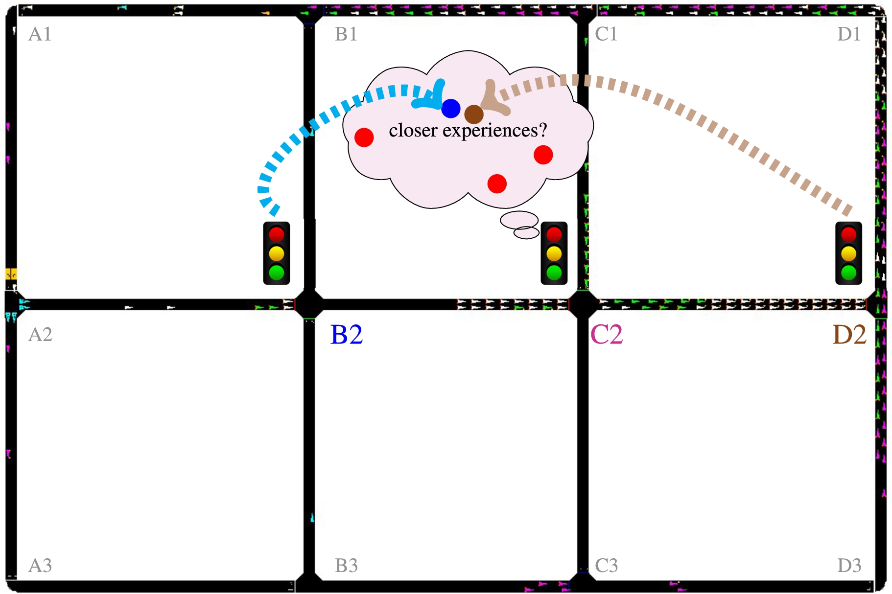
Road network used in the experiments. This figure also depicts a scheme of the communication among the traffic signal control agents (agent C2 lacks experiences and thus request them; agents B2 and D2 send their experiences).

To illustrate the application of our approach, we use the traffic network with 12 intersections depicted in Fig. 1. However, since the links are one-way, not all intersections require a traffic signal controller. This is the case of the four corner intersections, as well as intersections A2, C1, and B3. Other non-signalized intersections are B1 and C3. These two are regulated by a priority mechanism defined in the microscopic simulator used (SUMO), namely all vehicles decelerate before reaching the intersection and SUMO regulates the right of using the intersection. We did this in order to concentrate on the intersections defined by the arterial depicted in the middle of the figure, namely the one that starts at intersection A2 and ends at D2. In this arterial, there are three signalized intersections that are then controlled by a learning agent, namely B2, C2, and D2. Each of these agents learns using the method described in Section 4. More details on SUMO’s priority mechanism can be found at https://sumo.dlr.de/docs/Simulation/Traffic_Lights.html. For an overview on SUMO, see [15].

We also stress that we have created this network with a particular feature in mind: the total number of vehicles is kept constant (except for the first steps, when they are still being inserted at the link B3-C3). This avoids many problems related to the network introduced in [4] and also used in [11], where it was not possible to fully isolate the behavior of the RL approach from SUMO’s mechanism for routing vehicles. In the network depicted in Fig. 1, there is a re-routing device right before intersection A2 that is responsible to re-route each vehicle from time to time. Essentially vehicles keep running in loops, never leaving the simulation. This allows us to control how the trips use the network, which is an important question we deal with here, as described next.

In [4,11] it was shown that the respective methods were able to adapt to change in traffic contexts or simply context. By context we mean that, from time to time, the way trips are distributed over the routes were changed. Note that this does not mean that the number of trips (vehicles) changes but, rather that each trip may use a different route, thus the use of the links, and, hence, of the intersections, differs along time. In the aforementioned papers, the task of setting and controlling the change in contexts faced difficulties because vehicles kept being consumed at their destinations, while new ones were generated, so that at any given time, the number of vehicles kept changing.

In the present paper we decided to have a more stable scheme. We generate a number of trips (200, which, for this network represents almost 50% of overall density, given that its maximum capacity is around 500 vehicles1

The network has 17 one-way links of 150 meters; each vehicle occupies 5 meters when queued.

). Once those 200 vehicles are loaded, they never leave the simulation, being just re-routed to account for changes in context. These changes occur at each 5000 simulation steps, as discussed in Section 5.3, where we show how the various flows of vehicles change along the simulation time.

5.2. Formulation of the RL task

As is often with RL problems, we use a multiagent MDP (MMDP) to formalize the learning task. In the traffic signal control domain, besides the set of agents, we need to define the other sets and functions that compose the MDP. Next, we define the state space, the action space, and the reward function.

Before, we make two remarks. The first is that the discussion ahead considers two kinds of time steps: simulation time and action time. The former corresponds to 1 second of real-world clock, whereas the latter is the time step in which the agent makes a decision about which action to select, given its observed state. In the present paper, one action time step occurs at each five seconds of the real-world clock. This makes sense as signal controllers never make decisions – which could change phases – at each second. All plots depicted in Section 6 refer to the real-world clock.

The second remark refers to classical parameters when controlling traffic signals, namely, the minimum and the maximum time they must remain green. They are referred to as minGreenTime and maxGreenTime, respectively.

5.2.1. State space

At each action time step t, each agent observes a vector $s_{t}$ , which describes the current state of the respective intersection. We use the default state definition in [3], shown in Eq. (8), where $ρ_{1} \in {0, 1}$ and $ρ_{2} \in {0, 1}$ are binary variables that indicate the current active green phase (see Section 2.2 for an explanation on how phases are set). $g \in {0, 1}$ is a binary variable that indicates whether or not the current green phase has been active for more than minGreenTime.

Be L the set of all incoming lanes. The density $Δ_{l} \in [0, 1]$ is defined as the number of vehicles in the incoming lane $l \in L$ divided by the total capacity of the lane. $q_{l} \in [0, 1]$ is defined as the number of queued or stopped vehicles in the incoming lane $l \in L$ divided by the total capacity of the lane. As per default in SUMO, a vehicle is considered to be queued if its speed is below 0.1 m/s. $\begin{matrix} (8) & s_{t} = [ρ_{1}, ρ_{2}, g, Δ_{1}, \dots, Δ_{| L |}, q_{1}, \dots, q_{[L]}] \end{matrix}$

Note that while it is common in the literature that only one feature be used (i.e., either density or queue), here we employ both as this was shown to be more efficient (see [4]).

5.2.2. Action space

Each learning agent chooses a discrete action $a_{t}$ at each action time step t. For our scenario, since all intersections have two incoming links, there are two phases, so each agent has only two actions: keep and change. The former keeps the current green signal active, while the latter switches the current green light to another phase. The agents can only choose keep if the current green phase has been active for less than maxGreenTime, and can only choose change if the current green phase has been active for more than minGreenTime.

5.2.3. Reward function

Let ${n_{queued}}_{t}$ be the number of queued vehicles in an intersection’s incoming lanes at time step t. The reward of an agent at time step t is given by $- {n_{queued}}_{t}$ .

5.3. Changing the demand along the simulation horizon

As aforementioned, a particular challenge in the present work is that the demand changes during the simulation time because vehicles are re-routed from time to time. In the present paper, this is done each 5000 simulation steps, as follows.

Consider the following set of routes:2

²
Route ${route}_{4}$ involves a loop by design, in order to create more traffic at intersections C2 and D2.

${route}_{0}$ : A1A2 A2B2 B2B1 B1A1 A1A2

${route}_{1}$ : A1A2 A2A3 A3B3 B3B2 B2B1 B1A1 A1A2

${route}_{2}$ : A1A2 A2A3 A3B3 B3C3 C3D3 D3D2 D2D1 D1C1 C1B1 B1A1 A1A2

${route}_{3}$ : A1A2 A2B2 B2C2 C2D2 D2D1 D1C1 C1B1 B1A1 A1A2

${route}_{4}$ : A1A2 A2B2 B2C2 C2C3 C3D3 D3D2 D2D1 D1C1 C1C2 C2D2 D2D1 D1C1 C1B1 B1A1 A1A2

There are two different contexts that keep being alternating during simulation time. For both contexts flows are distributed between links as given in Table 1.

Table 1

Probability of a vehicle to be re-routed to each route, according to a given context

Route	Context 1	Context 2
${route}_{0}$	0.1	0.05
${route}_{1}$	0.1	0.45
${route}_{2}$	0.3	0.15
${route}_{3}$	0.4	0.1
${route}_{4}$	0.1	0.25

This probabilities result that, in context 1, most of the traffic flows horizontally at the arterial A2 to D2, whereas in context 2, there is more vertical traffic at B2 because links B3 to B2 and B2 to B1 have a higher flow. Also, there is more vertical traffic at C2.

Each simulation runs for 20,000 seconds and switches contexts every 5,000 seconds; thus there are three changes in context (Context 1 → Context 2 → Context 1 → Context 2).

6. Experiments and results

As aforementioned, the experiments were performed using a microscopic traffic simulator, namely SUMO [15] (Simulation of Urban MObility). In the scenario depicted in Fig. 1, agents are homogeneous, i.e., they have the same set of available actions.

6.1. Setting the values of the learning parameters

The value used for minGreenTime and maxGreenTime were set to 10 and 50 seconds respectively. Also, as aforementioned, one action time step corresponds to five seconds of real-life clock time, and contexts change at each 5000 simulation steps.

As for the learning parameters, after experimenting with other values, we have set $α = 0.05$ , $γ = 0.95$ and ε starting at 1.0 and decaying by the rate of 0.995 at each action time step, up to a minimum value of $ε = 0.05$ , which is commonly used in the literature.

Regarding the k-NN method, $k = 10$ was used, after tests with several values, in which we observed a not significant difference and thus opted to use $k = 10$ to save storage of the experience values.

Finally, regarding the transfer of experiences, we also tried several values for the distance threshold Δ; here we show results for $Δ = 0.5$ .

6.2. Results and discussion

Fig. 2.

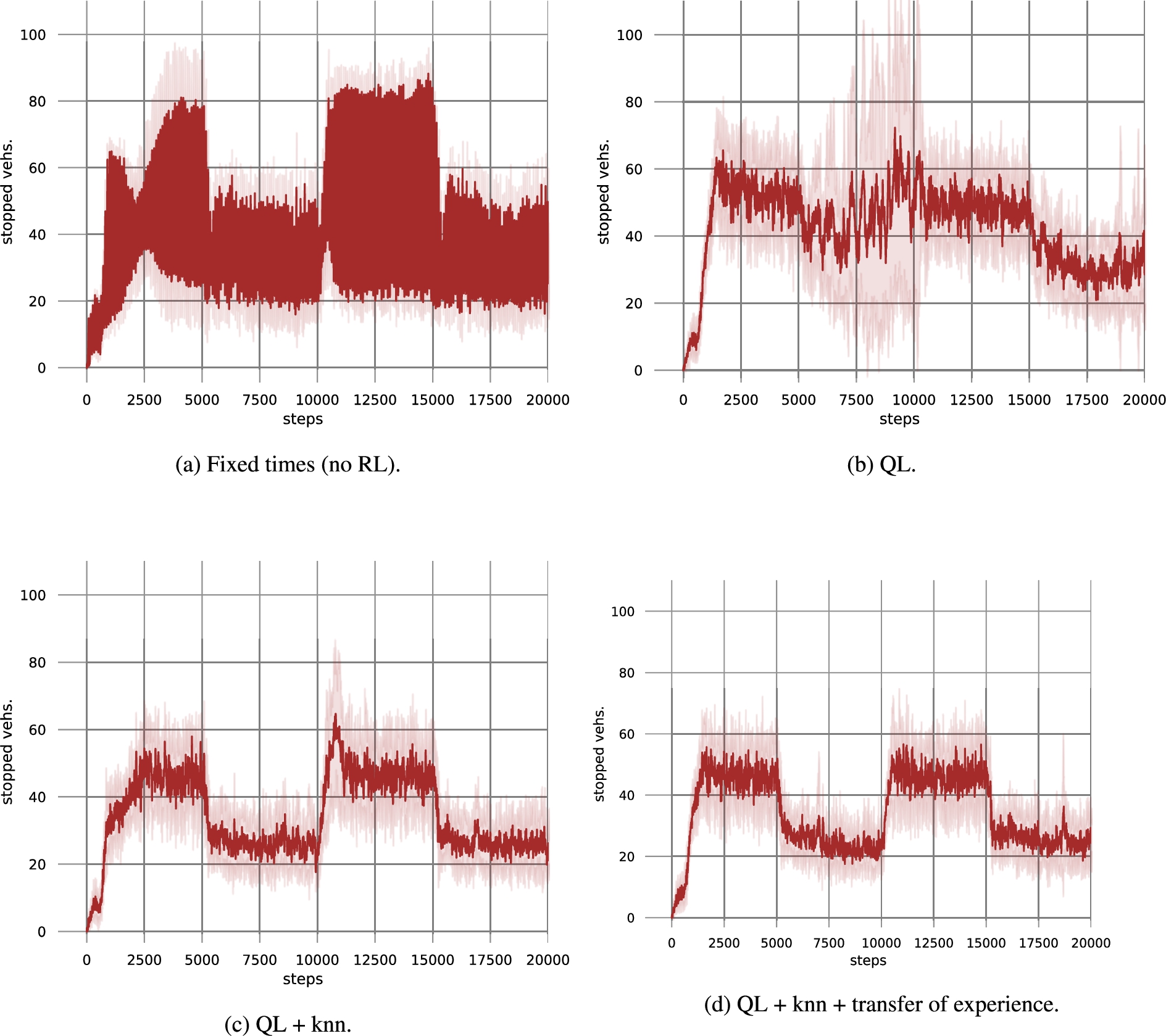
Comparison of the number of stopped vehicles in the network.

We compare our method to two baselines: fixed times and when only tabular Q-learning is used. For the former, we use a cycle of 90 seconds, splitting green time equally, so that each phase receives green for 42 seconds, and there is a 3 second red and yellow signal after each phase change. These values were computed by SUMO. For Q-learning, the values of α, γ, ε and the decay on ε mentioned in the previous section were used. In all cases, we have run 10 repetitions in order to show the deviations from the mean value.

We measure the number of stopped vehicles along time. For the two baseline situations, plots are depicted in Fig. 2a and Fig. 2b. For the sake of clarity, we show each situation in one plot, so that deviations are easily spotted.

One can observe that using fixed times (Fig. 2a) yields lots of oscillations, not only when contexts are changed, but virtually at all times. This is due to the fact that the rules to deal with the traffic volume are fixed, but the traffic volume itself changes.

The use of Q-learning without k-NN and/or communication among the agents does not produce such oscillations (see Fig. 2b) but: (i) it results in higher number of stopped vehicles, (ii) it does not adapt well and fast after there is a change from context 1 to context 2, and (iii) it produces the highest deviations (see shadow in lighter color).

Figure 2c shows the result when k-NN is used in conjunction with Q-learning. It is possible to notice that there is a reduction in the number of stopped vehicles – especially when there is a change to context 2 (at time step 5,000), which shows that the use of k-NN is able to adapt fast to such change. Notice also the reduction in the deviations (shadow) as compared to Fig. 2b.

Finally, Fig. 2d covers the result when agents communicate in order to transfer experiences when necessary. This is the case when they find themselves in states for which they do not have k good (meaning below the distance threshold) estimates to compute the Q-value. This is especially the case in the beginning of each never experienced context (i.e., at the initial time steps, as well as around step 5,000 when there is a change in context).

By comparing Fig. 2d to Fig. 2c, we do not see an improvement of performance: up to step 5,000, values are actually not much different. The fact that agents are still exploring with very high probabilities (as ε starts at 1.0) means that agents have values that are not necessarily good estimates for a Q-value, thus the transfer of such experiences do not improve the performance. However, once the environment goes back to context 1 (around 10,000), it is possible to see that transferring experiences pays off, even if the improvement is not big.

Overall, the number of stopped vehicles is lower when using transfer of experiences, in comparison to when k-NN is used without such transfer. And k-NN in conjunction with Q-learning does result in a better performance, when compared to when (tabular) Q-learning is used without k-NN. Moreover, all of them over-perform fixed times, as expected, given that this method does not adapt to changes in context.

7. Conclusion and future work

In this paper, we discuss how multiagent RL can be combined with k-nearest neighbors to estimate Q-values. This approach is particularly useful to deal with issues that arise when the state space is continuous and thus, a poor discretization may lead to poor performance. Further, we propose experience transfer among agents, in order to account for lack of good experiences. Besides proposing this approach, we illustrate its use with a scenario stemming from the area of traffic signal control, where we also deal with changes in context, i.e., in the traffic flow patterns.

Our results show that, compared to two baselines (one stemming from standard RL, i.e., a tabular method) the proposed approach performs better in terms of quality (less stopped vehicles), speed of convergence, and also presents less oscillations.

As discussed, transfering experiences led agents to improve their performance in a limited way, i.e., in given changes of context (but not in all). This may be due to the fact that agents have not yet found good estimates for some Q-values. Therefore, as a next step, we plan to extend the approach to incrementally cluster the agents’ experiences in order to have more abstract representation of the Q-values. This in turn can be helpful when sharing knowledge among the agents, since they may be able to do this at a higher abstraction level. Regarding the experiments, we intend to use scenarios in which agents are heterogeneous (e.g., they have a different set of actions that arise due to different set of phases).

Footnotes

Acknowledgements

We are thankful to the anonymous reviewers. This work is partially supported by FAPESP and MCTI/CGI (grants number 2020/05165-1) and by CAPES (Coordenação de Aperfeiçoamento de Pessoal de Nível Superior – Brazil, Finance Code 001). Vicente N. de Almeida was partially supported by a FAPERGS grant. Ana Bazzan is partially supported by CNPq under grant number 304932/2021-3, and by the German Federal Ministry of Education and Research (BMBF), Käte Hamburger Kolleg Cultures des Forschens/ Cultures of Research.

References

Abdoos and

A.L.C.

Bazzan, Hierarchical traffic signal optimization using reinforcement learning and traffic prediction with long-short term memory, Expert Systems with Applications (2021), 114580. doi:10.1016/j.eswa.2021.114580.

Abdoos,

Mozayani and

A.L.C.

Bazzan, Hierarchical control of traffic signals using Q-learning with tile coding, Appl. Intell.40(2) (2014), 201–213. doi:10.1007/s10489-013-0455-3.

L.N.

Alegre, SUMO-RL, GitHub, 2019.

L.N.

Alegre,

A.L.C.

Bazzan and

B.C.

da Silva, Quantifying the impact of non-stationarity in reinforcement learning-based traffic signal control, PeerJ Computer Science7 (2021), e575. doi:10.7717/peerj-cs.575.

L.N.

Alegre,

Ziemke and

A.L.C.

Bazzan, Using reinforcement learning to control traffic signals in a real-world scenario: An approach based on linear function approximation, IEEE Transactions on Intelligent Transportation Systems (2021). doi:10.1109/TITS.2021.3091014.

Aslani,

M.S.

Mesgari and

Wiering, Adaptive traffic signal control with actor-critic methods in a real-world traffic network with different traffic disruption events, Transportation Research Part C: Emerging Technologies85 (2017), 732–752. doi:10.1016/j.trc.2017.09.020.

Baird, Residual algorithms: Reinforcement learning with function approximation, in: Proceedings of the Twelfth International Conference on Machine Learning, Morgan Kaufmann, 1995, pp. 30–37.

P.G.

Balaji,

German and

Srinivasan, Urban traffic signal control using reinforcement learning agents, IET Intelligent Transportation Systems4(3) (2010), 177–188. doi:10.1049/iet-its.2009.0096.

A.L.C.

Bazzan, Opportunities for multiagent systems and multiagent reinforcement learning in traffic control, Autonomous Agents and Multiagent Systems18(3) (2009), 342–375. doi:10.1007/s10458-008-9062-9.

10.

Castagna and

Dusparic, Expert-free online transfer learning in multi-agent reinforcement learning, 2023, arXiv preprint arXiv:2303.01170.

11.

V.N.

de Almeida,

A.L.C.

Bazzan and

Abdoos, Multiagent reinforcement learning for traffic signal control: A k-nearest neighbors based approach, in: Twelfth International Workshop on Agents in Traffic and Transportation,

A.L.C.

Bazzan,

Dusparic,

Lujak and

Vizzari, eds, CEUR Workshop Proceedings, Vol. 3173, CEUR-WS.org, 2022, pp. 32–46, http://ceur-ws.org/Vol-3173/3.pdf .

12.

El-Tantawy,

Abdulhai and

Abdelgawad, Multiagent reinforcement learning for integrated network of adaptive traffic signal controllers (MARLIN-ATSC): Methodology and large-scale application on downtown Toronto, Intelligent Transportation Systems, IEEE Transactions on14(3) (2013), 1140–1150. doi:10.1109/TITS.2013.2255286.

13.

Han,

Jin,

Yang,

Cao and

Zhang, Research on robot motion control based on local weighted kNN-TD reinforcement learning, in: Proceedings of the 10th World Congress on Intelligent Control and Automation, 2012, pp. 3648–3651. doi:10.1109/WCICA.2012.6359080.

14.

Lin,

Shen,

Zhou,

Liu,

Zhang,

Xiao and

Cheng, KNN-Q learning algorithm of bitrate adaptation for video streaming over HTTP, in: 2020 Information Communication Technologies Conference (ICTC), 2020, pp. 302–306. doi:10.1109/ICTC49638.2020.9123312.

15.

P.A.

Lopez,

Behrisch,

Bieker-Walz,

Erdmann,

Y.-P.

Flötteröd,

Hilbrich,

Lücken,

Rummel,

Wagner and

Wießner, Microscopic traffic simulation using SUMO, in: The 21st IEEE International Conference on Intelligent Transportation Systems, 2018.

16.

Mannion,

Duggan and

Howley, An experimental review of reinforcement learning algorithms for adaptive traffic signal control, in: Autonomic Road Transport Support Systems,

Leo McCluskey,

Kotsialos,

P.J.

Müller,

Klügl,

Rana and

Schumann, eds, Springer International Publishing, Cham, 2016, pp. 47–66. doi:10.1007/978-3-319-25808-9_4.

17.

J.A.

Martín H. and

de Lope, A k-NN based perception scheme for reinforcement learning, in: Computer Aided Systems Theory – EUROCAST 2007,

R.M.

Díaz,

Pichler and

A.Q.

Arencibia, eds, Lecture Notes in Computer Science, Vol. 4739, Springer, Berlin, Heidelberg, 2007, pp. 138–145. doi:10.1007/978-3-540-75867-9_18.

18.

J.A.

Martín H.,

de Lope and

Maravall, The kNN-TD reinforcement learning algorithm, in: Methods and Models in Artificial and Natural Computation. A Homage to Professor Mira’s Scientific Legacy,

Mira,

J.M.

Ferrández,

J.R.

Álvarez,

de la Paz and

F.J.

Toledo, eds, Springer, Berlin, Heidelberg, 2009, pp. 305–314. ISBN 978-3-642-02264-7. doi:10.1007/978-3-642-02264-7_32.

19.

Noaeen,

Naik,

Goodman,

Crebo,

Abrar,

Far,

Z.S.H.

Abad and

A.L.C.

Bazzan, Reinforcement learning in urban network traffic signal control: A systematic literature review, 2021, engrxiv.org/ewxrj. doi:10.31224/osf.io/ewxrj.

20.

Odom,

Kumaraswamy,

Kersting and

Natarajan, Learning through advice-seeking via transfer, in: Inductive Logic Programming: 26th International Conference, ILP 2016, London, UK, September 4–6, 2016, Revised Selected Papers 26, Springer, 2016, pp. 40–51. doi:10.1007/978-3-319-63342-8_4.

21.

Papageorgiou,

Diakaki,

Dinopoulou,

Kotsialos and

Wang, Review of road traffic control strategies, Proceedings of the IEEE91(12) (2003), 2043–2067.

22.

R.P.

Roess,

E.S.

Prassas and

W.R.

McShane, Traffic Engineering, 3rd edn, Prentice Hall, 2004, p. 816.

23.

F.L.D.

Silva, Integrating agent advice and previous task solutions in multiagent reinforcement learning, in: Proceedings of the 18th International Conference on Autonomous Agents and MultiAgent Systems, 2019, pp. 2447–2448.

24.

F.L.D.

Silva and

A.H.R.

Costa, A survey on transfer learning for multiagent reinforcement learning systems, Journal of Artificial Intelligence Research64 (2019), 645–703. doi:10.1613/jair.1.11396.

25.

F.L.D.

Silva,

M.E.

Taylor and

A.H.R.

Costa, Autonomously reusing knowledge in multiagent reinforcement learning, in: Proceedings of the Twenty-Seventh International Joint Conference on Artificial Intelligence (IJCAI-18), IJCAI, 2018, pp. 5487–5493.

26.

R.S.

Sutton and

A.G.

Barto, Reinforcement Learning: An Introduction, 2nd edn, The MIT Press, 2018.

27.

M.E.

Taylor and

Stone, Transfer learning for reinforcement learning domains: A survey, Journal of Machine Learning Research10(56) (2009), 1633–1685.

28.

Torrey,

Shavlik,

Walker and

Maclin, Advice-based transfer in reinforcement learning, University of Wisconsin machine learning group working paper 06, 2, 2006.

29.

Van Der Pol, Deep reinforcement learning for coordination in traffic light control, PhD thesis, University of Amsterdam, 2016.

30.

Watkins, Learning from delayed rewards, PhD thesis, University of Cambridge, 1989.

31.

Wei,

Zheng,

Gayah and

Li, Recent advances in reinforcement learning for traffic signal control: A survey of models and evaluation, SIGKDD Explor. Newsl.22(2) (2021), 12–18. doi:10.1145/3447556.3447565.

32.

Wei,

Zheng,

V.V.

Gayah and

Li, A survey on traffic signal control methods, 2020, preprint arXiv:1904.08117.

33.

Wei,

Zheng,

Yao and

Li, IntelliLight: A reinforcement learning approach for intelligent traffic light control, in: Proceedings of the 24th ACM SIGKDD International Conference on Knowledge Discovery and Data Mining, KDD ’18, Association for Computing Machinery, New York, NY, USA, 2018, pp. 2496–2505. ISBN 9781450355520. doi:10.1145/3219819.3220096.

34.

K.-L.A.

Yau,

Qadir,

H.L.

Khoo,

M.H.

Ling and

Komisarczuk, A survey on reinforcement learning models and algorithms for traffic signal control, ACM Comput. Surv.50(3) (2017). doi:10.1145/3068287.

35.

Ye,

Zhu,

Cheng,

Zhou and

S.Y.

Philip, Differential advising in multiagent reinforcement learning, IEEE Transactions on Cybernetics52(6) (2020), 5508–5521. doi:10.1109/TCYB.2020.3034424.

Transferring experiences in k-nearest neighbors based multiagent reinforcement learning: an application to traffic signal control

Abstract

Keywords

1. Introduction

2. Background on traffic assignment and reinforcement learning

2.1. Reinforcement learning

2.2. RL-based traffic signal control

3. Related work

4. Combining and transferring nearest neighbors’ knowledge with Q-learning: General framework

4.1. Temporal difference learning based on k-nearest neighbors

4.1.1. Estimating Q-values

4.1.2. Action selection and updating Q-values

4.2. Communicating agents transferring experiences

4.3. Pseudo-code

5.1. Scenario

5.2.1. State space

5.2.2. Action space

5.2.3. Reward function

5.3. Changing the demand along the simulation horizon

2 Route route 4 involves a loop by design, in order to create more traffic at intersections C2 and D2.

6.1. Setting the values of the learning parameters

6.2. Results and discussion

Footnotes

Acknowledgements

References

²
Route ${route}_{4}$ involves a loop by design, in order to create more traffic at intersections C2 and D2.