Feature matching for 3D AR: Review from handcrafted methods to deep learning

Abstract

3D augmented reality (AR) has a photometric aspect of 3D rendering and a geometric aspect of camera tracking. In this paper, we will discuss the second aspect, which involves feature matching for stable 3D object insertion. We present the different types of image matching approaches, starting from handcrafted feature algorithms and machine learning methods, to recent deep learning approaches using various types of CNN architectures, and more modern end-to-end models. A comparison of these methods is performed according to criteria of real time and accuracy, to allow the choice of the most relevant methods for a 3D AR system.

Keywords

Feature detection feature descriptor image matching handcrafted and learned features 3D rendering augmented reality

1. Introduction

Image matching consists in accurately locating similar regions of images acquired from different viewpoints. An example of matching is shown in Fig. 1.

The applications of matching are numerous: the creation of a 3D map of a scene from a set of images acquired from different viewpoints by Structure From Motion (SfM) methods [50] or from a video by SLAM methods [42], geo-localization on a map by comparing an image to the images of a prerecorded 3D map, the creation of panoramas by merging multiple images into a single image [7], object detection [61], or autonomous drone controls [55].

The application that interests us in our work is the 3D augmented reality (AR) [22, 21], which consists in inserting 3D synthetic images in videos of real scenes.

The 3D augmented reality has a photometric aspect of 3D rendering and a geometric aspect of camera tracking.

1.1 3D rendering

3D rendering is used to illuminate the 3D objects, in such a way that it is inserted in a coherent way with the real scene. In [23], we presented the different traditional 3D rendering techniques of rasterization and ray tracing, and deep learning methods of Generative Adversarial Networks GAN, Variational Autoencoders VAE and the recent discipline of neural rendering, which combine the physical aspect of rendering and deep learning. A comparison was made according to different criteria of photo-realism, controllability, computational and working time, accessibility, quality of details and applications.

Figure 1.

Image matching example.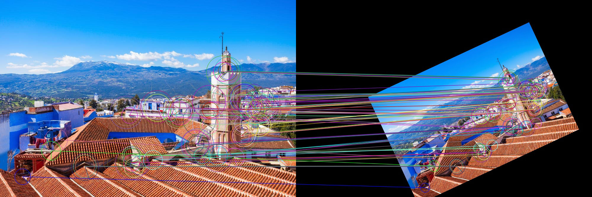

1.2 Feature tracking

The geometrical aspect of augmented reality is the goal of this article. The purpose of this step is to track the camera movement in order to be able to insert the 3D objects in a coherent way with the geometry of the scene. This is achieved by matching the features of the successive images of the video. Features (or keypoints) are locally unique regions in the image, such as corners or blobs.

The traditional feature matching pipeline consists of three main steps: detection, description and matching of image features.

Before presenting in detail image matching based on handcrafted, machine learning and deep learning methods, we will start by discovering the different types of approaches and their evolution.

Traditional methods, despite the advent of deep learning, are still used because of their performance. In [40], a sliding window is used to calculate the intensity variation of a block in several directions. In the Harris algorithm [27], the problem is reformulated to take into account all directions. The detection can be improved by sub-pixel accuracy algorithms. Multi-scale detection is proposed in [33]. Affine transformation invariant detectors are proposed in [36] and [35]. SIFT [34] allows detection and description of features, it is the most popular algorithm. The SURF algorithm [4] allows to accelerate SIFT by approximations with filters. ASIFT is a variant of SIFT [41] allowing to make the descriptor invariant by affine transformation. There are several fast detectors and descriptors such as FAST [47], BRIEF [9], ORB [48] and BRISK [32], their disadvantage is that they are less accurate.

The use of machine learning for the detection, description, and matching of features started a little before the “big bang” of deep learning. In [30], PCA is used to reduce the dimensionality of the SIFT descriptor. The drawback of PCA is that we do not have information about the labels of the classes. To solve this problem, it is possible to reduce the dimensionality of the descriptor with a linear discriminant analysis (LDA) as in [8]. In [52], the reduction of dimensionality is reformulated into convex optimization for better performance.

The method proposed in [28] is one of the first to use convolutional neural networks (CNN) for descriptor learning and feature matching. The goal is to train a Siamese network to identify similar patches of features. The dataset used is obtained by geometric and photometric image deformations. The success of deep learning for image matching is due to several factors: the possibility of using pre-trained CNNs on large datasets such as ImageNet [13], the CNNs are able to learn different image textures in each layer and the descriptors of the features can be obtained by removing the last layers (Fully Connected, etc.). In [18] it was shown that a CNN can achieve better matching results than SIFT. In [69] deeper architectures are used to improve performance. However, it was shown in [3] that performance can be improved with a shallow CNN (TFeat) by using triplets of training samples: reference patch, a positive (similar) patch, and negative (different) patch. A simple 6-layer CNN (L2-Net) was also used in [56] but with complex objective functions (loss function). The HardNet model proposed in [39], shows that with a simple objective function, but a more advanced training triplet selection strategy, it outperforms L2-Net. The SOSNet model [57] improves the performance by optimizing the intra- and inter-class distances. The most recent methods propose new architectures and strategies for matching [16, 5], homography estimation [31, 70], dense estimation [60, 59], or new models based on transformers [54, 29].

In other “modern” approaches, rather than using the classical pipeline (detection, description, matching) they use “end-to-end” training, unifying several parts of the pipeline in a differentiable way. In [66], a LIFT model is trained to perform both detection, orientation estimation, and description of features. The LF-Net model [44] uses the same principle with a different architecture. There are more and more models using this type of approach: Superpoint [14], IMIPs [12], DELF [43], D2-Net [15], UR2KiD [65] or SuperGlue [49]. In [67] a model is used to improve the matching by detecting outliers and which, combined with LIFT, shows performance that far exceeds the popular RANSAC method [19]. These modern approaches perform very well for complex images (large geometric variations and illumination) but the classical training pipeline based methods perform better in other simpler cases.

In this article we will present these different kind of approaches and a comparison according to different criteria of real time, accuracy, accessibility and applications, to allow the choice of the most relevant methods for a 3D augmented reality system.

In Section 1, we will present the traditional methods. Then, in Section 2, we will discover the methods based on machine and deep learning. Finally, in Section 3, we present the results of the comparison.

2. Handcrafted methods

2.1 Harris detector

In [40], a sliding window is used to compute the intensity variation of a block $W$ in several directions, looking for large variations, which correspond to corners. The mathematical formulation of the problem is as follows:

$\displaystyle E(u,v)=\sum_{x,y\in W}w(x,y)(I(x+u,y+v)-I(x,y))^{2}$ (1)

The function $E(u,v)$ measures the difference between the pixel intensities in a window $W$ and the intensities in $W$ shifted by a vector $(u,v)$ . The binary function $w(x,y)$ takes the value of $1$ inside the window and $0$ otherwise. The vector $(u,v)$ takes the values $[(1,1);(1,0);(0,1);(-1,1)]$ .

In the Harris algorithm [27], the problem is reformulated to take into account all directions. After a Taylor development of the Eq. (1) around $(u,v)=(0,0)$ and a matrix writing, we obtain:

$\displaystyle E(u,v)=\begin{bmatrix}u\\ v\end{bmatrix}^{T}\begin{bmatrix}\sum\limits_{x,y}w(x,y)\left(\frac{\partial I% (x,y)}{\partial x}\right)^{2}&\sum\limits_{x,y}w(x,y)\left(\frac{\partial I(x,% y)}{\partial x}\frac{\partial I(x,y)}{\partial y}\right)\\ \sum\limits_{x,y}w(x,y)\left(\frac{\partial I(x,y)}{\partial x}\frac{\partial I% (x,y)}{\partial y}\right)&\sum\limits_{x,y}w(x,y)\left(\frac{\partial I(x,y)}{% \partial y}\right)^{2}\end{bmatrix}\begin{bmatrix}u\\ v\end{bmatrix}$ (2)

The matrix in the right term, which we denote by $H$ , is called Harris matrix. The detection is realized by thresholding a quality function $C$ :

$\displaystyle C=\textit{det(H)}-\textit{k.Tr(H)}^{2}$ (3)

The parameter $k$ controls the sensitivity of the detector.

The drawback of the Harris detector is the fixed size of the window $W$ , which limits the detection to corners of the same size.

2.2 Multi-scale detection

The scale space theory is used in [33] to allow multiscale detection. The Harris matrix is reformulated by:

$\displaystyle H(x,y,\sigma_{D},\sigma_{I})=G(x,y,\sigma_{I})*\begin{bmatrix}% \left(\frac{\partial L(x,y,\sigma_{D})}{\partial x}\right)^{2}&\left(\frac{% \partial L(x,y,\sigma_{D})}{\partial x}\frac{\partial L(x,y,\sigma_{D})}{% \partial y}\right)\\ \left(\frac{\partial L(x,y,\sigma_{D})}{\partial x}\frac{\partial L(x,y,\sigma% _{D})}{\partial y}\right)&\left(\frac{\partial L(x,y,\sigma_{D})}{\partial y}% \right)^{2}\end{bmatrix}$ (4)

with $L$ the scale space set obtained by convolution of the image by multiple Gaussian $G(x,y,\sigma_{D})$ :

$\displaystyle L(x,y,\sigma_{D})=G(x,y,\sigma_{D})*I(x,y)$ (5)

and

$\displaystyle\frac{\partial L(x,y,\sigma_{D})}{\partial x}=\frac{\partial G(x,% y,\sigma_{D})}{\partial x}*I(x,y)$ (6)

The function $G(x,y,\sigma_{I})$ replaces the binary function $w$ to give more weight to the center pixels:

$\displaystyle w(x,y)=G(x-x_{0},y-y_{0},\sigma_{I})=\frac{1}{2\pi\sigma_{I}^{2}% }\exp\left(-\frac{1}{2\sigma_{I}^{2}}\left((x-x_{0})^{2}+(y-y_{0})^{2}\right)\right)$ (7)

with:

$\displaystyle\sigma_{I}=a.\sigma_{D}∼{},∼{}\textit{where}\hskip 14.226378pta% \in[1;2]$ (8)

The scale values used are:

$\displaystyle\{\sigma_{0},\sigma_{0}.b,\sigma_{0}.b^{2},\ldots\}$ (9)

with $\sigma_{0}=1.5$ and $b\in[1.2;1.4]$ . To compare features detected at different scales $\sigma_{D}$ and $\sigma_{D}^{\prime}$ , the matrix $H$ must be normalized by multiplying it by the factor $(\frac{\sigma_{D}}{\sigma_{D}^{\prime}})^{2}$ .

The selection of the most representative scale of the feature is performed by detecting the local maxima on the scale dimension of the normalized Laplacian:

$\displaystyle NL(x,y,\sigma_{D})=\left|\sigma_{I}^{2}\left(\frac{\partial^{2}G% (x,y,\sigma_{D})}{\partial x^{2}}+\frac{\partial^{2}G(x,y,\sigma_{D})}{% \partial y^{2}}\right)*I(x,y)\right|$ (10)

For better detection of blobs (similar connected regions), the Harris matrix can be replaced by the Hessian matrix normalized with respect to scale:

$\displaystyle S(x,y,\sigma_{D})=\sigma_{D}^{2}\begin{bmatrix}\frac{\partial^{2% }L(x,y,\sigma_{D})}{\partial x^{2}}&\frac{\partial^{2}L(x,y,\sigma_{D})}{% \partial x\partial y}\\ \frac{\partial^{2}L(x,y,\sigma_{D})}{\partial x\partial y}&\frac{\partial^{2}L% (x,y,\sigma_{D})}{\partial y^{2}}\end{bmatrix}$ (11)

The trace of $S$ which corresponds to the Laplacian of Gaussian LoG, is used for the detection instead of the quality measure $C$ , and at the same time for the scale selection.

Another method consists in using the determinant of $S$ for the detection and the LoG for the scale selection. This allows a better compromise between blob detection and edge rejection.

2.3 Subpixel accuracy

It is possible to improve the detection of features with sub-pixel accuracy.

We start by detecting the connected components in the measurement quality map $C$ , where several points may correspond to the same corner. We look for the point $q$ that minimizes:

$\displaystyle\epsilon_{i}=\nabla I_{p_{i}}\bullet(q-p_{i})$ (12)

Indeed, if $q$ is in the corner and $p_{i}$ in the neighborhood of $q$ , we have two cases:

•

if $p_{i}$ is in a line: the gradient $\nabla I_{p_{i}}$ is perpendicular to $q-p_{i}$ , then $\epsilon_{i}=0$ .

•

if $p_{i}$ is in a uniform region: the gradient $\nabla I_{p_{i}}=0$ , and therefore $\epsilon_{i}=0$ .

In practice $\epsilon_{i}$ will never be zero because of the noise, so we proceed by minimization. We thus seek in the neighborhood $V_{q}$ of $q$ to minimize the function $E$ obtained after developing the Eq. (12):

$\displaystyle E=\sum_{i\in V_{q}}(\nabla I_{p_{i}}.\nabla I_{p_{i}}^{T}).q-% \sum_{i\in V_{q}}(\nabla I_{p_{i}}.\nabla I_{p_{i}}^{T}).p_{i}$ (13)

We note:

$\displaystyle G=\sum_{i\in V_{q}}(\nabla I_{p_{i}}.\nabla I_{p_{i}}^{T})$ (14) $\displaystyle b=\sum_{i\in V_{q}}(\nabla I_{p_{i}}.\nabla I_{p_{i}}^{T}).p_{i}$ (15)

If $E=0$ , we obtain:

$\displaystyle q=G^{-1}.b$ (16)

The algorithm is as follows:

We start by initializing $q$ with the center of the connected region.

We compute in the neighborhood of $q$ the values of $G$ and $b$ .

We compute the new $q=G^{-1}.b$ (or we minimize $E$ by least squares).

We calculate the error $q-q_{previous}$ . If the error is less than a threshold, we stop the calculation, otherwise we start again at step 2.

2.4 MSER

MSER (Maximally Stable Extremal Region or MSER) [35] is a covariant blob detector by affine transformation. The principle is to vary a threshold $i$ and to find the $\Omega$ regions such that:

$\displaystyle\forall p\in\Omega,\forall q\in V_{\Omega},\ I(p)<I(q)\ \textit{% or}\ I(p)>I(q),$ (17)

with $V_{\Omega}$ the neighborhood of $\Omega$ . In other words, the pixels connected inside the detected regions are all brighter or darker than the pixels of the external contours. As the threshold $i$ increases, the size of the regions increases. The detection of the features is performed by selecting the stable regions for matching, which correspond to the regions obtained with the threshold $i$ that minimizes the measurement:

$\displaystyle q(i)=\frac{\textit{Card}(\Omega_{i+1}-\Omega_{i-1})}{\textit{% Card}(\Omega_{i})}$ (18)

with $\textit{Card}(\Omega_{i})$ is the area of the region $\Omega_{i}$ and $\Omega_{i}\subset\Omega_{i+1}$ .

The ellipse surrounding the detected region is used as the feature patch. Stable regions have the property of remaining connected after affine transformation and are therefore reliable for matching.

2.5 FAST

The FAST algorithm [47] allows fast detection of the corners, thanks to a thresholding on a circle of $16$ pixels.

We consider a region to be a Feature if at least $12$ pixels of the circle satisfy the condition:

$\displaystyle I_{x}>I_{p}+t,$ (19)

or:

$\displaystyle I_{x}<I_{p}-t,$ (20)

with $I_{x}$ the intensity of a pixel of the circle, $I_{p}$ the intensity of the central pixel and $t$ a threshold. A preselection of features is performed on pixels $1$ , $5$ , $9$ and $13$ of the circle. It is necessary that at least $3$ among these pixels verify the previous condition. If this is the case, we apply the test on the $16$ pixels. The algorithm for removing non-local maxima can be applied by considering the following measure:

$\displaystyle V=\sum_{i=1}^{16}|I_{p}-I_{x}|$ (21)

If two features have close positions, we eliminate the one with the lowest value of $V$ . Note that it is possible to train a machine learning algorithm with FAST. For this, a decision tree is built by applying FAST on a set of training images, in order to generate the decision tree that we then use to detect features on new images. The drawback of FAST is that it is very sensitive to noise.

2.6 SIFT

2.6.1 Feature detection and scale selection

The detection in SIFT [34] is performed by the LoG operator (seen previously), which is approximated by difference of Gaussian (DoG) by introducing the notion of octave. DoG with different $\sigma$ of the scale space $(\sigma,k.\sigma,k^{2}.\sigma,k^{3}.\sigma,,k^{4}.\sigma)$ are applied to detect corners and blobs of different sizes (low $\sigma$ for small corners and high $\sigma$ for large corners). The octaves allow to go to the next scale without modifying the parameters $(\sigma,k.\sigma,k^{2}.\sigma,k^{3}.\sigma,,k^{4}.\sigma)$ , but by reducing the resolution of the image, which allows to accelerate the calculations. The $\sigma$ scale which forms a local extremum with the previous and following scales, as well as spatially (neighboring pixels) corresponds to a potential feature.

2.6.2 Feature localization

The problem with the result of the previous step is the lack of accuracy in locating the features. Indeed, because of the use of a discrete space of scales $(\sigma,k.\sigma,k^{2}.\sigma,k^{3}.\sigma,,k^{4}.\sigma)$ , the position of the extrema is not very exact. The true extrema are localized by a Taylor expansion. Then, a threshold is applied to the DoG matrices to eliminate the weak contrasts. Another problem of the DoG operator is that it detects many edges. However, for the edges, the eigenvalues of the Hessian matrix verify $\lambda_{1}\gg\lambda_{2}$ . So we compute the ratio $\frac{\lambda_{1}}{\lambda_{2}}$ . If the ratio is higher than a threshold $r$ , then it is a edge. We can also use the Hessian matrix with the condition:

$\displaystyle\frac{\textit{Tr(H)}}{\textit{Det(H)}}<\frac{(r+1)^{2}}{r}$ (22)

Note that SIFT is a good blob detector, while Harris is a good corner detector.

2.6.3 Feature orientation and descriptor

Once we have obtained the position and scale of the feature, we compute a descriptor $D e s c$ . Let $f$ and $f^{\prime}$ be two features in two different images such that $f^{\prime}=T(f)$ , with $T$ a geometric and photometric transformation (change of viewpoint, scale, rotation or luminance variation). A good descriptor $D$ must verify $Desc(f)=Desc(f^{\prime})$ .

We start by choosing the relevant pixels that will contribute to the calculation of the descriptor. We consider a support region, larger than the scale around the detected feature. Then, in order to be able to compare the descriptors of two features with different orientations, we detect in each support region the orientation of the dominant gradient, and we change the orientation so that the dominant gradient is horizontal. To detect the orientation of the dominant gradient, we first compute the magnitude $M$ and the orientation $\theta$ of the gradient for each pixel in the support region $D$ :

$\displaystyle M(x,y)=\sqrt{(D(x+1,y)-D(x-1,y))^{2}+(D(x,y+1)-D(x,y-1))^{2}}$ (23) $\displaystyle\theta=\arctan\left(\frac{D(x,y+1)-D(x,y-1)}{D(x+1,y)-D(x-1,y)}\right)$ (24)

A region $16\times 16$ is considered around the feature. This region is divided in sub-regions $4\times 4$ . For each sub-region we create the orientation histogram on $8$ bins. Each pixel is incremented by the magnitude $M$ weighted by a Gaussian $M(x,y).G(x,y,\sigma)$ to give more weight to the center pixels. With $\sigma$ equal to $1.5$ times the scale of the Feature. We thus obtain a vector descriptor of $128$ values ( $8\times 16$ ).

Note that there are other methods, using similar principles to SIFT for the calculation of the descriptor, but with different patch shapes: GLOH [37], CHOG [10] and DAISY [58].

2.7 ASIFT

ASIFT [41] is a SIFT variant allowing to make the descriptor invariant by affine transformation. The principle is to apply for each feature patch different affine transformations, and during the matching, we compare it to all the patchs in the other image. The disadvantage is that the calculation is very expensive. Note that there are also affine variants of the multi-scale Harris detectors, but the ASIFT detector gives better results.

2.8 SURF

The SURF algorithm [4] accelerates SIFT by approximating the LoG operator with filters. First, the second derivatives of a Gaussian $\frac{\partial^{2}g(\sigma)}{\partial x^{2}}$ , $\frac{\partial^{2}g(\sigma)}{\partial y^{2}}$ and $\frac{\partial^{2}g(\sigma)}{\partial x\partial y}$ are approximated by simple filters. Then we just have to replace the Hessian matrix $S$ of the Eq. (11) by its approximation. The Hessian matrix becomes:

$\displaystyle S_{\textit{approx}}(x,y,\sigma_{D})=\sigma_{D}^{2}\begin{bmatrix% }D_{xx}&D_{xy}\\ D_{xy}&D_{yy}\end{bmatrix}$ (25)

with:

$\displaystyle D_{xx}=\frac{\partial^{2}G(x,y,\sigma_{D})}{\partial x}*I(x,y),$ (26)

such that $\frac{\partial^{2}G(x,y,\sigma_{D})}{\partial x}$ is approximated by a filter. The detection of features and scale is performed as before by the determinant of $S$ .

Note that the summed area table algorithm is used for the fast computation of sums in the filtering operation.

The octave scale space theory is used, except that instead of decreasing the image size, the filter size is increased. The lowest level corresponds to a filter of size $9\times 9$ which is equivalent to a Gaussian with a $\sigma=1.2$ .

In [4], the formula of the determinant of the hessian, used for scale detection is approximated by:

$\displaystyle\textit{det}(S_{\textit{approx}})=D_{xx}D_{yy}-0,9D_{xy}$ (27)

The orientation of the features is detected with Haar wavelets by calculating the sum of the horizontal and vertical wavelet responses, over a $6.\sigma$ neighborhood around the feature, with a step size of $\frac{\pi}{3}$ . The orientation corresponds to the largest sum. The integral sum is used again to speed up the computation.

For the descriptor, we consider a neighborhood of size $20\sigma$ around the feature and we divide it in $16$ regions ( $4\times 4$ ). Haar wavelets are applied on each region in order to compute a vector of size $4$ : $[\sum I_{i},\sum|I_{i}|,\sum I_{j},\sum|I_{j}|]$ . We finally obtain a vector of size $64$ for the $16$ regions which corresponds to our SURF descriptor.

Note that there is an extended SURF version with $128$ dimensions such that the sums are computed for $dx>0$ and $dx<0$ separately and similarly for $d y$ .

Note finally that the sign of the Laplacian allows to distinguish between black blobs on white background and the opposite. This is useful for matching only blobs of the same type.

2.9 BRIEF

The disadvantage of the SIFT and SURF descriptors is that they are stored with $32$ bit float values. So for each $128$ Feature, we need $512$ bytes.

There are solutions consisting in applying a PCA (Principal Component Analysis) or LDA (Linear Discriminant Analysis) in order to reduce the dimensionality of the vector, or to apply a LSH (Locality sensitive hashing) algorithm to convert the vector into binary. However, we still have to calculate the descriptor in float first.

The principle of the BRIEF descriptor [9] consists in selecting $n$ pairs of points $(p,q)$ in a patch of the image (smoothed). The selection is performed according to uniform Gaussian distributions. If $I_{p}>I_{q}$ , then the descriptor element takes the value of $1$ , otherwise it takes the value of $0$ . We apply this to all $n$ pairs to obtain a descriptor of dimension $n$ . The matching can be done in the case of binary descriptors using the Hamming distance:

$\displaystyle\textit{dist}_{i,j}=\#\{i\neq j\}$ (28)

Note that unlike SIFT and SURF, the BRIEF algorithm only allows the description of features. Detection can be done with another detector (Harris, SIFT, etc.), but the author recommends the CenSurE algorithm [1].

2.10 ORB

The ORB algorithm [48] is a combination of the FAST detector and the BRIEF descriptor with some modifications to allow fast, multiscale, and rotation-invariant detection. First, the detection is performed with FAST. Then, the best $N$ points are selected using the Harris quality measure.

The detection is performed at several scales using a pyramid of images at different resolutions.

The orientation is computed as the direction between the center of the corner and the centroid of the patch computed from the first order moment:

$\displaystyle\textit{centroid}=\left(\frac{m_{10}}{m_{00}},\frac{m_{01}}{m_{00% }}\right),$ (29)

with:

$\displaystyle m_{pq}=\sum_{x,y}x^{p}y^{p}I(x,y)$ (30)

Thus, the orientation of the Feature is:

$\displaystyle\theta=\textit{atan2}(m_{01},m_{10})$ (31)

The BRIEF descriptor is modified to rBRIEF (rotation-aware BRIEF) to take into account the orientation of the Feature. The rotation matrix, corresponding to the angle $\theta$ , is applied to the patch before computing the BRIEF descriptor, in order to make it rotation invariant.

According to the author, the performances of ORB are quite close to SIFT, better than SURF and faster than both.

3. Machine and deep learning methods

3.1 PCA-SIFT

PCA-SIFT [30] is a variant of SIFT whose goal is to reduce the dimensionality of the descriptor by using a projection matrix estimated by training. This method has the advantage of being more accurate and faster than SIFT.

A pre-processing is first applied:

1)
SIFT detection of feature patches $41\times 41$ and reorientation with respect to the dominant gradient.
2)
Extraction of vertical ( $39\times 39$ ) and horizontal ( $39\times 39$ ) gradient maps.
3)
Vectorization and concatenation (( $2\times 39\times 39$ ) = $3042$ ).
4)
Unit normalization to reduce luminance variations.

Then, the principle is to use a training set of $N$ patches in order to create a data matrix $X$ (of size $N\times D$ ), composed of $N$ descriptors of dimension $D$ (here equal to $3042$ ). The goal is to reduce the descriptor dimension from $D$ to $K$ .

After normalization of $X$ (subtraction of the mean), we compute the covariance matrix $C$ of $X$ :

$\displaystyle C=X^{T}X$ (32)

We apply the singular value decomposition:

$\displaystyle C=U\Sigma V$ (33)

We use the first $K$ columns $U^{\prime}$ of $U$ (eigenvectors) to project a descriptor $x$ of a new feature (not in the training data) from space of dimension $D$ into a new space of dimension $K$ :

$\displaystyle x^{\prime}=U^{\prime T}x$ (34)

As shown in [30], compared to SIFT, PCA-SIFT improves the matching performance. The descriptor size is reduced from $3042$ to $20$ for maximum performance. When $K>40$ , the performances drop because useless information is considered.
3.2 Convex optimization

In [52], a method for learning descriptors by convex optimization is proposed. The algorithm is as follows.

The detected feature patch $x$ (by SIFT, Harris or other) is rectified with respect to the orientation of the dominant gradient and the affine deformation.

The orientation gradients of each pixel of the patch are computed as in SIFT on $p$ directions (bins) between $0$ and $2\pi$ . We thus obtain $p$ gradient images.

Each gradient image is convolved with a set of kernels, called “pooling regions”, having different support and positions. The pooling regions used are defined by:

$\displaystyle k(u,v;\rho,\alpha,\sigma)\sim\exp\left(-\frac{(u-\rho\cos(\alpha% ))^{2}+(v-\rho\sin(\alpha))^{2}}{2\sigma^{2}}\right),$ (35)

with $(u,v)$ the pixel coordinates and $(\rho,\alpha)$ the polar coordinates of the Gaussian of standard deviation $\sigma$ .

As a result of the convolutions, we obtain a descriptor $\Phi(x)$ of dimension $p . q$ , with $q$ the number of kernels.

Not all the pooling regions are used for training. A selection strategy is defined.

The descriptor is separated into several elements corresponding to each region:

$\displaystyle\phi_{i,j,c}(x)=\sqrt{w_{i}}.\Phi_{i,j,c}(x),$ (36)

with $i$ the circle (of pooling region) index, $j$ the kernel index, and $c$ the channel number. $w_{i}$ is a binary region selection mask: $w_{i}=1$ if the region is selected, otherwise $w_{i}=0$ .

The regions relevant for matching are selected by training. The training set is separated into two sets $P$ and $N$ , respectively, of positive patch pairs (similar) and negative patch pairs (different). We add a constraint that maximizes the distance between these two sets:

$\displaystyle d(\textbf{x},\textbf{y})+1<d(\textbf{u},\textbf{v}),\ \forall(% \textbf{x},\textbf{y})\in P\ \textit{and}\ \forall(\textbf{u},\textbf{v})\in N,$ (37)

with $d$ is the $L_{2}$ distance between the descriptors:

$\displaystyle d(x,y)=\sum_{i,j,c}(\sqrt{w_{i}}.\Phi_{i,j,c}(x)-\sqrt{w_{i}}.% \Phi_{i,j,c}(y))^{2}$ (38)

From these last two equations, we end up with a convex optimization problem that consists in finding relevant regions $w$ by minimizing by training the following objective function:

$\displaystyle\mathop{\text{missing}}{argmin}\limits_{w\geqslant 0}\sum_{(% \textbf{x},\textbf{y},\textbf{u},\textbf{v})}\mathcal{L}(w^{T}(\psi(\textbf{x}% ,\textbf{y})-\psi(\textbf{u},\textbf{v})))+\mu_{1}||w||_{1}$ (39)

such that:

$\displaystyle\psi(\textbf{x},\textbf{y})=\sum_{j,c}(\Phi_{i,j,c}(x)-\Phi_{i,j,% c}(y))^{2}$ (40)

and:

$\displaystyle\mathcal{L}(z)=\textit{max}(z+1,0)$ (41)

the regularization term $\mu_{1}||w||_{1}$ forces $w=0$ .

The optimization thus allows us to find the relevant regions $w$ for the matching.

Finally, we compute the descriptor:

$\displaystyle\tilde{\Phi}=\sqrt{w}\Phi$ (42)

The descriptor is also normalized to make it invariant to luminance changes, with respect to the mean and variance of the patch gradients or with the quantile of the gradient.

For dimensionality reduction, we look for a projection matrix $W$ which, in addition to reducing the dimension of the descriptor, allows to separate positive and negative pairs. This is equivalent to adding, in a similar way to what has been done before, the constraint:

$\displaystyle d_{W}(\textbf{x},\textbf{y})+1<d_{W}(\textbf{u},\textbf{v}),\ % \forall(\textbf{x},\textbf{y})\in P\ \textit{and}\ \forall(\textbf{u},\textbf{% v})\in N,$ (43)

with $d_{W}$ the distance between pairs after projection with $W$ :

$\displaystyle d_{W}(x,y)=||W.\phi(\textbf{x})-W.\phi(\textbf{y})||_{2}^{2}$ (44)

after development:

$\displaystyle d_{W}(x,y)=\theta(\textbf{x,y})^{T}.A.\theta(\textbf{x,y})$ (45)

with:

$\displaystyle\theta(\textbf{x,y})=\phi(\textbf{x})-\phi(\textbf{y})$ (46)

and

$\displaystyle A=W^{T}.W$ (47)

The problem is reformulated as before in convex optimization:

$\displaystyle\mathop{\text{missing}}{argmin}\limits_{A\geqslant 0}\sum_{(% \textbf{x},\textbf{y},\textbf{u},\textbf{v})}\mathcal{L}(\theta(\textbf{x,y})^% {T}.A.\theta(\textbf{x,y})-\theta(\textbf{u,v})^{T}.A.\theta(\textbf{u,v}))+% \mu_{\star}||A||_{\star}$ (48)

with $||A||_{\star}$ is the nuclear norm of $A$ , which corresponds to the sum of the singular values of $A$ . The regularization parameter $\mu_{\star}$ allows to set the dimension of the projection space which will corresponds to the rank of $A$ .

The optimization of the two objective functions Eqs (48) and (39) is performed by the RDA algorithm because of the size of the training samples and the use of sums. RDA is efficient for optimization problems of the form:

$\displaystyle\mathop{\text{missing}}{argmin}\limits_{w}\frac{1}{T}\sum_{t=1}^{% T}f(w,z_{t})+R(w)$ (49)

with $z_{t}$ is the $t$ -th sample and $R(w)$ the regularization term.

All the details of the updates of the parameters $w$ and $A$ of the Eqs (39) and (48) by RDA are available in [52].

3.3 CNN training based matching

In [28], two convolutional neural networks (CNN) architectures are proposed for descriptor training and for matching.

The dataset used is created by geometric transformations applied on a set of patches extracted by DoG (as in SIFT). The use of synthetic transformations has the advantage, compared to traditional methods, of controlling the amount of invariance of the transformations we want the model to learn.

In order to retain only reliable features for matching during training, a random homography is applied to each image. Given the known homography, we can deduce the position of each pixel in the second image. DoG detection is performed on the transformed image and a comparison is made with the position, scale and orientation of the features in the reference image. Position, scale and orientation tolerance thresholds are used. If the features are close, they are considered reliable for matching and are retained as training samples.

CNN architecture 1: The first description model receives at its input a patch $X$ of feature and, using a mapping function $G_{w}(X)$ , it returns at its output a descriptor of dimension $n$ which allows to do the matching. Indeed, this model must be trained on the patches of each image we want to match, by applying the geometrical transformations as previously.

This model can be seen as a classifier where each element at its output corresponds to a class (stable feature number).

The CNN is trained thus with all the patches of the stable features with the corresponding labels.

During the test phase, we provide the model with a patch of a new point of view image and it assigns it the closest class (matching).

CNN architecture 2: The second model uses a Siamese architecture consisting of two CNNs similar to the previous model, trained with the same parameters and each receiving a patch. The Euclidean distance $E_{w}$ between the two descriptors is computed. The objective function $\mathcal{L}$ of the Eq. (50) to be optimized during training, allows to compute the classification error of the pairs of patches as similar or different.

$\displaystyle\mathcal{L}=(1-Y)\frac{2}{Q}E_{w}^{2}+2YQ\exp\left(-\frac{2,77}{Q% }E_{w}\right),$ (50)

with $Y$ the label of the matching, such that $Y=1$ for different patches, otherwise $Y=0$ .

A similar architecture is used in [11] for person identification from face images.

The ground truth used for the evaluation uses the homographies of the dataset in [37]. The use of a model to do the training directly on the image to be processed allows to improve the performances, moreover we find a similarity with the ASIFT method. The disadvantage is that the number of features varies from one image to another, while the output size of the CNN is not directly adjustable. Architecture 2 has the advantage of offering a smaller descriptor size of 128. The disadvantage of both methods is the slow training and processing time.

3.4 CNN descriptors and evaluation metrics

In [18], a CNN is used for feature description based on the output of the hidden layers of a CNN trained for classification.

Two models are trained by supervised learning on the ImageNet dataset [13] and unsupervised learning (images without labels). The evaluation is performed on the dataset [38] and on a new dataset. The results show that the method outperforms SIFT and that unsupervised learning gives better results than supervised learning.

The supervised model uses a 5-layer CNN architecture, plus two fully connected layers (FC) and a softmax classification layer.

The unsupervised model is trained with $N=16000$ patches (randomly extracted) of dimension $64\times 64$ . $N$ is the number of classes. Each sample is augmented with 150 scale, color, contrast and rotation transformations. To avoid overfitting, a shallow model with 3 layers and a fully connected (FC) layer are used.

Note that both models have been trained for classification and the goal is to use the output of the hidden layers as a descriptor.

Feature detection is first performed by the MSER algorithm. Then, the descriptors are extracted from a hidden layer of the model. Finally, the matching is performed by comparing the Euclidean distances of the descriptors.

For evaluation, the matched patches are compared to the ground truth and are classified as true positive/negative (TP/TN) if they have an IOU (Intersection Over Union) of the MSER ellipses of at least $0.6$ , otherwise they are classified as false positive (FP):

$\displaystyle\textit{IOU}=\frac{\textit{Aire∼{}d'intersection}}{\textit{Aire∼{% }d'union}}$ (51)

Note that this metric is generally used for localization problems.

The IOU allows us to calculate the number of TP and FP according to the chosen threshold.

We can therefore deduce the precision and recall values from TP, FP and FN (false negative):

$\displaystyle\textit{Precision}=\frac{\textit{TP}}{\textit{TP}+\textit{FP}}$ (52) $\displaystyle\textit{Recall}=\frac{\textit{TP}}{\textit{TP}+\textit{FN}}$ (53)

Mean Average Precision metric:

The evaluation metric AP (Average Precision) is the area below the Precision-Recall curve. We then derive mAP (Mean Average Precision) by averaging the AP (over all classes and/or IOU thresholds).

These metrics are the most used for the evaluation of the matching methods.

Several hidden layers have been evaluated with this metric for the calculation of descriptors. The evaluation results show that in the case of unsupervised learning, the upper layers give better results. In the case of supervised learning, the results are similar whatever the layer used for the extraction of the descriptors, however, the size of the patches used has more influence on the results. The larger patch sizes are preferable in the case of CNNs.

CNNs give better matching results than SIFT but are slower.

3.5 CNN based matching by similarity function

In [69], a CNN is trained to learn a similarity function from patch pairs. A dataset is labeled in similar and different pairs. four architectures are proposed.

The first simple model uses a single CNN: the two patches are considered as a single two-channel image.

In the second Siamese model, two CNNs with the same weights are applied to the two patches (the two CNNs have shared branches). The two outputs are concatenated into a single vector of dimension $512$ , used as input of the FC layer. The output of the hidden layers corresponds to the descriptor and the last output to the similarity measure.

The third pseudo-Siamese model is similar to the previous one, with the difference that the two CNNs do not share the branches, which means that the weights of the 2 CNNs are different (implies more parameters).

The choice of the architecture depends on the speed of calculation and the accuracy.

For the matching, the FC layer can be replaced by a $L_{2}$ distance.

Other models can be combined with these architectures to create very deep and more powerful models [53]. The interest is to replace layers with large filter sizes, with several $3\times 3$ filters separated by ReLUs. This increases the non-linearity of the decision boundary.

The fourth model “Central-Surround” allows to perform a multi-scale matching. Two Siamese models are used. The “Surround” model receives the subsampled patches at a lower resolution (from $64\times 64$ to $32\times 32$ ) and thus allows a low resolution processing. The “Central” model receives the central part $32\times 32$ of the original patch and thus allows a higher resolution processing.

The Spatial Pyramid Pooling (SPP) method can be used to avoid resizing the patch. This consists in adding to the output of the CNNs a max-pooling layer of dimension proportional to the patch, which allows to keep all the information of the patch.

The training of the different models is performed by optimizing the following objective function:

$\displaystyle\textit{min}_{w}\frac{\lambda}{2}||w||_{2}+\sum_{i=1}^{N}\textit{% max}(0,1-y_{i}o_{i})$ (54)

with $w$ the model weights, $o_{i}$ the prediction of the $i$ -th sample and $y_{i}$ the labels ( $y_{i}=1$ for similar patches, otherwise $y_{i}=-1$ ), and $\lambda$ the regularization coefficient.

The evaluation results show better performance than convex optimization, SIFT and DAISY.

3.6 CNN matching by triplets of patches and hard negatives

In the TFeat model [3], patch triplet samples are used instead of patch pairs for CNN descriptor training.

In the precedent case of patch pairs, we use samples pairs $\{x_{1},x_{2}\}$ and the corresponding label $l=\{1,-1\}$ (similar or different). For a patch $x$ of dimension $m\times n$ , we look for a descriptor $f(x)$ , such that the distance $f(x_{1})-f(x_{2})$ is small if the two patches are similar and large otherwise. This is achieved by using an objective function “Contrastive Loss”:

$\displaystyle\mathcal{L}=\begin{cases}||f(x_{1})-f(x_{2})||_{2}∼{}∼{},\text{if% }∼{}∼{}l=1\\ \textit{max}(0,\mu-||f(x_{1})-f(x_{2})||_{2})∼{}∼{},\text{if}∼{}∼{}l=-1\end{% cases}\,.$ (55)

with $\mu$ the margin. $\mathcal{L}$ penalizes positive pairs that are separated by a large distance, as well as very close negative pairs (distance less than $\mu$ ).

The disadvantage of using pairs is that most negative pairs do not contribute to the gradient update during the optimization, since the distance is most often greater than $m u$ (because of random patches).

A solution [51] is to identify the “Hard Negative” pairs from their distances (close negative pairs) to use them mostly during the training. The disadvantage of this method is that it is time consuming.

In the case of triplets, we use sample sets $\{a,p,n\}$ with $a$ the reference patch (anchor), $p$ a patch similar to $a$ (positive) and $n$ a patch different from $a$ (negative). We note:

$\displaystyle\delta_{+}=||f(a)-f(p)||_{2}$ (56)

and

$\displaystyle\delta_{-}=||f(a)-f(n)||_{2}$ (57)

We use the objective function:

$\displaystyle\lambda(\delta_{+},\delta_{-})=\text{max}(0,\mu+\delta_{+}-\delta% _{-})$ (58)

This is equivalent to adjusting the weights of a CNN by optimizing the objective function to obtain:

$\displaystyle\delta_{-}>\delta_{+}+\mu$ (59)

This results in a distance $\delta_{-}$ between negative pairs that is larger, by a margin $\mu$ , than the distance $\delta_{+}$ between positive pairs.

A strategy to use the “Hard Negatives” is proposed to increase also the distance between $p$ and $n$ . For that we compute the distance:

$\displaystyle\delta^{\prime}_{-}=||f(p)-f(n)||_{2}$ (60)

We define the “Hard Negative” of triplets by:

$\displaystyle\delta_{*}=\text{min}(\delta_{-},\delta^{\prime}_{-})$ (61)

If $\delta_{*}=\delta^{\prime}_{-}$ , we swap $a$ and $p$ so that $p$ becomes the reference and $a$ the positive patch. This ensures that the “Hard Negative” of the triplets is used for the backpropagation of the gradient.

We thus obtain a new objective function:

$\displaystyle\lambda(\delta_{+},\delta^{\prime}_{*})=\text{max}(0,\mu+\delta_{% +}-\delta_{*})$ (62)

This method gives better results than those using patch pairs. The processing time on GPU is $10\mu s$ per patch.

3.7 L2-Net: Similarity, compactness and intermediate losses

The L2-Net model [56] uses an architecture with only convolutional layers followed by Batch Normalization layers and a LRN (Local Response Normalization) layer at the output.

For training, the datasets Brown [6] and HPatches [2] are used.

In practice, when we do the matching, we end up with many more different patches than similar patches. Because of the large number of negative patches it is impossible to use all of them for training. The previous methods use positive and negative classes with equal numbers of samples, while to be closer to reality we need more negative samples.

The strategy to select the relevant negative patches in larger quantities is the following:

1)
We consider a number $P$ of 3D points indexed $i$ of the scene and the corresponding $x^{j}_{i}$ patches in the images indexed $j$ .
2)
Iteratively, we sequentially select $p_{1}$ points from the set of $P$ points, and randomly select $p_{2}$ points from the remaining $P-p_{1}$ . The random selection increases the chances of the CNN learning new features and improving what it has already learned.
3)
For each point $i$ we randomly choose a pair $(x_{i}^{1},x_{i}^{2})$ from the set of $p=p_{1}+p_{2}$ selected points. We thus obtain a training batch of $p$ pairs of patches:

$\displaystyle X=\{x^{1}_{1},x^{2}_{1},\ldots,x^{1}_{i},x^{2}_{i},\ldots,x^{1}_% {p},x^{2}_{p}\}$ (63)
4)
We obtain a batch of the corresponding descriptors, each of dimension $q$ , at the output of the L2-Net CNN:

$\displaystyle Y=\{y^{1}_{1},y^{2}_{1},\ldots,y^{1}_{i},y^{2}_{i},\ldots,y^{1}_% {p},y^{2}_{p}\}$ (64)
5)
We compute a distance matrix $D$ :

$\displaystyle D=\sqrt{2(1-Y_{1}^{T}Y_{2})}$ (65)

with:

$\displaystyle Y_{s}=[y_{1}^{s},\ldots,y_{p}^{s}]$ (66)

Indeed, the elements $d_{ij}$ of $D$ correspond to the distance between the descriptors of two points $i$ and $j$ :

$\displaystyle d_{ij}=||y_{i}^{2}-y_{j}^{1}||_{2}$ (67)

Therefore, $D$ contains the distances of $p^{2}$ pairs. The positive pairs correspond to the elements of the diagonal of $D$ and the other $p^{2}-p$ pairs are negative.

The objective function used by L2-Net consists of 3 terms: a similarity term to separate positive and negative patches, a compactness term to decorrelate the dimensions of the descriptor and an intermediate term to take into account the hidden (intermediate) layers of the CNN.

Similarity error: The distance $d_{kk}$ must be the smallest distance in the $k$ -th row and in the $k$ -th column:

$\displaystyle d_{kk}=\text{min}(d_{ik},d_{kj})∼{}\forall i,j,k\in[1,p]$ (68)

The similarity error is written:

$\displaystyle E_{1}=-\frac{1}{2}\left(\sum_{i}\log(s_{ii}^{c})+\sum_{i}\log(s_% {ii}^{r})\right)$ (69)

where $s_{ii}^{c}$ and $s_{ii}^{r}$ are, respectively, the elements of the column and row similarity matrices:

$\displaystyle s_{ij}^{c}=\frac{\exp(2-d_{ij})}{\sum_{m}\exp(2-d_{mj})}$ (70) $\displaystyle s_{ij}^{r}=\frac{\exp(2-d_{ij})}{\sum_{n}\exp(2-d_{jn})}$ (71)

The $E_{1}$ error thus separates the negative patches and brings the positive patches closer together in euclidean space.

Compactness error: Correlation of descriptor dimensions implies overfitting. Compactness corresponds to having less redundancy in the descriptor and that each dimension contains the maximum amount of information. Therefore, a descriptor of reduced dimension can give a similar result. We use the descriptors $y_{1}^{s}$ from Eq. (66) to define the correlation matrix $R_{s}=[r_{ij}^{s}]$ :

$\displaystyle r_{ij}^{s}=\frac{(y_{i}^{s}-\hat{y}_{i}^{s})(y_{j}^{s}-\hat{y}_{% j}^{s})}{\sqrt{(y_{i}^{s}-\hat{y}_{i}^{s})(y_{i}^{s}-\hat{y}_{i}^{s})}\sqrt{(y% _{j}^{s}-\hat{y}_{j}^{s})(y_{j}^{s}-\hat{y}_{j}^{s})}}$ (72)

with $\hat{y_{i}^{s}}$ the average of the $i$ -th term (vector) of $Y_{s}$ .

The compactness error is:

$\displaystyle E_{2}=\frac{1}{2}\left(\sum_{i\neq j}(r_{ij}^{1})^{2}+\sum_{i% \neq j}(r_{ij}^{2})^{2}\right)$ (73)

Minimizing this error means trying to obtain zero elements outside the diagonal of $R_{s}$ .

Intermediate error: The output of the intermediate layers of the CNN must also be close for the positive patches, and different for the negative patches. The error is computed with the Eq. (69) of the similarity error $E_{1}$ , by replacing in the distance matrix the output of the CNN by the outputs of the hidden layers.

Descriptors extraction time is about $50∼{}\mu s$ , and the model shows better performances than SIFT.
3.8 HardNet

The model [39] is inspired by SIFT. The principle is to find the nearest neighbor NN of the patch and to compare it to the second NN by a distance ratio. The architecture used is the same as L2-Net but without the compactness and intermediate error terms. The principle is based on a triplet selection strategy. First, a batch of $n$ pairs of positive patches $(A_{i},P_{i})$ is processed by the CNN.

The descriptors $(a_{i},p_{i})$ at the output of the CNN are used for the calculation of the distance matrix $D$ :

$\displaystyle D=[\textit{dist}(a_{i},p_{j})]$ (74)

with

$\displaystyle\textit{dist}(a_{i},p_{j})=\sqrt{2-2a_{i}p_{j}}$ (75)

For each patch $a_{i}$ , the second NN $p_{j_{\textit{min}}}$ is selected (on the columns of $D$ ):

$\displaystyle j_{\textit{min}}=\mathop{\text{missing}}{argmin}\limits_{j=1..n,% j\neq i}d(a_{i},p_{j})$ (76)

For each patch $p_{j}$ , the second NN $a_{k_{\textit{min}}}$ is selected (on the rows of $D$ ):

$\displaystyle k_{\textit{min}}=\mathop{\text{missing}}{argmin}\limits_{k=1..n,% k\neq i}d(a_{k},p_{i})$ (77)

Then, the selection of the triplets with hard negatives is made as follows:

$\displaystyle\textit{Triplet}=\begin{cases}(a_{i},p_{i},p_{j_{\textit{min}}})∼% {},∼{}∼{}\text{if}∼{}d(a_{i},p_{j_{\textit{min}}})<d(a_{k_{\textit{min}}},p_{i% })\\ (a_{i},p_{i},a_{k_{\textit{min}}})∼{},∼{}∼{}\text{otherwise}\end{cases}$ (78)

We therefore look for the CNN parameters that minimize the objective function:

$\displaystyle\mathcal{L}=\frac{1}{n}\sum_{i=1..n}\text{max}(0,1+d(a_{i},p_{i})% -\text{min}(d(a_{i},p_{j_{\textit{min}}}),d(a_{k_{\textit{min}}},p_{i}))$ (79)

The results obtained are better than SIFT or complex regularization methods such as L2-Net.

3.9 SOSNet: Second order similarity

The idea of SOSNet [57] is that different pairs of positive patches should have similar distances in the descriptor space. A second order similarity regularization term is used.

Let us consider $N$ pairs of positive patches. The L2-Net model is used to extract the $x_{i},x_{i}^{+}$ descriptors from each $i$ positive pair.

First order similarity: The objective is to reduce the distance between positive pairs and increase the distance between negative pairs:

$\displaystyle\mathcal{L}_{\textit{FOS}}=\frac{1}{N}\sum_{i=1}^{N}\text{max}(0,% t+d_{i}^{+}-d_{i}^{-})^{2}$ (80)

where $t$ is the margin and $d_{i}^{+}$ the distance between positive pairs:

$\displaystyle d_{i}^{+}=||x_{i},x_{i}^{+}||_{2}$ (81)

$d_{i}^{-}$ is the distance between the negative pairs, which are selected to form a “Hard Negative” triplet:

$\displaystyle d_{i}^{-}=\textit{min}_{j\neq i}(||x_{i}-x_{j}||_{2},||x_{i}-x_{% j}^{+}||_{2},||x_{i}^{+}-x_{j}||_{2},||x_{i}^{+}-x_{j}^{+}||_{2})$ (82)

Note that unlike HardNet the objective function is quadratic. This improves the performance.

Second order similarity (SOS): The SOS measure of a positive pair $\{x_{i},x_{i}^{+}\}$ is defined by:

$\displaystyle d^{(2)}(x_{i},x_{i}^{+})=\sqrt{\sum_{j\neq i}^{N}(||x_{i}-x_{j}|% |_{2}-||x_{i}^{+}-x_{j}^{+}||_{2})^{2}}$ (83)

The SOS measures the similarity between $x_{i}$ and $x_{i}^{+}$ from the point of view of the other positive pairs $x_{j}$ and $x_{j}^{+}$ . The goal is that the distances between the positive pairs are similar for all samples.

The objective function SOS is:

$\displaystyle\mathcal{L}_{\textit{SOS}}=\frac{1}{N}\sum_{i=1}^{N}d^{(2)}(x_{i}% ,x_{i}^{+})$ (84)

The objective function of the model is therefore:

$\displaystyle\mathcal{L}=\mathcal{L}_{\textit{FOS}}+\mathcal{L}_{\textit{SOS}}$ (85)

The evaluation results show that the SOSNet model performs better than TFeat, L2-Net and HardNet.

3.10 LIFT: End-to-end modern approach

The LIFT model [66] is a deep network allowing the training of the whole pipeline of detection, orientation estimation and feature description. This is done in an “end-to-end” way in order to preserve differentiability, so that the different steps of the pipeline are optimized together and not independently as is the case with previous methods.

First, a 3D reconstruction of the dataset images [63] is performed by a Structure From Motion (SfM) algorithm based on SIFT [64]. Similar 3D points in different images are used as positive patches, and different 3D points are used as negative patches. Non-reconstructed 3D points are used as patches that do not correspond to features for detector training only.

Each step of detection, orientation estimation and feature description, is modeled by a CNN.

The training process is performed using a Siamese network.

We consider that two patches $p^{1}$ and $p^{2}$ are similar, $p^{3}$ a different patch, and $p^{4}$ a patch not corresponding to a feature (used for the training of the detector only).

It is not possible to train all parts of the network at the same time because each component will try to optimize the parameters differently since they do not use the same objective function (not the same goal).

So we start by training the descriptor alone. Then, it is combined with the orientation estimator to train the latter. Finally the result of the two training is used to train the detector.

The CNNs used for detection, orientation and description are similar to those in [62, 68, 51].

The descriptor is trained with an objective function, using a distance $L_{2}$ between pairs of patches (as in the previous models):

$\displaystyle\mathcal{L}_{desc}(p^{k},p^{l})=\begin{cases}||h(p^{k})-h(p^{l})|% |_{2}∼{}∼{},\text{if}∼{}∼{}(p^{k},p^{l})∼{}\textit{is∼{}a∼{}positive∼{}pair}\\ \text{max}(0,C-||h(p^{k})-h(p^{l})||_{2}),\text{if}∼{}∼{}(p^{k},p^{l})∼{}% \textit{is∼{}a∼{}negative∼{}pair}\\ \end{cases}$ (86)

with $h$ the prediction function of the CNN module of description and $C=4$ the margin.

The orientation estimator is optimized with an objective function that minimizes the distance between positive patch descriptors:

$\displaystyle\mathcal{L}_{\textit{orient}}(p^{1},p^{2})=||h(g(p^{1}))-h(g(p^{2% }))||_{2}$ (87)

with $g$ the patch reorientation function estimated by the CNN module of orientation.

The detection model is trained to optimize two terms in the objective function:

$\displaystyle\mathcal{L}_{\textit{det}}=\gamma\mathcal{L}_{\textit{class}}(p^{% 1},p^{2},p^{3},p^{4})+\mathcal{L}_{\textit{pair}}(p^{1},p^{2})$ (88)

The first term consists in maximizing the classification score (detector output) for the different pairs:

$\displaystyle\mathcal{L}_{\textit{class}}(p^{1},p^{2},p^{3},p^{4})=\sum_{i=1}^% {4}\alpha_{i}\text{max}(0,1-\textit{softmax}(f(p^{i}))y_{i})^{2}$ (89)

with $f$ the prediction function of the CNN module of detection, $y_{i}$ the label ( $1$ for the features $p^{1}$ , $p^{2}$ and $p^{3}$ and $-1$ for the non features $p^{4}$ ). The weighting parameter is $\alpha_{i}=3/6$ for features and $\alpha_{i}=1/6$ for non features.

Table 1

Qualitative and quantitative evaluation

Methods	Qualitative evaluation	Datasets	Quantitative evaluation
Harris [27] MSER [35]	Good corner detector. Covariant affine detector.	Affine Covariant Features Datasets [37]	Repeatability score up to 55 $\%$ for Harris-Laplace and 40 $\%$ for MSER [71].
FAST [47]	Fast detector but sensitive to noise.	Box, Maze and Bas-Relief datasets [47]	Repeatability score up to 85 $\%$
SIFT [34]	Good blob detector and descriptor.	• Piccadilly[63] • HPatches [2] • Synthetic transformations applied to real images [18]	• mAP $=0.517$ [66] • mAP $=0.24$ [57] • mAP between $0.15$ and $0.75$ depending on the manghitude and type of transformation between images [18]
ASIFT [41]	Affine invariant but very slow.	Affine Covariant Features Datasets [37]	Number of correct matches three times higher than SIFT [41].
SURF [4] BRIEF [9]	Fast approximation of SIFT. Fast binary descriptor but lack of precision.	Affine Covariant Features Datasets [37].	Recognition rate (accuracy) between 5 $\%$ and $95\%$ depending on the type and the magnitude of transformation between images [9].
ORB [48]	Fast detector and binary descriptor, results close to SIFT and better than surf and faster.	Pascal 2009 [17]	Speed vs. accuracy curve better than SIFT [48].
PCA-SIFT [30]	Better than SIFT and faster, and descriptor with low dimension (Fast calculation for matching).	Affine Covariant Features Datasets [37]	Recall precision graphs better than SIFT for matching [30].
Convex optimization [52]	Descriptor with low dimension and class separation.	Oxford 5K [45] and Paris 6K [46]	mAP= $0.8$ [52]
CNN Matching [28]	Very slow (training done for each image).	Affine Covariant Features Datasets [37] and Yale Faces [20]	ROC curves above that of SIFT for most images [28].
CNN Descriptor [18]	Better than SIFT but little slower (5 $\mu s$ on GPU).	Synthetic transformations applied to real images [18]	mAP between $0.15$ and $0.8$ depending on the used architecture and the magnitude and type of transformation between images [18].
CNN matching by similarity function [69]	Better than sift, daisy and convex optimization.	Affine Covariant Features Datasets [37]	mAP between $0.15$ and $0.5$ depending on the used architecture and transformation magnitude between images [69].
Tfeat [3]	Fast Matching (10 $\mu s$ ), better than sift but slow training because of hard negative selection	HPatches [2]	mAP $=$ $0.27$ [57].
L2-Net [56]	Fast matching (50 $\mu s$ ) and better than SIFT.	HPatches [2]	mAP $=$ $0.42$ [57].
HardNet [39]	Better than Sift and L2-net, and faster than L2-Net (less complex objective function).	HPatches [2]	mAP= $0.5$ [57].
SOSNet [57]	Better than TFeat, L2-Net and HardNet.	HPatches [2]	mAP $=$ $0.66$ [57]
LIFT [66]	Better matching than SIFT, ORB, DAISY.	Piccadilly [63]	mAP $=$ $0.68$ [66].
Synthetic features based CNN training [26]	More control over model invariance because of synthetic generated features.	Synthetic feature patches [25]	Test accuracy of $98.09\%$ [26].

The second term consists in minimizing the distance between the descriptors of similar patches:

$\displaystyle\mathcal{L}_{\textit{paire}}=||h(g(p^{1},\textit{softmax}(f(p^{1}% ))))-h(g(p^{2},\textit{softmax}(f(p^{2}))))||_{2}$ (90)

Note the “end-to-end” aspect of the whole pipeline in this last term: $f$ prediction of the detector, $g$ prediction of the orientation, and $h$ prediction of the descriptor.

Since the trained model takes patches as input, in order to apply it on a whole image it is necessary to browse the image with a sliding window and call the model for each patch. This method is very time consuming. The solution is to separate the detection from the other modules. Indeed, the detection allows to obtain a features map and can be applied on a whole image. Then, only the detected patches are used in a batch for the estimation of the orientation and for the description.

Note also that the detection can be performed in multiscale by reducing the resolution of the input image.

The evaluation results of the matching show that LIFT provides better performances than SIFT, ORB, DAISY and other traditional methods.

3.11 Generated synthetic patches for model training

In [26, 24], we created large datasets of synthetic feature patches [25], which we used to train various models of detection, description and matching. Indeed, we found that the training of previous presented methods is based on feature patches extracted either by traditional detectors or manually. We therefore proposed to generate synthetic feature patches in order to avoid training the models by the result of traditional methods, this allows more control on the invariance of the model to geometric and photometric transformations. A convolutional sliding window model was trained on the generated patches for fast feature detection. Then, a Siamese CNN model was trained on a dataset of patch pairs for the description and matching of the detected features.

4. Comparison

Table 1 present qualitative and quantitative comparisons of the different methods. The references of the evaluation results and the datasets used are specified in the table for each method.

The metrics mAP (presented in Section 3.4), accuracy, precision-recall and ROC curves are used for the quantitative evaluation of descriptor matching. The repeatability metric is used for the evaluation of detectors.

Most AR applications need fast algorithms and accurate tracking for a stable insertion result. Therefore, we made a comparison of the presented methods in terms of processing time and accuracy. For real time applications, some methods should be discarded because of slow processing time. For off-line applications, methods with higher accuracy should be preferred.

We note that most of the methods compare to SIFT because of its performance and also because of its use for the extraction of patches used for model training.

For deep learning methods, the types of training data have an important influence on the result. Most of the deep learning methods have been trained on wide baseline image pairs (large geometrical transformations between images), while in the case of augmented reality, most of the time we are dealing with video sequences with low variances between successive images. This implies the need to train these models with new more representative datasets, in order to optimize the performances.

Finally, it will be necessary to evaluate the methods directly on the target application using a single dataset, and this is one of the perspectives of our next works concerning matchmoving visual effects.

5. Conclusion and perspectives

In this article we have discovered traditional and deep learning algorithms for feature detection, description and matching. The traditional methods are still used today, because of their performance despite the appearance of learning-based methods that emerged in the last decade with the “big bang” of deep learning. The models used are based on CNN architectures and various simple or complex objective functions. Modern methods allow to train models of the whole pipeline in an end-to-end manner. The datasets and the selection strategies of the training data influence the results significantly. A comparison of the methods in terms of processing time and accuracy has been performed to allow us to choose the most appropriate methods for an AR application. Among our perspectives, the development of a complete AR system by combining and comparing different modules of matching and 3D rendering (previously studied in [23]).

References

Agrawal

Konolige

and Blas

M.R.

, Censure: Center surround extremas for realtime feature detection and matching, In European conference on computer vision, Springer, 2008, pp. 102–115.

Balntas

Lenc

Vedaldi

and Mikolajczyk

, Hpatches: A benchmark and evaluation of handcrafted and learned local descriptors, In Proceedings of the IEEE conference on computer vision and pattern recognition, 2017, pp. 5173–5182.

Balntas

Riba

Ponsa

and Mikolajczyk

, Learning local feature descriptors with triplets and shallow convolutional neural networks, In Bmvc, volume 1, 2016, p. 3.

Bay

Tuytelaars

and Van Gool

, Surf: Speeded up robust features, In European conference on computer vision, Springer, 2006, pp. 404–417.

Bellavia

, Sift matching by context exposed, IEEE Transactions on Pattern Analysis and Machine Intelligence, 2022.

Brown

Hua

and Winder

, Discriminative learning of local image descriptors, IEEE Transactions on Pattern Analysis and Machine Intelligence 33(1) (2010), 43–57.

Brown

and Lowe

D.G.

, Automatic panoramic image stitching using invariant features, International Journal of Computer Vision 74(1) (2007), 59–73.

Cai

Mikolajczyk

and Matas

, Learning linear discriminant projections for dimensionality reduction of image descriptors, IEEE Transactions on Pattern Analysis and Machine Intelligence 33(2) (2010), 338–352.

Calonder

Lepetit

Strecha

and Fua

, Brief: Binary robust independent elementary features, In European conference on computer vision, Springer, 2010, pp. 778–792.

10.

Chandrasekhar

Takacs

Chen

D.M.

Tsai

S.S.

Reznik

Grzeszczuk

and Girod

, Compressed histogram of gradients: A low-bitrate descriptor, International Journal of Computer Vision 96(3) (2012), 384–399.

11.

Chopra

Hadsell

and LeCun

, Learning a similarity metric discriminatively, with application to face verification, In 2005 IEEE Computer Society Conference on Computer Vision and Pattern Recognition (CVPR’05), volume 1, IEEE, 2005, pp. 539–546.

12.

Cieslewski

Bloesch

and Scaramuzza

, Matching features without descriptors: implicitly matched interest points, arXiv preprint arXiv:1811.10681, 2018.

13.

Deng

Dong

Socher

L.-J.

and Fei-Fei

, Imagenet: A large-scale hierarchical image database, In 2009 IEEE conference on computer vision and pattern recognition, IEEE, 2009, pp. 248–255.

14.

DeTone

Malisiewicz

and Rabinovich

, Superpoint: Self-supervised interest point detection and description, In Proceedings of the IEEE conference on computer vision and pattern recognition workshops, 2018, pp. 224–236.

15.

Dusmanu

Rocco

Pajdla

Pollefeys

Sivic

Torii

and Sattler

, D2-net: A trainable cnn for joint description and detection of local features, In Proceedings of the ieee/cvf conference on computer vision and pattern recognition, 2019, pp. 8092–8101.

16.

Efe

Ince

K.G.

and Alatan

, Dfm: A performance baseline for deep feature matching, In Proceedings of the IEEE/CVF Conference on Computer Vision and Pattern Recognition, 2021, pp. 4284–4293.

17.

Everingham

Van Gool

Williams

C.K.

Winn

and Zisserman

, The pascal visual object classes (voc) challenge, International Journal of Computer Vision 88(2) (2010), 303–338.

18.

Fischer

Dosovitskiy

and Brox

, Descriptor matching with convolutional neural networks: a comparison to sift, arXiv preprint arXiv:1405.5769, 2014.

19.

Fischler

M.A.

and Bolles

R.C.

, Random sample consensus: A paradigm for model fitting with applications to image analysis and automated cartography, Communications of the ACM 24(6) (1981), 381–395.

20.

Georghiades

A.S.

Belhumeur

P.N.

and Kriegman

D.J.

, From few to many: Illumination cone models for face recognition under variable lighting and pose, IEEE Transactions on Pattern Analysis and Machine Intelligence 23(6) (2001), 643–660.

21.

Halmaoui

and Haqiq

, Feature detection and tracking for visual effects: Augmented reality and video stabilization, In International Conference on Artificial Intelligence & Industrial Applications, Springer, 2020, pp. 291–311.

22.

Halmaoui

and Haqiq

, Matchmoving previsualization based on artificial marker detection, In International Conference on Advanced Intelligent Systems and Informatics, Springer, 2020, pp. 79–89.

23.

Halmaoui

and Haqiq

, Computer graphics rendering survey: From rasterization and ray tracing to deep learning, In International Conference on Innovations in Bio-Inspired Computing and Applications, Springer, 2021, pp. 537–548.

24.

Halmaoui

and Haqiq

, Convolutional sliding window based model and synthetic dataset for fast feature detection, In Proceedings of the International Conference on Artificial Intelligence and Computer Vision (AICV 2021), June 28–30, 2021, Morocco, Published on the book of Advances in Intelligent Systems and Computing, volume 1377, Springer, 2021, pp. 101–111.

25.

Halmaoui

and Haqiq

, Synthetic feature datasets for image matching, mendeley data, v2, 2022.

26.

Halmaoui

and Haqiq

, Synthetic feature pairs dataset and siamese convolutional model for image matching, Data in Brief 41 (2022), 107965.

27.

Harris

C.G.

Stephens

et al., A combined corner and edge detector, Citeseer, 1988.

28.

Jahrer

Grabner

and Bischof

, Learned local descriptors for recognition and matching, In Computer Vision Winter Workshop, volume 2, 2008.

29.

Jiang

Trulls

Hosang

Tagliasacchi

and Yi

K.M.

, Cotr: Correspondence transformer for matching across images, In Proceedings of the IEEE/CVF International Conference on Computer Vision, 2021, pp. 6207–6217.

30.

and Sukthankar

, Pca-sift: A more distinctive representation for local image descriptors, In Proceedings of the 2004 IEEE Computer Society Conference on Computer Vision and Pattern Recognition, 2004. CVPR 2004, volume 2, pages II–II. IEEE, 2004.

31.

Koguciuk

Arani

and Zonooz

, Perceptual loss for robust unsupervised homography estimation, In Proceedings of the IEEE/CVF Conference on Computer Vision and Pattern Recognition, 2021, pp. 4274–4283.

32.

Leutenegger

Chli

and Siegwart

, Brisk: Binary robust invariant scalable keypoints, In 2011 IEEE international conference on computer vision (ICCV), IEEE, 2011, pp. 2548–2555.

33.

Lindeberg

, Feature detection with automatic scale selection, International Journal of Computer Vision 30(2) (1998), 79–116.

34.

Lowe

D.G.

, Distinctive image features from scale-invariant keypoints, International Journal of Computer Vision 60(2) (2004), 91–110.

35.

Matas

Chum

Urban

and Pajdla

, Robust wide-baseline stereo from maximally stable extremal regions, Image and Vision Computing 22(10) (2004), 761–767.

36.

Mikolajczyk

and Schmid

, Scale & affine invariant interest point detectors, International Journal of Computer Vision 60(1) (2004), 63–86.

37.

Mikolajczyk

and Schmid

, A performance evaluation of local descriptors, IEEE Transactions on Pattern Analysis and Machine Intelligence 27(10) (2005), 1615–1630.

38.

Mikolajczyk

Tuytelaars

Schmid

Zisserman

Matas

Schaffalitzky

Kadir

and Van Gool

, A comparison of affine region detectors, International Journal of Computer Vision 65(1) (2005), 43–72.

39.

Mishchuk

Mishkin

Radenovic

and Matas

, Working hard to know your neighbor’s margins: Local descriptor learning loss, arXiv preprint arXiv:1705.10872, 2017.

40.

Moravec

H.P.

, Obstacle avoidance and navigation in the real world by a seeing robot rover, Technical report, Stanford Univ CA Dept Of Computer Science, 1980.

41.

Morel

J.-M.

and Yu

, Asift: A new framework for fully affine invariant image comparison, SIAM Journal on Imaging Sciences 2(2) (2009), 438–469.

42.

Mur-Artal

and Tardós

J.D.

, Orb-slam2: An open-source slam system for monocular, stereo, and rgb-d cameras, IEEE Transactions on Robotics 33(5) (2017), 1255–1262.

43.

Noh

Araujo

Sim

Weyand

and Han

, Large-scale image retrieval with attentive deep local features, In Proceedings of the IEEE international conference on computer vision, 2017, pp. 3456–3465.

44.

Ono

Trulls

Fua

and Yi

K.M.

, Lf-net: Learning local features from images, arXiv preprint arXiv:1805.09662, 2018.

45.

Philbin

Chum

Isard

Sivic

and Zisserman

, Object retrieval with large vocabularies and fast spatial matching, In 2007 IEEE conference on computer vision and pattern recognition, IEEE, 2007, pp. 1–8.

46.

Philbin

Chum

Isard

Sivic

and Zisserman

, Lost in quantization: Improving particular object retrieval in large scale image databases, In 2008 IEEE conference on computer vision and pattern recognition, IEEE, 2008, pp. 1–8.

47.

Rosten

and Drummond

, Machine learning for high-speed corner detection, In European conference on computer vision, Springer, 2006, pp. 430–443.

48.

Rublee

Rabaud

Konolige

and Bradski

G.R.

, Orb: An efficient alternative to sift or surf, In ICCV, volume 11, page 2. Citeseer, 2011.

49.

Sarlin

P.-E.

DeTone

Malisiewicz

and Rabinovich

, Superglue: Learning feature matching with graph neural networks, In Proceedings of the IEEE/CVF conference on computer vision and pattern recognition, 2020, pp. 4938–4947.

50.

Schonberger

J.L.

and Frahm

J.-M.

, Structure-from-motion revisited, In Proceedings of the IEEE conference on computer vision and pattern recognition, 2016, pp. 4104–4113.

51.

Simo-Serra

Trulls

Ferraz

Kokkinos

Fua

and Moreno-Noguer

, Discriminative learning of deep convolutional feature point descriptors, In Proceedings of the IEEE international conference on computer vision, 2015, pp. 118–126.

52.

Simonyan

Vedaldi

and Zisserman

, Learning local feature descriptors using convex optimisation, IEEE Transactions on Pattern Analysis and Machine Intelligence 36(8) (2014), 1573–1585.

53.

Simonyan

and Zisserman

, Very deep convolutional networks for large-scale image recognition, arXiv preprint arXiv:1409.1556, 2014.

54.

Sun

Shen

Wang

Bao

and Zhou

, Loftr: Detector-free local feature matching with transformers, In Proceedings of the IEEE/CVF conference on computer vision and pattern recognition, 2021, pp. 8922–8931.

55.

Sun

Cioffi

De Visser

and Scaramuzza

, Autonomous quadrotor flight despite rotor failure with onboard vision sensors: Frames vs. events, IEEE Robotics and Automation Letters 6(2) (2021), 580–587.

56.

Tian

Fan

and Wu

, L2-net: Deep learning of discriminative patch descriptor in euclidean space, In Proceedings of the IEEE conference on computer vision and pattern recognition, 2017, pp. 661–669.

57.

Tian

Fan

Heijnen

and Balntas

, Sosnet: Second order similarity regularization for local descriptor learning, In Proceedings of the IEEE/CVF Conference on Computer Vision and Pattern Recognition, 2019, pp. 11016–11025.

58.

Tola

Lepetit

and Fua

, Daisy: An efficient dense descriptor applied to wide-baseline stereo, IEEE Transactions on Pattern Analysis and Machine Intelligence 32(5) (2009), 815–830.

59.

Truong

Danelljan

and Timofte

, Glu-net: Global-local universal network for dense flow and correspondences, In Proceedings of the IEEE/CVF conference on computer vision and pattern recognition, 2020, pp. 6258–6268.

60.

Truong

Danelljan

Van Gool

and Timofte

, Learning accurate dense correspondences and when to trust them, In Proceedings of the IEEE/CVF Conference on Computer Vision and Pattern Recognition, 2021, pp. 5714–5724.

61.

Valappil

N.K.

and Memon

Q.A.

, Cnn-svm based vehicle detection for uav platform, International Journal of Hybrid Intelligent Systems (Preprint): 1–12, 2021.

62.

Verdie

Fua

and Lepetit

, Tilde: A temporally invariant learned detector, In Proceedings of the IEEE conference on computer vision and pattern recognition, 2015, pp. 5279–5288.

63.

Wilson

and Snavely

, Robust global translations with 1dsfm, In European conference on computer vision, Springer, 2014, pp. 61–75.

64.

, Towards linear-time incremental structure from motion, In 2013 International Conference on 3D Vision-3DV 2013, IEEE, 2013, pp. 127–134.

65.

Yang

T.-Y.

Nguyen

D.-K.

Heijnen

and Balntas

, Ur2kid: Unifying retrieval, keypoint detection and keypoint description without local correspondence supervision, arXiv preprint arXiv:2001.07252, 2020.

66.

K.M.

Trulls

Lepetit

and Fua

, Lift: Learned invariant feature transform, In European conference on computer vision, Springer, 2016, pp. 467–483.

67.

K.M.

Trulls

Ono

Lepetit

Salzmann

and Fua

, Learning to find good correspondences, In Proceedings of the IEEE conference on computer vision and pattern recognition, 2018, pp. 2666–2674.

68.

K.M.

Verdie

Fua

and Lepetit

, Learning to assign orientations to feature points, In Proceedings of the IEEE conference on computer vision and pattern recognition, 2016, pp. 107–116.

69.

Zagoruyko

and Komodakis

, Learning to compare image patches via convolutional neural networks, In Proceedings of the IEEE conference on computer vision and pattern recognition, 2015, pp. 4353–4361.

70.

Zhang

Wang

Liu

Jia

Wang

Zhou

and Sun

, Content-aware unsupervised deep homography estimation, In European Conference on Computer Vision, Springer, 2020, pp. 653–669.

71.

Zitnick

C.L.

and Ramnath

, Edge foci interest points, In 2011 International Conference on Computer Vision, IEEE, 2011, pp. 359–366.