






Abstract
This paper presents the modelling and simulation of an anti-tip-over control designed for a counterbalance forklift, a highly unstable vehicle in relation with roll and pith angles. The studied forklift is an automated guided vehicle and it does not depend on the human factor, being possible to enhance safety by improving stability. Therefore, the main purpose of this work is to design a control system that improves forklifts’ stability and, at the same time, reduces the transportation times with the subsequent operating cost savings. Firstly, an analytical study is developed, focused on the pitch movement, in order to analyze the stability conditions of the vehicle. Based on this analysis, an anti-tip-over control is designed. This control is based on Model Predictive Control, a robust control technique that is being successfully used in the design of autonomous vehicles. Therefore, the main contribution of this paper is to show the feasibility of the MPC control in this type of vehicles. Several simulations have been done in order to analyze the feasibility of concluding that with the proposed control, it is possible to guaranty the forklift stability without the risk of tip-over, obtaining also better operational results with faster maneuvers than when no control is used.
Keywords
Introduction
It is well known that industrial vehicles are one of the key elements in an industry. Forklifts are part of the necessary equipment for industries that may require material handling machinery. They allow the transportation of almost any kind of material thanks to the standardization of the platform called pallet. The problem to be studied in this paper is focused on the improvement of the forklifts, in particular a counterbalance forklift, a highly unstable vehicle in relation to roll and pith angles.
This kind of vehicles can lift the load up to considerable heights and therefore the height of its center of gravity depends on the working conditions, producing in some cases instability conditions and a significant risk of accidents. The main problem in the use of forklifts is their stability, especially while working under load. The most critical situations occur when the forklift is moving on uneven surfaces, at the beginning and the end of lifting or lowering the load, maneuvering the forklift, and accelerating or braking suddenly. This inherent instability causes a large number of accidents with loss of load, and damage and injuries of forklift operators.
Concerns about forklifts’ safety have been always present. Stout-Wiegand [28] presents a first study quantifying the number and importance of accidents where forklifts are involved. Bostelman [8] indicates that OSHA (Occupational Safety and Health Administration) in USA estimates that there are 110,000 accidents involving forklifts each year, approximately 31,600 employees suffer some type of injury. Classifying causes of lift truck accidents, 25.3% are tip-overs of forklifts.
Operational safety can be ensured in facilities with industrial vehicles only when safe practices are clearly established and carefully monitored. In facilities where autonomous vehicles are used, control systems must assure that accidents and incidents are prevented, and the vehicles must be equipped with safety devices. Bostelman and Shackleford [7] presents a research about advanced three-dimensional imaging sensors and their use in manufacturing towards improving forklift safety. Experiments are presented in this paper and show how the sensors can augment a forklift operator’s perception of obstacles nearby.
One of the main problems that appears and produces accidents is the inherent and characteristic instability of the forklift trucks. De Ninno and Uherka [10] developed a first initial study of forklift truck stability, establishing basic methods to obtain the equations to determine the critical slope for a vehicle.
Cheema and Sepehri [9] present a study on how the loading, wheelbase size, vehicle speed, top-heaviness and inclination affect the stability of forklifts with the goal to bring more insight into the stability of forklifts.
Simion et al. [27] present an equivalent dynamical model of the forklift system under different working conditions like as descending on a slope braking of the vehicle in translational motion and acceleration of the fork while lifting the load.
Lemerle et al. [16] analyze the vehicle dynamics and stability of four-wheeled forklift trucks in cornering situations, performing a parametrical study, examining the influence of certain important technical properties of the truck such as the maximum speed, the position of center of gravity, rear axle design features and tire properties.
Rinchi et al. [24] propose the implementation of sensor-based monitoring and control/supervision systems. It also presents a control system that is able to evaluate vehicle load conditions and to prevent unstable working conditions by limiting traction/braking performances.
Railsback et al. [21] examine the accelerations during the operation of stand-up forklifts, presenting experimental data acquired during stand-up forklift testing, and examining performance required for consensus and industry standards, industry practice and the safety implications of stand-up forklift acceleration.
Kichkin and Kichkina [14] discuss how to design a system to establish the stability of a forklift working with different weights using fuzzy logic and information technologies, oriented to help to the driver, but not for an autonomous vehicle.
Different authors have studied the problem of tip-over. Rebelle [20, 21]presents a numerical model for predicting forklifts truck tip-over. The measurements recorded during a test involving lateral partial tip-over were used to define a reference for dangerous driving situation. Based on these specific driving conditions, simulations were conducted by varying not only the forklift truck design and driving parameters, but also parameters relating to its tires. The results show that the forward velocity of the forklift truck, its center of gravity height, steering angle amplitude and the machine’s lateral wheel base are the most sensitive parameters amongst those studied.
Lambert [15] analyzes the problem of braking under load in a front load forklift. The results are clear: when travelling with the top of the forks 200 mm above the ground, on average, with just the 27% of the rated load, full braking would cause forward tip-over.
Due to the large number of accidents involving forklift trucks, there are numerous studies that focus on this problem. Most of them deal with conventional forklifts, not with Automated Guided Vehicles (AGV), and they are based on limiting the human factor. Typically, they limit the maximum speed, the acceleration capacity and the braking force. The first option consists in limiting the forklift performance, so it is stable under the most adverse conditions, but the problem is that in any other condition the truck is been underused. A more advanced solution consists in measuring the load in each axle and limiting the performance based on an analytical model [29]. Other controllers do not rely on such a rigid model and implement fuzzy logic to adapt the limit to the load variability [14].
This work presents a new concept in the field of forklifts stability. It consists on the introduction of a pitch control in the driving axle, which is the main contribution of tis paper. This concept has not been used until now in forklifts.
The initial step that motivated this work was originated from the idea of a novel industrial application of CAE starting from a new computational paradigm from classrooms to reality. The basic idea is that student must look for a real and interesting problem. Then he must analyze it and propose a solution, stating from a complete problem analysis and a model of the problem. After that, applying an innovative procedure, a scaled low-cost prototype must be built, respecting the dynamic characteristics of the real model, being this model used to validate a first conceptual idea of how to solve the problem. Following this scheme, a fist design and prototype of anti-tip-over control based on a PID pitch control was developed [5], serving to validate the feasibility of the conceptual idea as a first step.
Following this basic idea, in this paper, a more complex and sophisticated control system is developed, based on multi-objective and multivariable optimization methods.
In the field of optimization of a controller for airplanes, Rostami and Neri [25] propose an algorithm to address a multi-objective optimization problem. The proposed algorithm is an evolutionary algorithm based on the Covariance Matrix Adaptation Pareto Archived Evolution Strategy (CMA-PAES). The proposed algorithm has been tested in a seven-objective real-world application, i.e. the design of an aircraft lateral control system.
In the same field, Rostami et al. [26] present a novel algorithm for addressing multi-objective optimization problems, by employing a progressive preference articulation approach to decision making, derived from a statistical technique.
In the field of wheeled mobile robots Wang et al. [31] propose a novel trajectory tracking control approach for nonholonomic wheeled mobile robots where a proportional-integral-derivative based membrane controller is introduced to design the dynamic controller of wheeled mobile robots.
Because of the vehicle is automatically controlled, in the case of AGVs the moving direction is not predetermined. For this kind of vehicles, the trajectory is unknown and the future desired trajectory is known only over a finite horizon at each time step, following the spirit of Model Predictive Control (MPC).
The MPC technique [11, 17] is an advanced control technique for difficult multivariable control problems, widely used in the last developments for control of autonomous vehicles. Some applications of this control technique for autonomous vehicles are seen [4, 6, 20, 32].
The control used in this paper presents a MPC based on successive linearization of the non-linear vehicle model. The idea of using time varying models has been properly formalized recently. The work in [12, 13] is closest to the approach presented in this paper, by using an MPC scheme which has been successfully validated on a Boeing aircraft.
Following this approach, the anti-tip-over control developed in this paper will consider MPC, controlling the system while satisfying inequality constraints on the input and output variables.
The objective is to control the pitch vehicle dynamics via active control angle, the control input is the driving force and the goal is to follow the desired profile velocity as close as possible while fulfilling various constraints reflecting vehicle physical limits and design requirements. With these principles, a MPC control for the pitch angle has been designed.
The last step is the use of a new innovative concept for validation. This validation procedure is based on the developing of a scaled fast prototype. In this way, the simulation model is validated in a fast and economic way and errors detected at this early stage are solved saving a great amount of resources. This validation technique has been introduced by several authors [1, 3] and the cost reduction has been successfully proven. Scaling of mechatronic prototypes is subjected to some scaling rules and criteria, and in reference [2] an application of prototype scaling for railway vehicles is included and the criteria used there are discussed and extended to this work.
In this paper, Section 2 presents the description of the problem under study.
In Section 3, a simulation model is developed, first in order to understand the problems and the system behavior, and second to be the base for implementing this control. Section 3 presents the developed model and includes a stability analysis in different situations.
Section 4 presents the open loop simulation, showing several results corresponding to cases in which the system is stable, but also when the system is unstable and the tip-over is reached.
Section 5 includes the development of the designed MPC controller showing its results, demonstrating the feasibility of this control for this kind of vehicles.
Section 6 describes the dynamically scaled prototype manufactured to implement the controller and the criteria used in this paper, including validation results of the developed control. Finally, Section 7 includes the conclusions of this work.
Problem description
This paper studies an automated guided, counterbalance forklift. As it is automatically controlled, it does not depend on the human factor and we can improve the stability with the appropriate controller. The focus of this work is on improving forklifts’ stability and, at the same time, reducing the transportation times with the correspondent operating cost saving, analyzing vehicle stability and implementing a stability control.
The process of acceleration or deceleration when the fork is loaded, and the load is in its highest position, is one of the most critical situations regarding stability. A conventional forklift usually moves forward with the load in the front part, so the operator can control the load visually. However, in the case of AGVs the moving direction is not predetermined, it can move with the load either in the front or the rear part of the truck. This is hereinafter referred as front load forklift and rear load forklift, respectively.
During the acceleration process with the load lifted, the inertia forces can cause the forklift to tip-over if it is a rear load forklift (Fig. 1b).
However, in the case of a front load forklift, the torque produced by the inertia forces are compensated with the reaction in the caster wheel, so it cannot cause the forklift to tip over (Fig. 1a).
Acceleration process. (a) Front load forklift, (b) Rear load forklift.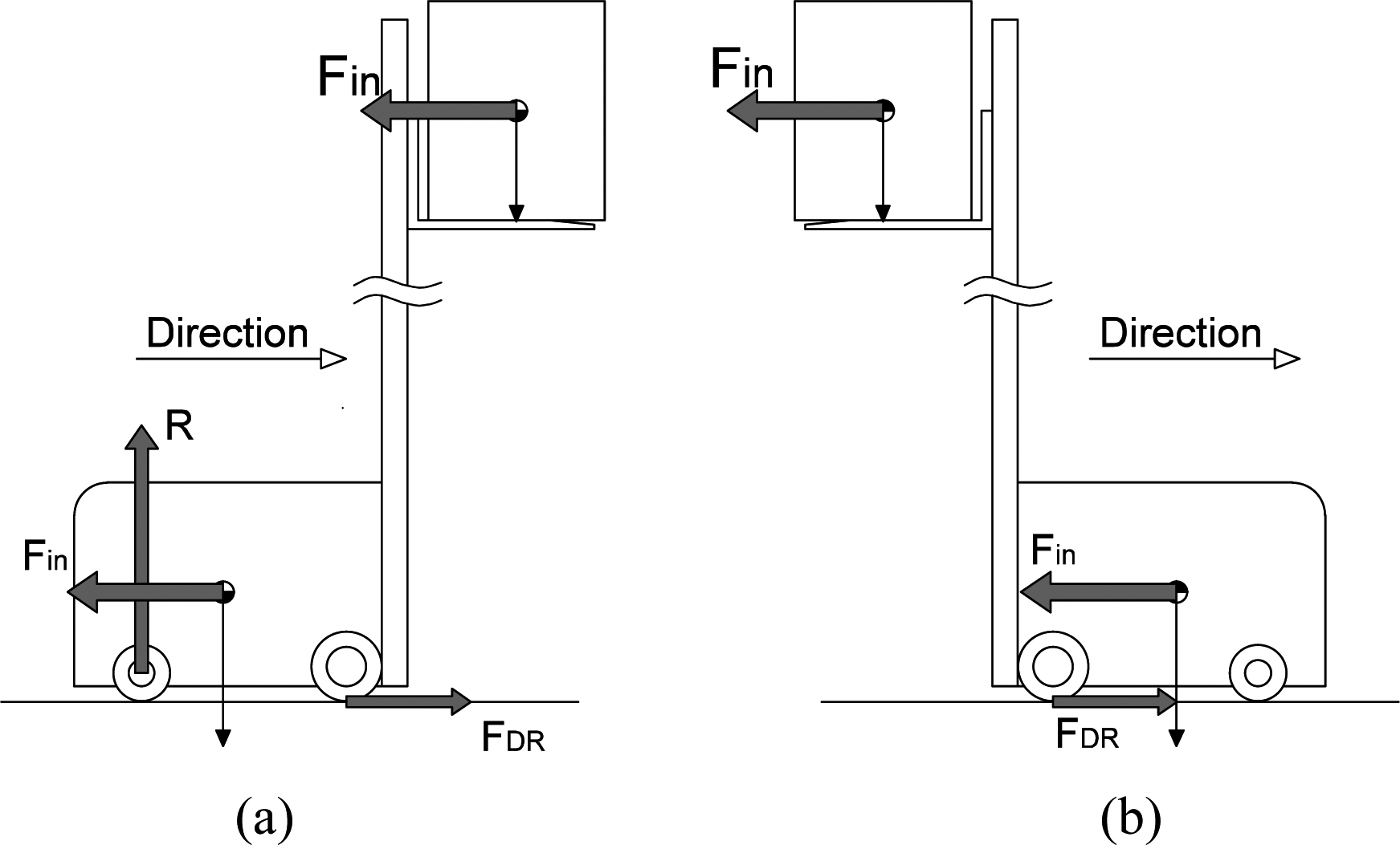
Forklift model and its main dimensions.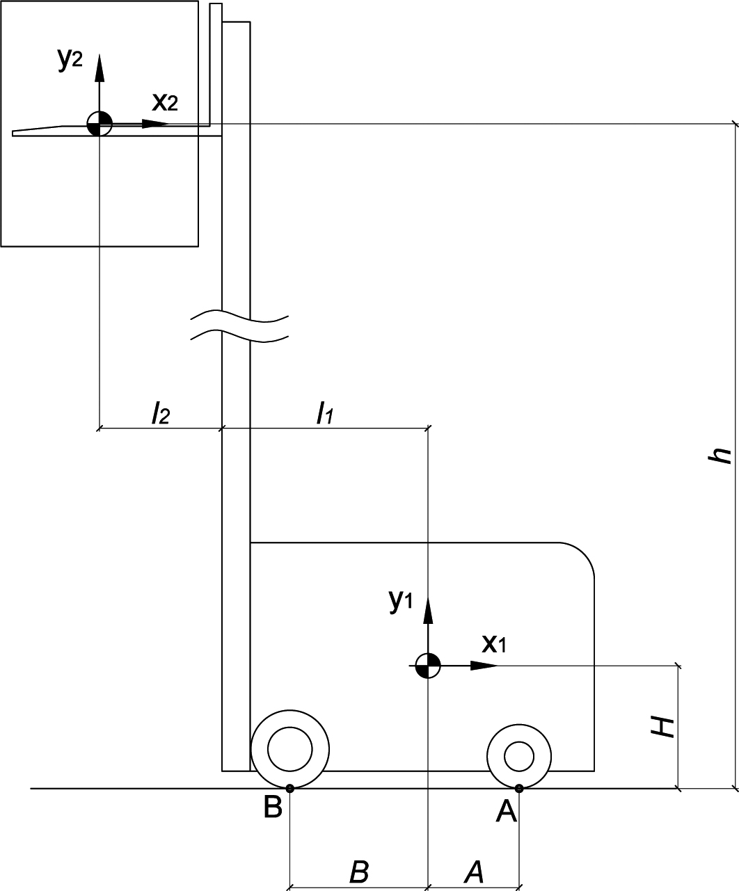
During the braking process the situation is just the opposite. If it is a front load forklift, the inertia forces can cause the truck to tip-over, while if it is a rear load forklift, the torque produced by the inertia forces are compensated with the reaction in the caster wheel.
Model description
The counterbalance forklift simulated is a rear load forklift, as described in Section 2. With this configuration, the vehicle is unstable when accelerating and stable during the braking process. This is considered an important advantage, as acceleration can be controlled, whereas deceleration should not be limited in case an emergency braking occurs. Acceleration stability is achieved with an appropriate stability controller, as explained in this paper.
In order to study the dynamic behavior of the forklift under any load condition, and to understand the related problematic, a bidimensional model is developed. The aim of this model is to obtain analytical expressions for the stability analysis of the system.
In this model, the input is the driving force, and the outputs are the displacements of the center of mass, the pitch angle and their corresponding velocities.
The model has two components: the forklift body and the load. The whole system is considered as a unique body, with the vertical load position
The system has its center of mass located at point G as shown in Fig. 3.
If we consider an inertial frame at
The dynamic equations are obtained by establishing the equilibrium of forces and momentum with respect to the center of mass.
The forces considered, shown in Fig. 4, correspond to the vertical tires reactions with the ground,
Centre of mass and dimensions associated.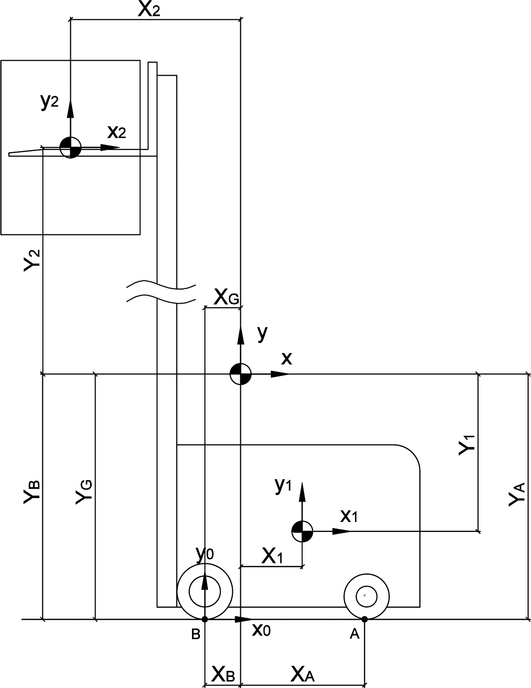
Applied forces.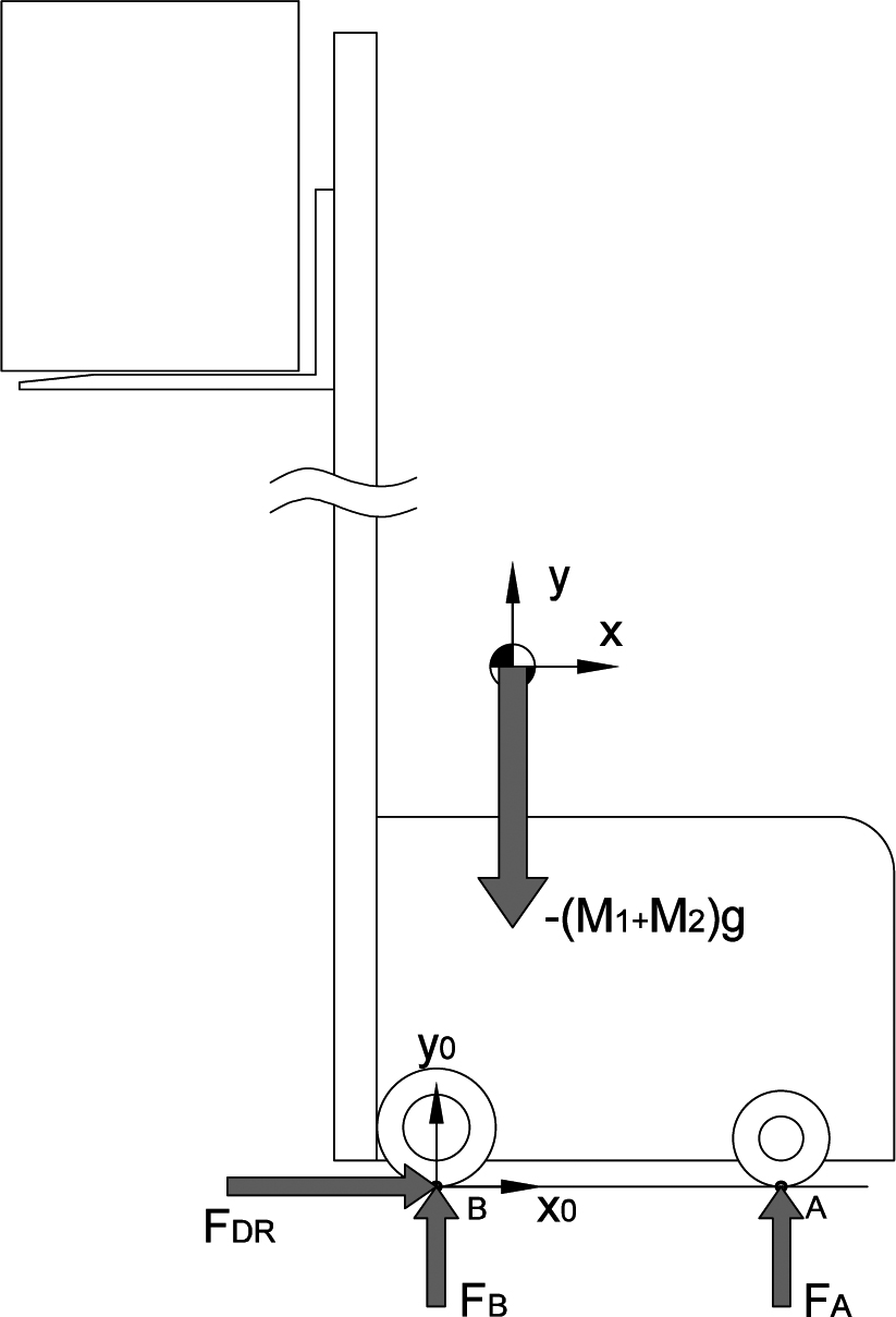
Tires are modelled as a set of two vertical spring-dampers in parallel, by means of the following expressions:
And their related forces are:
If we define the state variables as:
Then, the system equations are written in the form of Eq. (5):
resulting
where
In these equations
Equation (6) is a set of six nonlinear equations. Their nonlinear behavior is due to two facts.
On the one hand, equations are nonlinear because of the trigonometric functions that appear.
But on the other hand, system is also nonlinear due to the behavior of the vertical tire forces
The tires only work under compression, so for these forces, their value is 0 when they are in traction i.e. they are not in contact with the ground, as shown in Fig. 5. This is a key point in the stability analysis.
In order to study and understand the system behavior and its stability, Eq. (6) must be linearized. The resulting equations are Eq. (8)
Then considering
Nonlinear vertical behavior for the tires.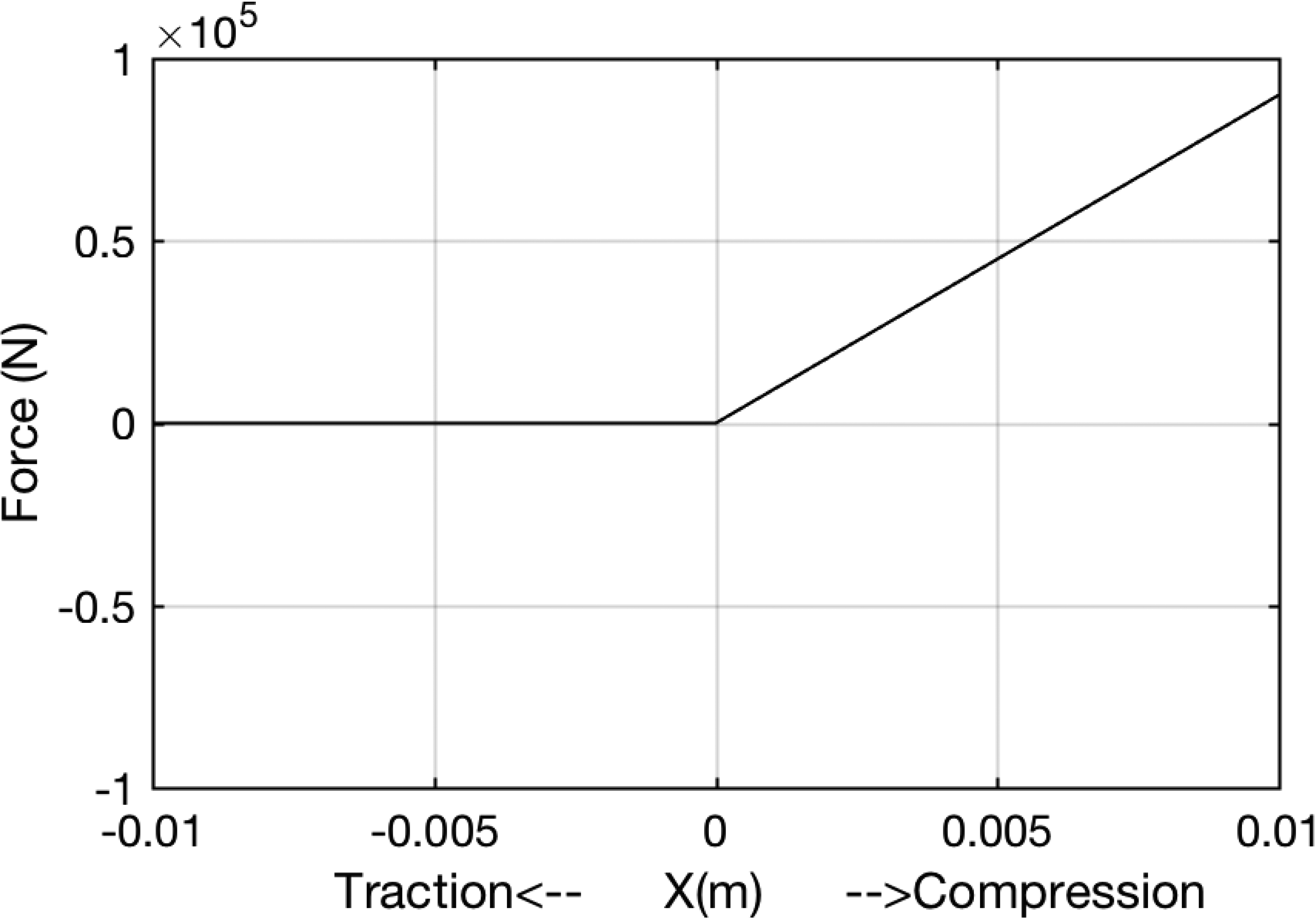
Poles for different load height with 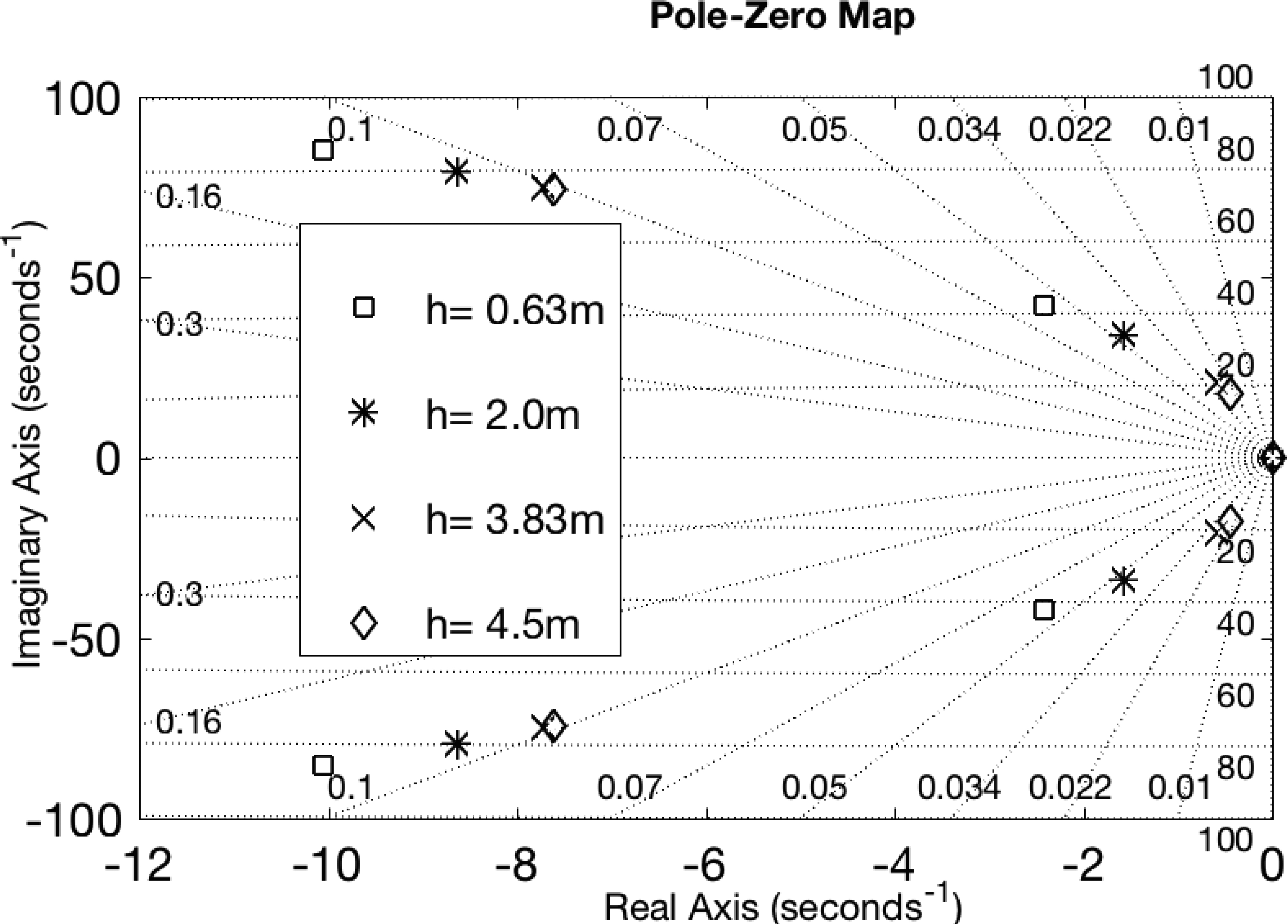
Transfer function U/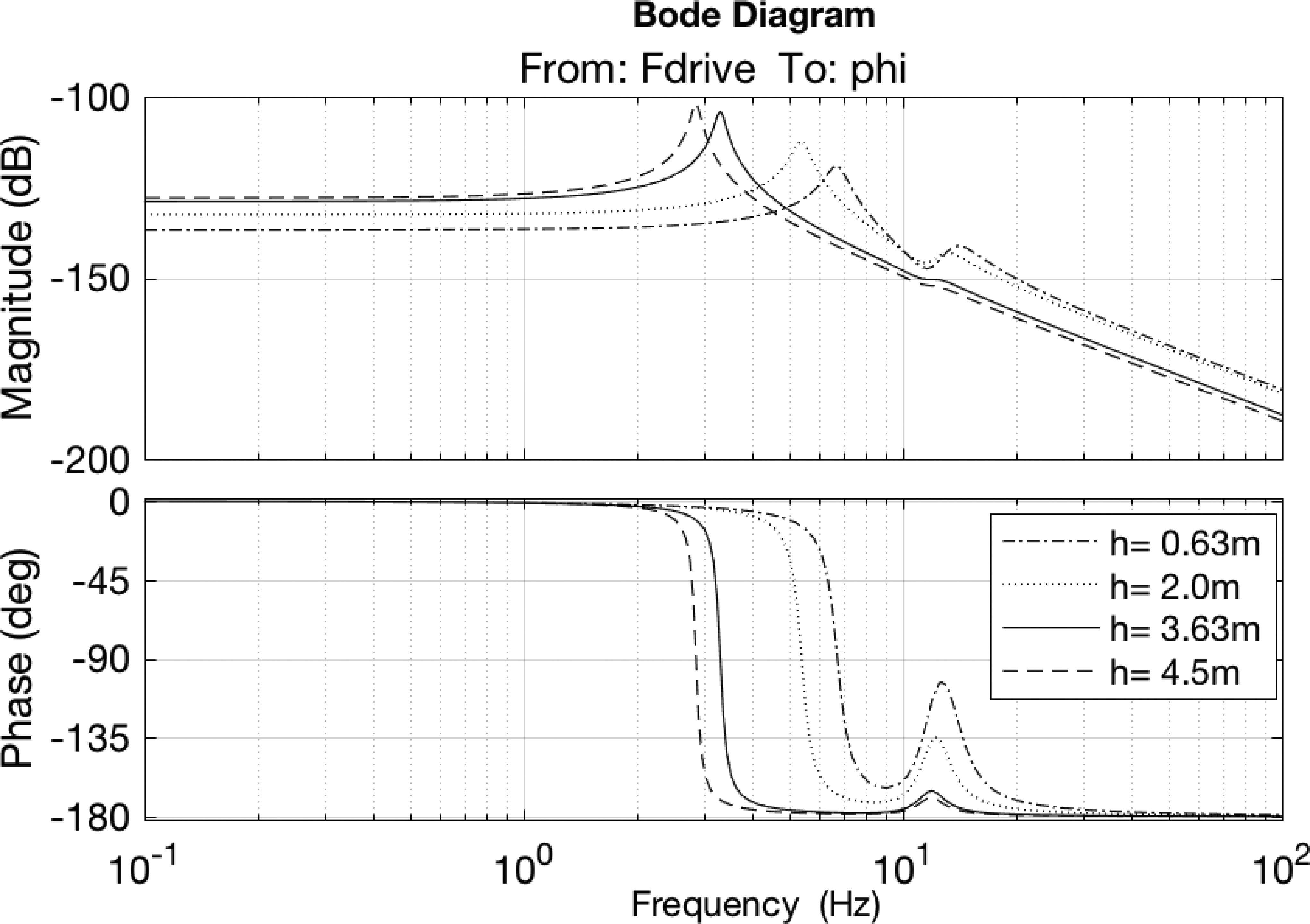
The state-space equations become in the form of:
with,
being
and
And for the output variables:
being the outputs
If we look to the
Because of the
The
The transfer functions are obtained from these matrixes. The transfer function between
with
and
The undamped system is considered in order to obtain the natural frequencies and the vibration modes. In this case, in the transfer function
being
In Eq. (18), the denominator is a biquadratic equation, that allows to obtain the natural frequencies in an analytic way. Then:
Taking into account the possible solutions of
thus
so, it is concluded that two different natural frequencies exist.
This conclusion is visualized with numerical results, as shown in Figs 6 and 7.
Four different load heights are considered: the lowest working height (0.63 m), an intermediate one (2.0 m), the highest working height (3.83 m), and also another higher (4.5 m). For the static position and with
The transfer function (Fig. 7) shows that the value of
Vibration modes.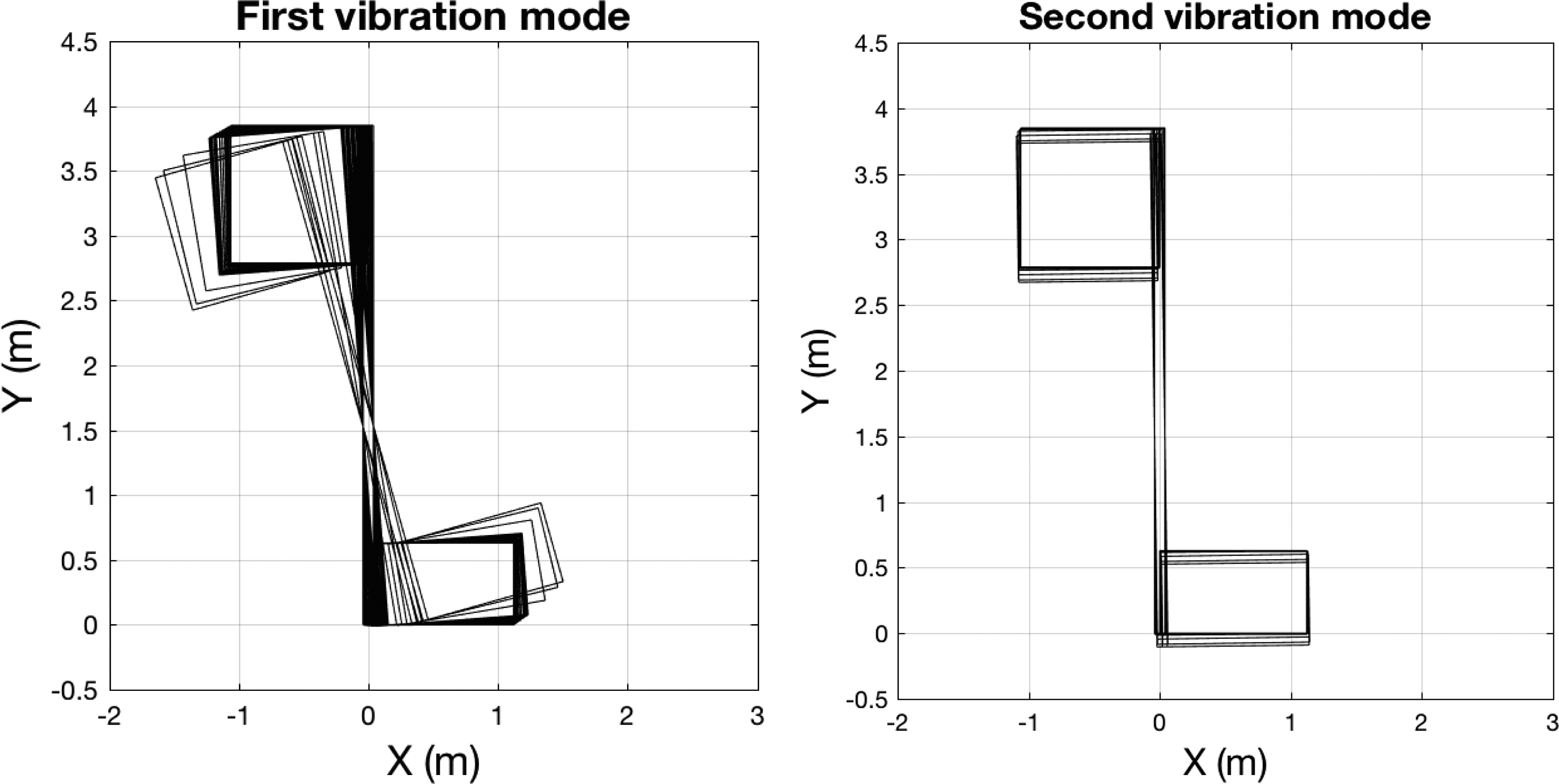
The limit of static equilibrium with
In this case, the
and
The undamped system is considered again in order to obtain the natural frequencies and the vibration modes and the transfer functions is obtained from these matrixes.
Poles for different load height with 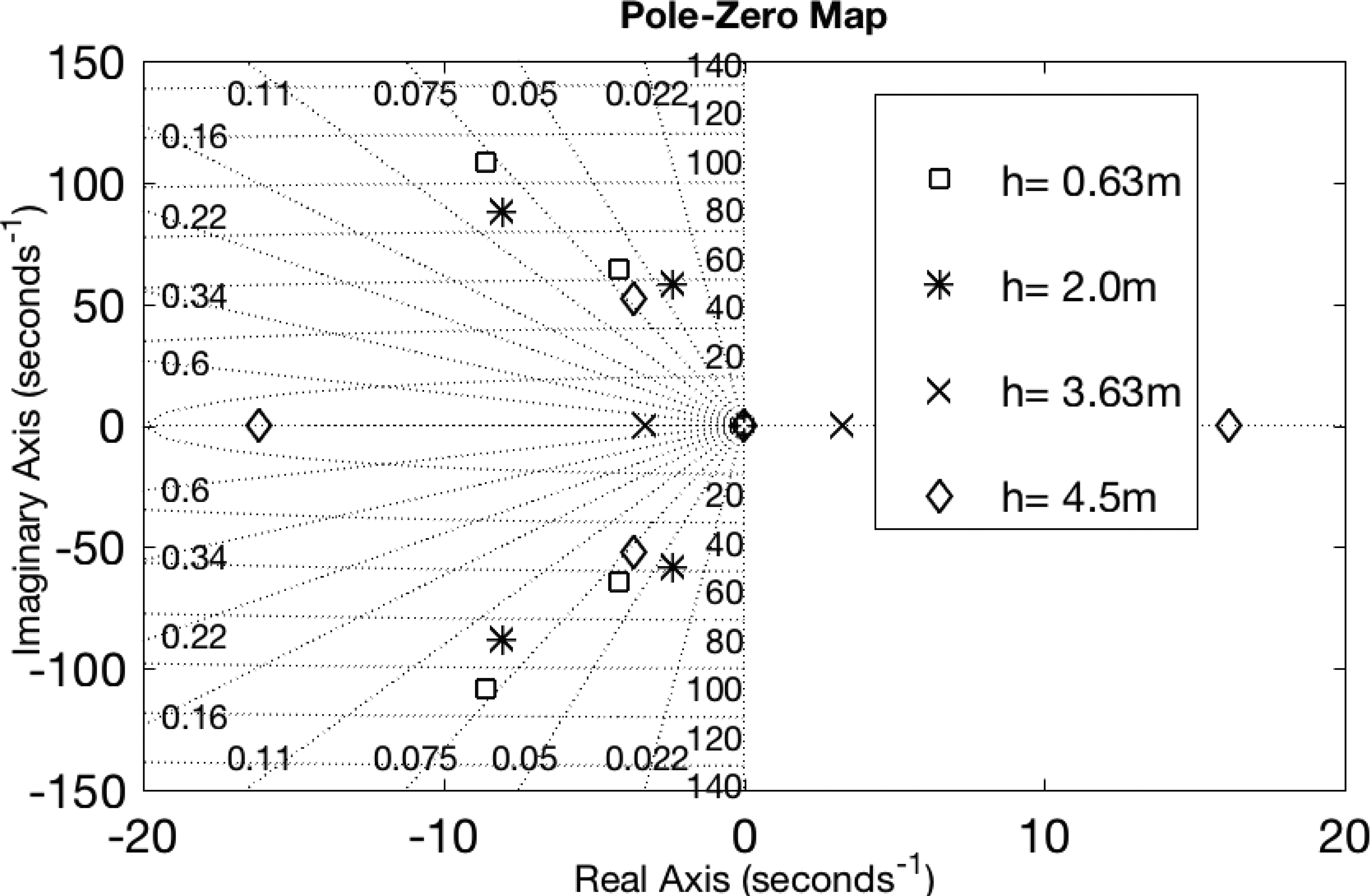
If
The denominator of the transfer function results as:
being
Solving the characteristic polynomial Eq. (27) it is observed that
is always satisfied so, as Eq. (27) is a biquadratic solution, one of its solution is positive, and then an unstable pole appears.
This conclusion is visualized with numerical simulations.
The same four different load heights are considered but the results are quite different. In the first two cases, because of the working load is under the maximum working height, the system is stable, as is seen in Figs 9 and 10, with all the poles with negative real part. But for the third and fourth cases, system becomes unstable having a pole in the right hand of the poles map, as shown in Figs 9 and 10.
Transfer function U/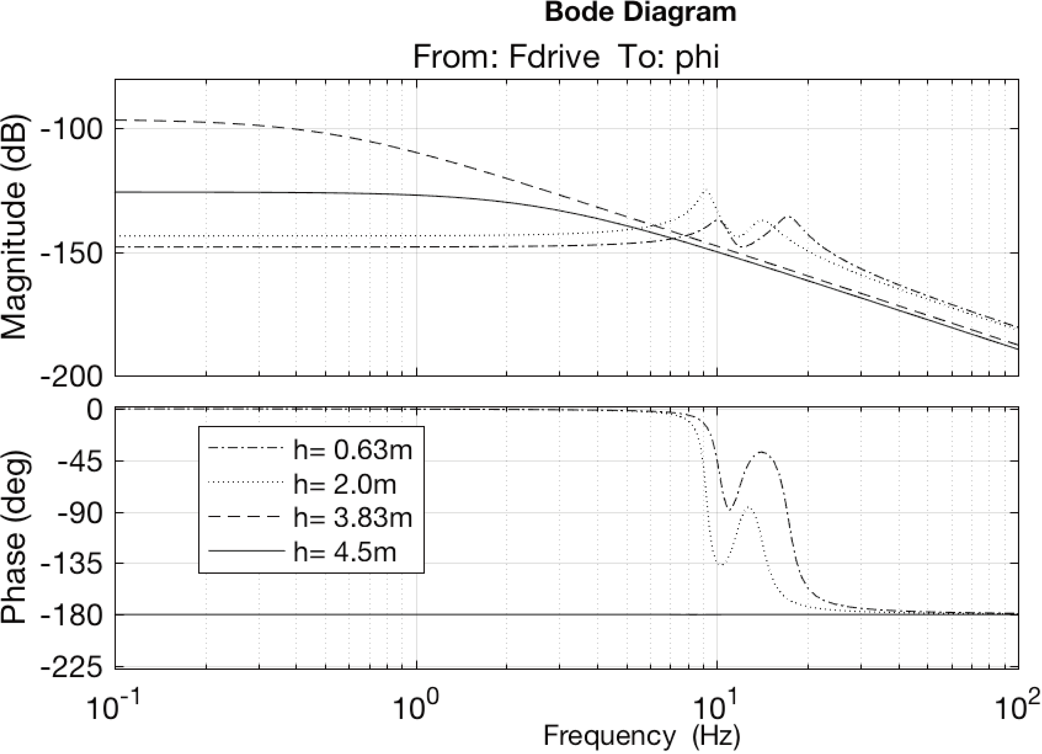
From the previous analysis, it is concluded that, if the forklift pitch angle reaches a limit value, the system becomes unstable, and the tip-over starts.
The open loop simulation is used to determine the dynamic conditions that produce this phenomenon of instability.
The longitudinal tip-over limit is defined as the maximum acceleration that the forklift may achieve without tipping over. In a first approach, this limit is theoretically calculated assuming that the tires are completely rigid.
The equilibrium of moments in
In the limit, the vertical reaction in the front axle,
Substituting Eq. (31) into Eq. (4) and considering
For the parameters considered in the model, the acceleration limit results as
Open loop simulation with acceleration under the limit.
Open loop simulation with acceleration above the limit.
This implies that if the acceleration limit is exceeded and the pitch angle
Figure 11 shows the results of a simulation with a driving force with acceleration under the acceleration limit, observing that the vehicle remains stable.
However, Fig. 12 shows the results of a simulation with a higher traction force, where the acceleration limit is exceeded. Then the system becomes unstable and the forklift overturns.
With the aim of increasing the forklift stability and to guaranty its safety, an anti-tip-over control has been designed considering model predictive control (MPC).
Usually, MPC control predicts future behavior using a linear time-varying (LTV) dynamic model. In many applications, this approach is sufficient for robust controller performance.
But in this case, because of the plant is strongly nonlinear and its characteristics vary dramatically with time when the front wheel loses its contact with the ground, an Adaptive MPC must be used by adapting the prediction model for changing operating conditions, by allowing the model parameters to evolve with time. A terminal constraint has been added in order to guaranty robustness.
The control used presents a MPC controller based on successive linearization of the non-linear vehicle model presented in Eq. (6). This non-linear model is linearized around the current operating point at each time step, and a linear MPC controller is designed for the resulting LTV system.
At each control interval, the adaptive MPC controller updates the plant model and the nominal conditions. Then, for the prediction model, the discrete-time states used can vary with time, which can be obtained from the nonlinear system Eq. (6).
The most frequent approach used in the literature is the explicit Euler method Eq. (33).
This method is easy to implement, but it requires a very small time-step
The implicit Euler method is suitable to keep the error in the result bounded. In this case, to achieve a given accuracy, it takes significantly less computational time to use an implicit method with larger time steps, even taking into account that an equation of the form Eq. (34) needs to be solved at each time step. This equation is solved by the fixed-point iteration method. Implications of the use of each one of this approach will be discussed in the section of simulation results.
The expression of
Taking into account that
where:
The objective of the control system is to track the velocity profile
For the formulation of the MPC a prediction horizon
The notation
Over the prediction horizon
The cost function
subject to:
where
Equation (38d) represents the maximum pitch angle limitation.
Constraint Eq. (38e) corresponds to the maximum allowed driving/braking force. Equation (38f) represents the maximum power constraint.
The way of ensuring stability is to add a terminal constraint which forces the state to take a particular value at the end of the predictive horizon as shown in [18, 19]. The Eq. (38g) corresponds to the terminal constraint used. This constraint is established to enforce that the vertical displacement for the point A is always negative and, consequently, the tip-over is not produced at the end of the predictive horizon. This terminal constraint ensures the stability of the proposed controller, because it ensures that the forklift is always in a stable position.
The function
where:
The full expressions for each component of the cost function are:
being:
For the simulation of the proposed model, a MatLab code has been develope. This code consists of a constrained non-linear optimization problem, that has been developed by using the interface Yalmip [17] and Ipopt [30], solver used for nonlinear optimization problems.
Weights in the cost functions
Weights in the cost functions
Response to different pulses.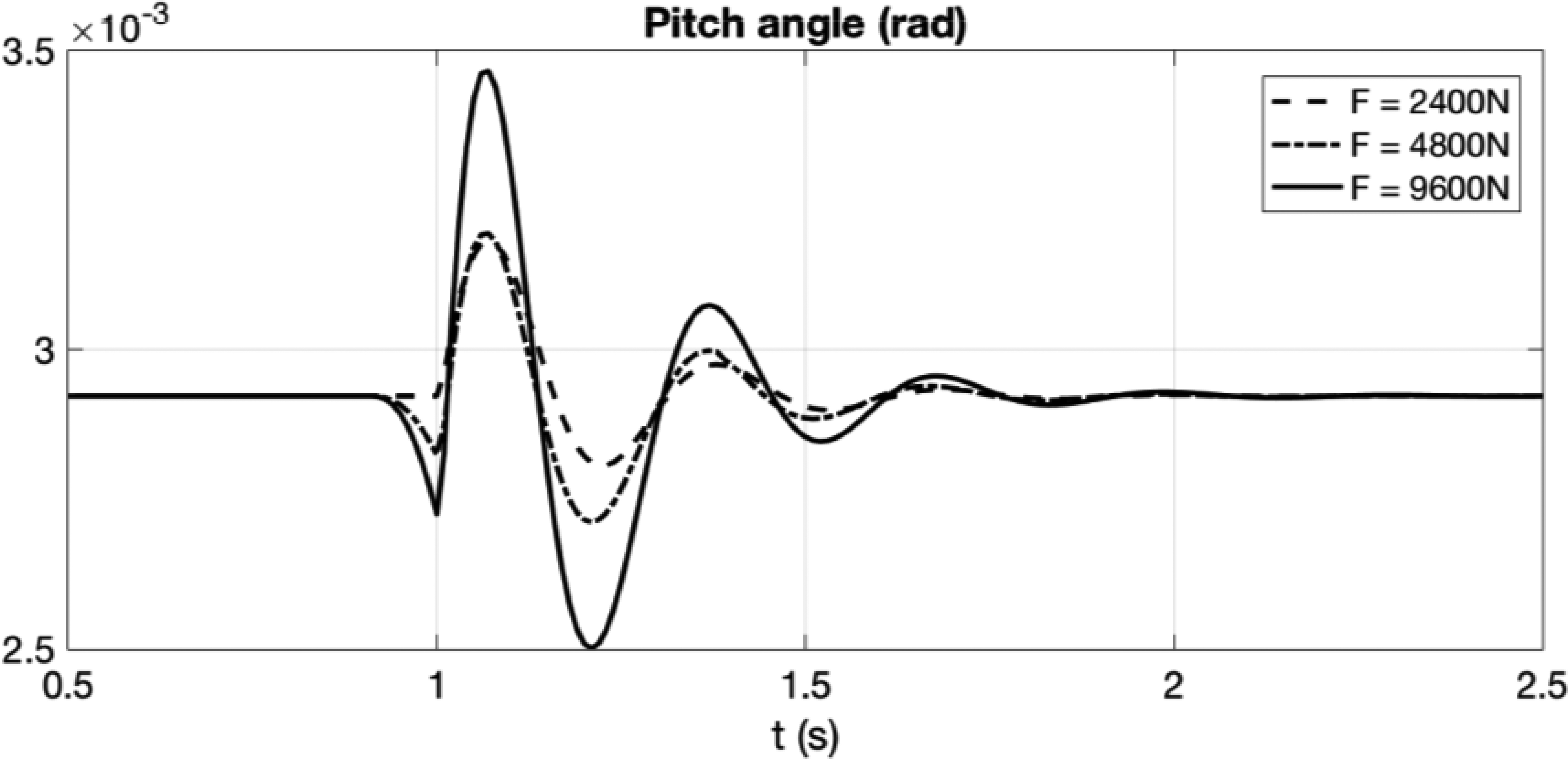
A value of
The predictive horizon
Table 1 lists the corresponding weights in the cost function.
In the simulation, the box constraint on tracking/ braking force is reflected by the maximum driving and braking force
The
First, in order to check the stability, a simulation has been done defining a perturbation by means of a horizontal force defined as a pulse from 1.00 s to 1.02 s with different amplitudes. Figure 13 shows that the system is stable, and it also respects the constraints.
Velocity profile.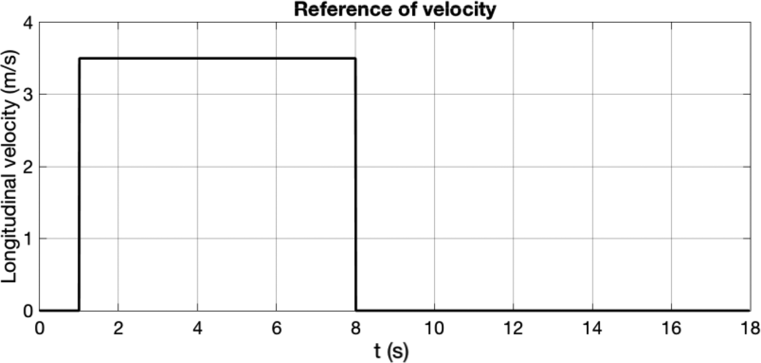
Control input.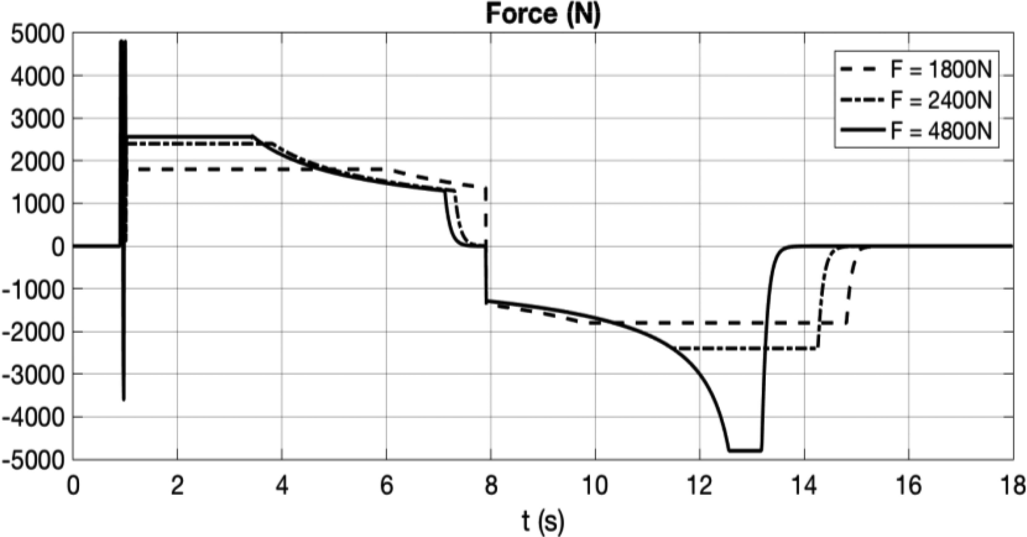
For the simulations, a speed profile is stablished, as shown in Fig. 14 in order to study the system behavior. This speed profile is used to test an acceleration maneuver and, after that, a braking maneuver.
This profile means that when the simulation reaches
Three different cases for
Control input. Detail between 0.5 s and 1.5 s.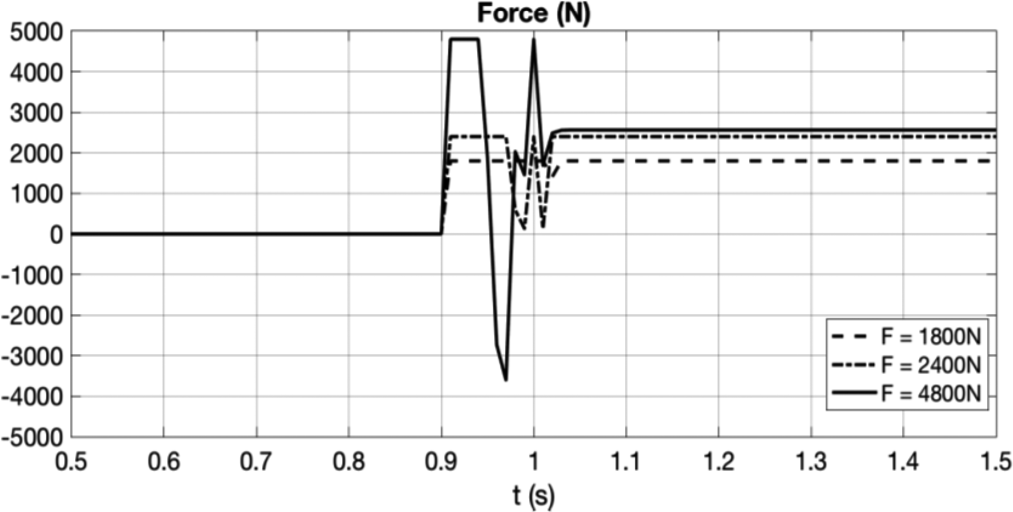
Pitch angle.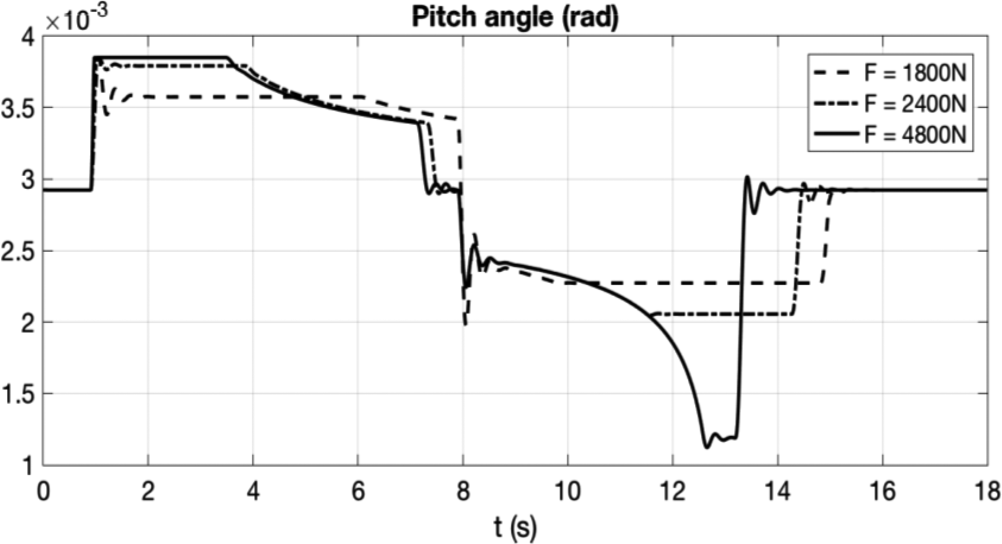
Pitch angle. Detail between 0.5 s and 1.5 s.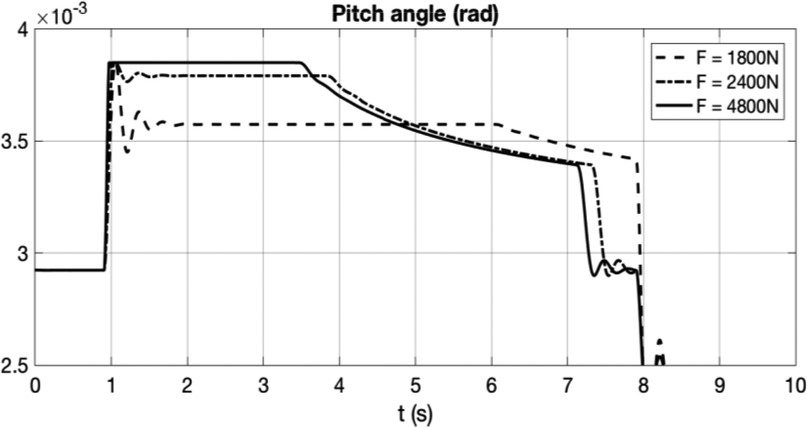
Vertical displacement for the wheels.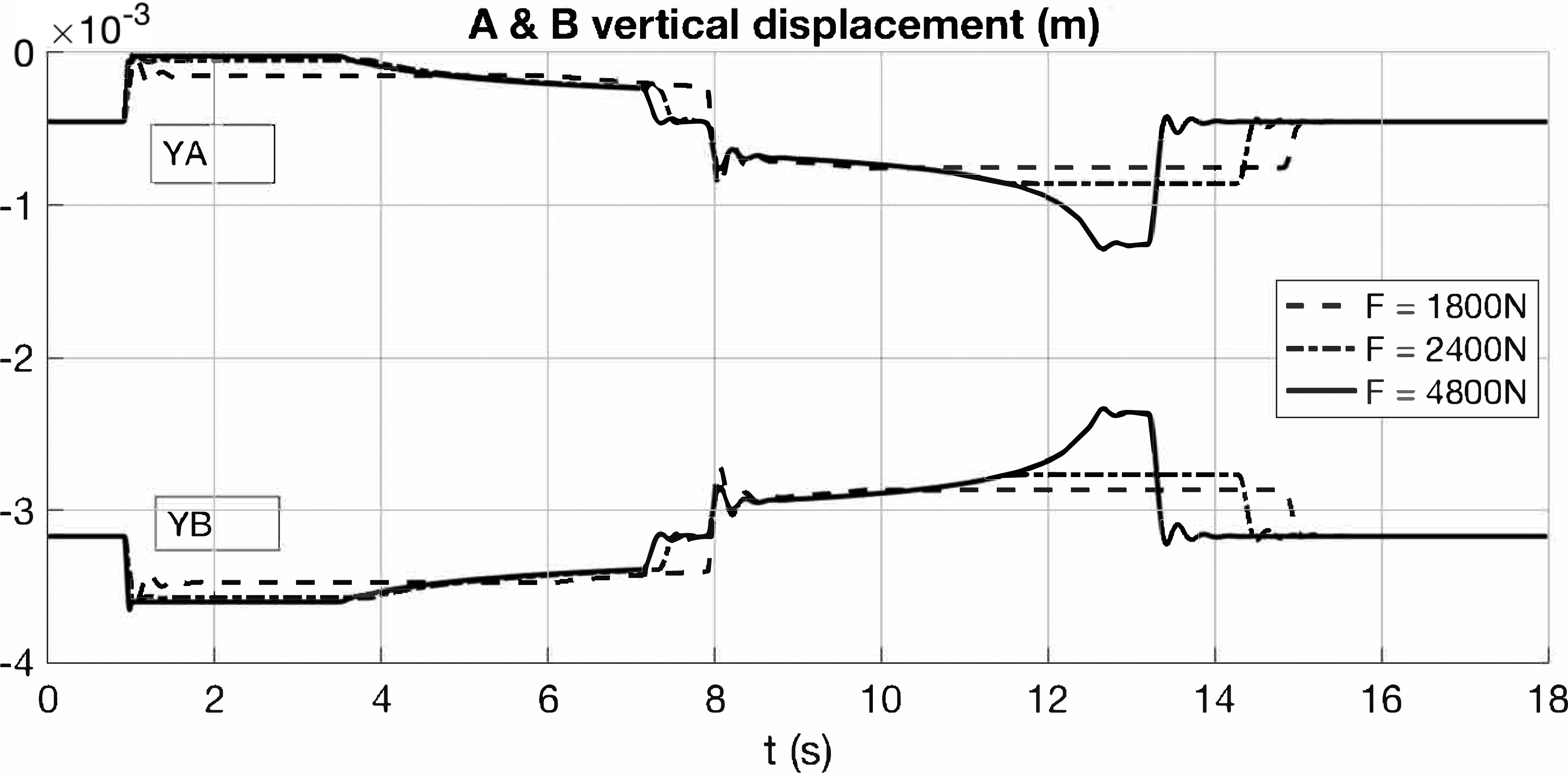
In the second one,
And in the third case,
Figures 15 to 21 show the results for these simulations. In these figures, several variables are represented, including simultaneously in the same plot the results for each
Figures 15 to 18 represent the control input (driving/braking force) and the pitch angle. In the first part of the simulation, when the vehicle accelerates, it is observed that for
Velocity obtained.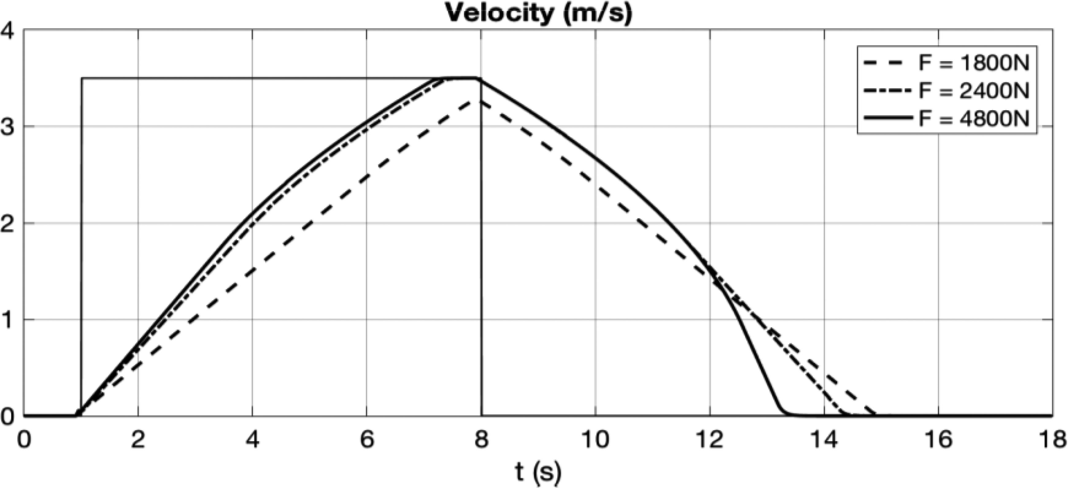
For
On the other hand, the pitch angle (Figs 17 and 18) is not affected in the case of
In the case of
And in the case of
Figure 19 shows the vertical displacements
The stability control imposes that
From an operational point of view, Figs 20 and 21 must be analyzed.
Figure 20 shows the velocity followed in each simulation, showing that for
Figure 20 shows that, in the acceleration phase, for the cases of
But in the braking phase, significant differences appear, because in this case, the vehicle does not have stability problems, and the braking force is not limited.
So, as a conclusion, the stability control improves the operation of the forklift because of it uses the maximum limit force without stability problems when accelerating and it uses the maximum available force when braking, being the total time to carry out the whole maneuver lower for higher driving/brakingforces, as shown in Fig. 21.
Dynamic scaling of the prototype
As mentioned in the introduction, a scaled prototype has been built in order to experimentally validate the control.
Displacement followed.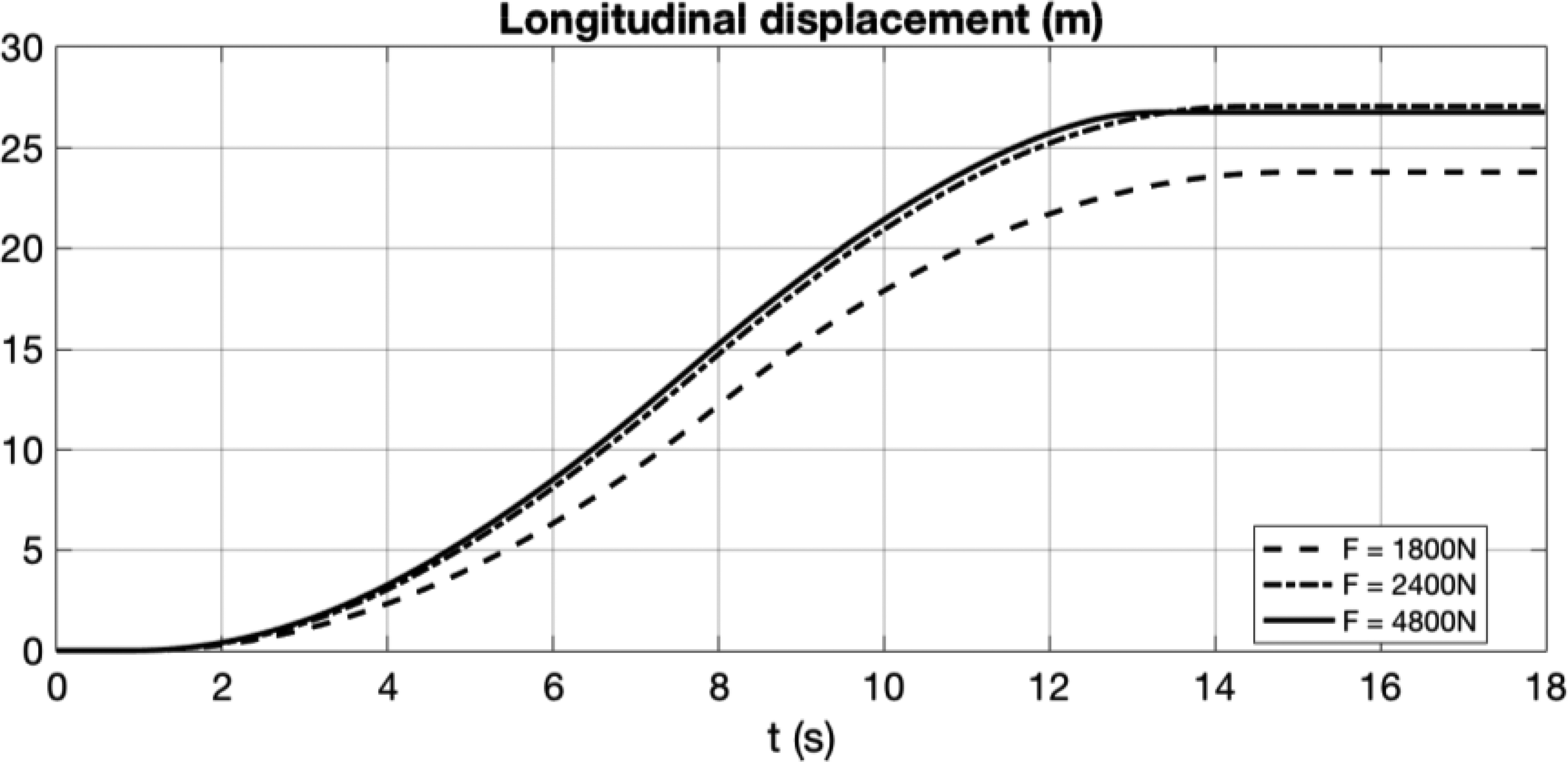
Because of the size and dynamic properties of the prototype are not the same as the properties of the real vehicle, equivalence between both, the real model and the scaled prototype, must be established.
In the literature, different methodologies are proposed for choosing the scaling criteria. [2] includes four of the most common scaling criteria, compared in terms of scaling factors on different physical parameters as a function of the chosen geometrical reduction factor
These assumptions are demonstrated in this case. From Eq. (32), where the longitudinal tip-over limit is calculated, an important conclusion is drawn: if all the magnitudes of longitude are multiplied by a factor
In the same way, the traction force is altered by the masses factor, as shown in Eq. (45). This allows the motors to be much smaller than the real ones.
Therefore, only two different parameters are used as scaling factor for dimensions and masses, respectively, and the longitudinal tip-over limit still remains unaltered in 0.695 m/s
Final prototype.
A first scaled prototype for the forklift was presented [5]. In the prototype, all the electronic components have been chosen so they can validate the control strategy based on the pitch angle. In practice, the sensors that the prototype implements are the following:
BeagleBone Black microprocessor. USB Wi-Fi adapter with 4” antenna. Stepper motors with 400 steps/rev and 68 oz.in Two stepper motor drivers A4988. Accelerometer-gyroscope InvenSense MPU-6050 .
The complete prototype is presented in Fig. 22.
Figure 22 shows the electronic components inside the prototype, and the final appearance of the prototype.
Acceleration for 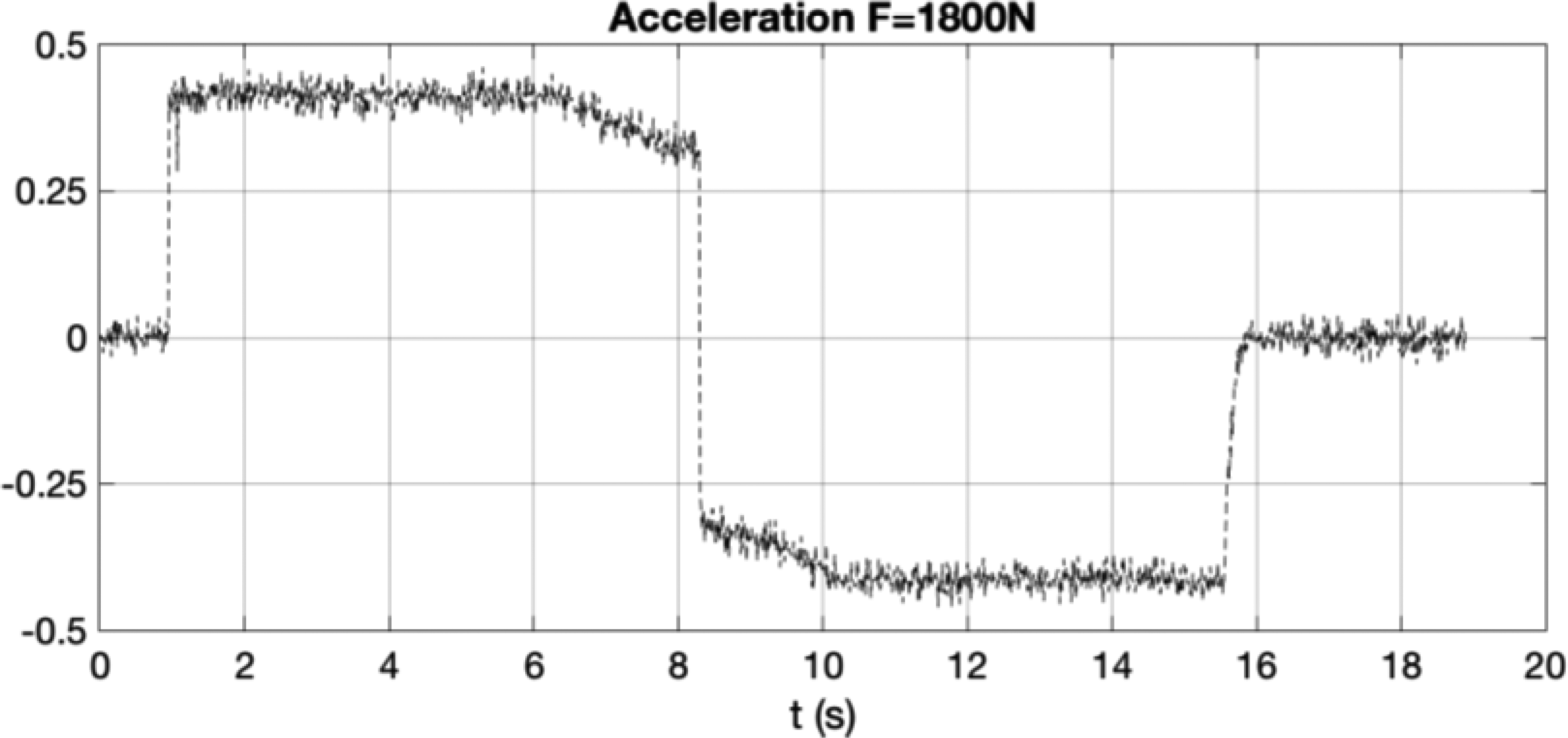
Pitch angle for 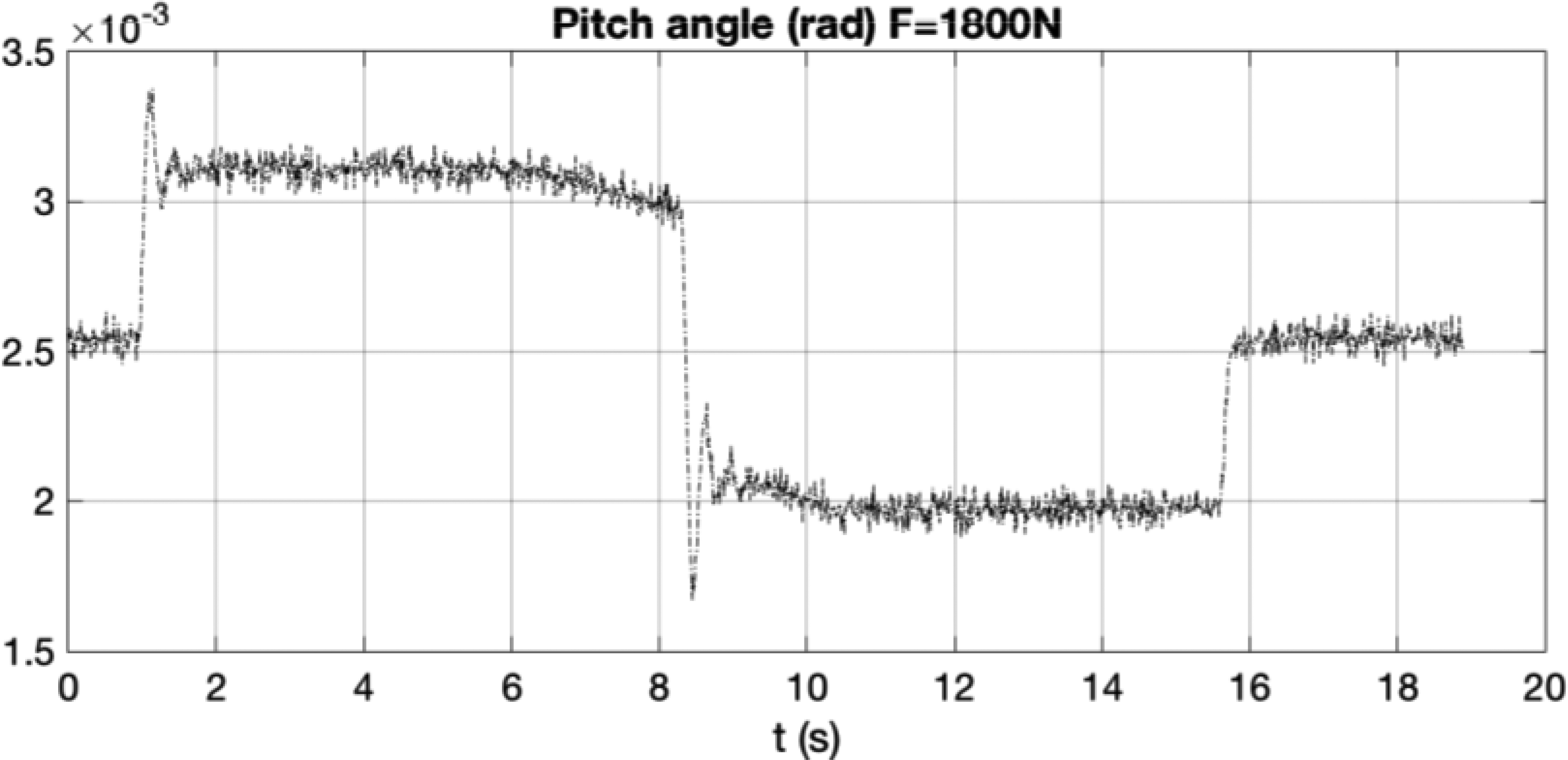
Acceleration for 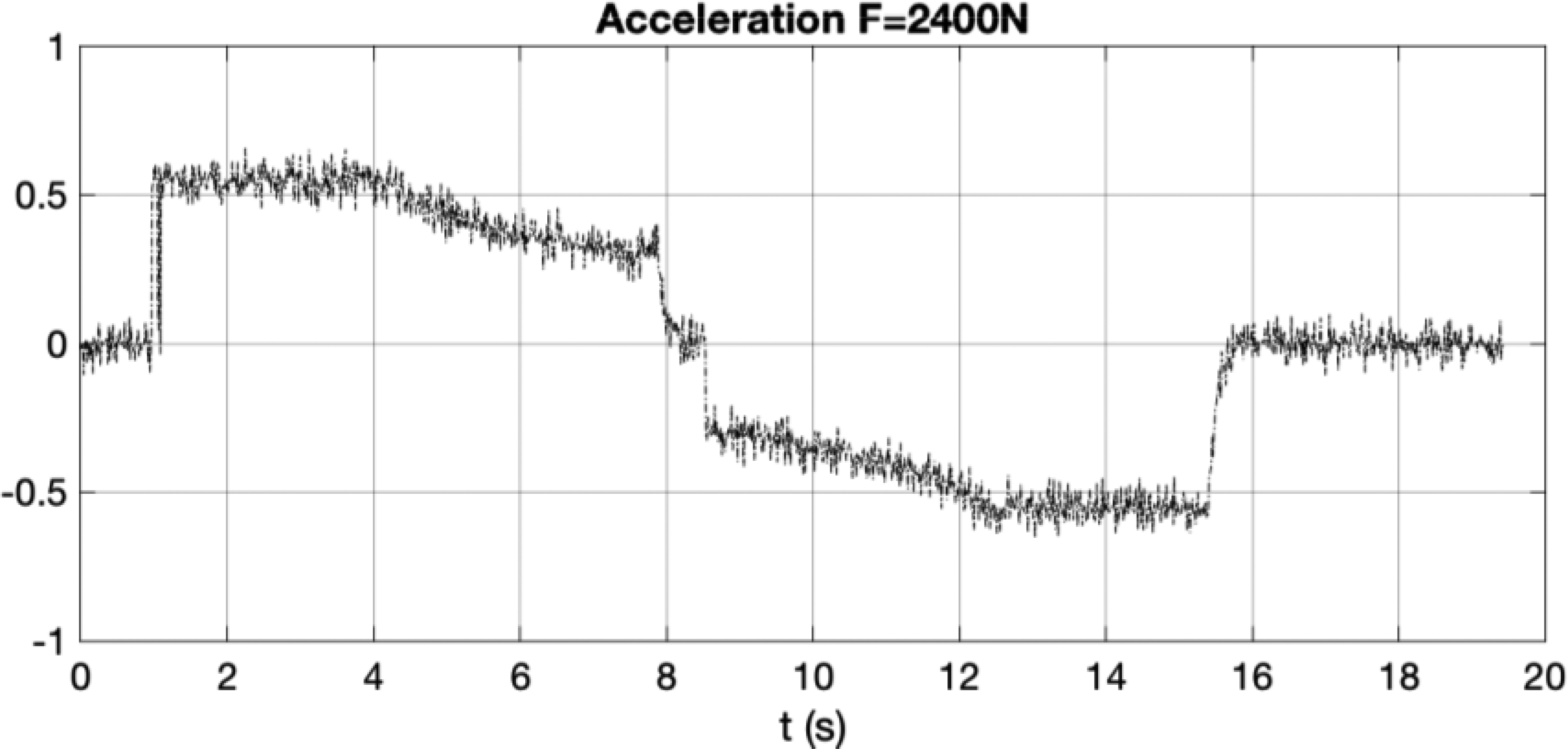
The same control strategy followed previously in the theoretical model is implemented in the scaled prototype and one experiment is carried out with the prototype in order to validate the simulations.
The experiment consists in the same maneuver that the one used in the simulations.
The experiment was conducted with two scaled forces of 0.36 and 0.48, corresponding to the original forces of 1800 N and 2400 N.
In the first case, the anti-tip-over control do not need to work, because of the maximum applied force is below
The second case corresponds to a scaled force of 0.48, equivalent to 2400 N. Figure 25 shows the measured acceleration and Fig. 26 shows the pitch angle obtained in this case.
The limit obtained experimentally was 0.6 m/s
Pitch angle for 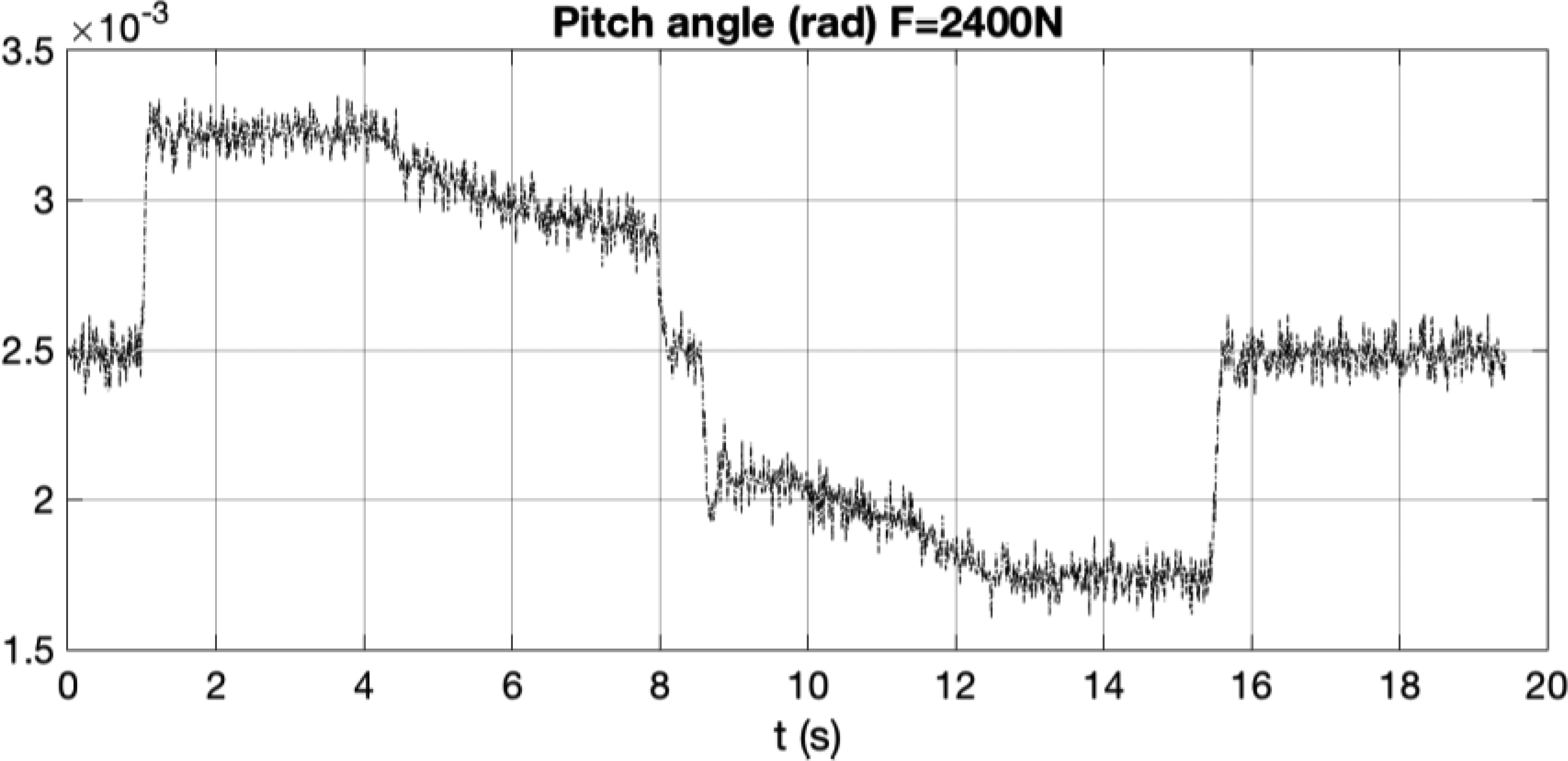
The results presented in Figs 25 and 26 show a similar behavior to the simulations.
The experiments demonstrate that the control strategy is perfectly feasible, and also that it satisfies all the requirements: it achieves the maximum acceleration possible under any load condition and it is stable under external disturbances. The result is a faster and safer forklift as the tip-over risk decrease drastically.
This paper presents the design of an anti-tip-over control applied to a counterbalance forklift, a highly unstable vehicle, mainly in relation with its pith angle.
With this new concept in the field of forklifts, stability is significantly improved, since this control not only decreases the risk of accidents, but also reduces the transportation times and consequently the operational costs.
First, an analytical study has been developed in order to analyze the characteristics of this kind of vehicles and their stability problems. As a result of this analytical study, the conditions for stability are obtained showing when this type of vehicle becomes instable.
After that, a MPC controller is designed and implemented. This kind of control has been successfully used in autonomous vehicles, being the objective of this paper to demonstrate how feasible it is in this particular vehicle.
Several simulations and test are carried out. The results are very satisfactory, showing that the forklift is able to maintain its stability under conditions that a vehicle without control would be unstable. In particular, in acceleration, the vehicle is able to avoid the tip-over by controlling the pitch angle, but when braking, the forklift is able to use all the braking capacity. Thus, as a conclusion, the vehicle with the controller is able to carry out acceleration and braking manoeuvers in a more quick and safe way.
In order to validate the control strategy and ensure that the controller is feasible, an innovative procedure for validation using a scaled prototype has been developed allowing to detect design problems in a previous stage before to build the real and high cost prototype. Simulation have been replicated with experimental tests obtaining equivalent results.
Hence, and because of all the simulations and test have obtained positive results, it is concluded that the MPC controller, based on the pitch angle regulation, increases safety, significantly reduces the transportation times, and consequently reduces the operational costs, being thus especially advantageous.
Footnotes
Appendix
The main parameters of the model are:
Parameter values
| Parameter | Value |
|---|---|
|
|
2.650 kg |
|
|
1.050 kg |
|
|
491 mm |
|
|
439 mm |
|
|
491 mm |
|
|
630 mm |
|
|
630 mm |
|
|
3.580 mm |
|
|
160 mm |
|
|
1 10 N/m |
|
|
1 10 N s/m |
|
|
0.8 |
| Maximum power per motor | 4.5 kW |