Heuristic ensemble for unsupervised detection of multiple types of concept drift in data stream classification

Abstract

Real-world data stream classification often deals with multiple types of concept drift, categorized by change characteristics such as speed, distribution, and severity. When labels are unavailable, traditional concept drift detection algorithms, used in stream classification frameworks, are often focused on only one type of concept drift. To overcome the limitations of traditional detection algorithms, this study proposed a Heuristic Ensemble Framework for Drift Detection (HEFDD). HEFDD aims to detect all types of concept drift by employing an ensemble of selected concept drift detection algorithms, each capable of detecting at least one type of concept drift. Experimental results show HEFDD provides significant improvement based on the $z$ -score test when comparing detection accuracy with state-of-the-art individual algorithms. At the same time, HEFDD is able to reduce false alarms generated by individual concept drift detection algorithms.

Keywords

Concept drift ensemble data stream mining

1. Introduction

Data stream classification has become a very important topic of study as the amount of digital data increases rapidly. Traditional classification problems consist of learning an underlying data distribution, called concept, among several data classes from a static dataset. The dataset is assumed to contain all information needed for training classifiers. This static model is insufficient when applying to real-world data stream classification applications [1, 32]. Many of those applications, such as online sentiment analysis, intrusion detection, and fraud detection, have dynamic data stream where changes in data might reduce quality of a classification model. For example, a new type of credit card fraud can appear that tries to circumvent existing fraud detection models in place. These changes in data streams, named concept drift [3, 22, 26], often affect the underlying data distribution and reduce the performance of existing classifiers.

Designing high performance concept drift detection approach is not a trivial matter. There is often a trade-off between cost efficiency and performance among frameworks [34, 25]. Relative high performance can be achieved with labeled streaming data. But, labeling or even only partial labeling an unlabeled, high-volume, indefinite-sized data stream using human experts may involve high cost [34]. The scale and velocity of modern day data applications makes such dependence on labeled data a practical and economic limitation. Streaming data applications need to be able to operate and detect drifts from unlabeled, or at most sparsely labeled data, to be of any real use. Unlabeled data used for concept drift detection eliminates the cost of human intervention [4, 5]. This however, often results in lowered detection performance since concept drifts take on various forms and are often unpredictable [10]. Two examples of changes in unlabeled data stream are shown in Fig. 1. In Fig. 1a, the data stream seemingly undergoes no change when labels information is absent. Once labels are obtained in Fig. 1b, it is clear that drift in data has rotated initial linear classification model from horizontal to vertical. In Fig. 1c, a new data region appeared outside of existing data distribution, thus signaling a potential concept drift. After obtaining labels in Fig. 1d, it turns out the new region is not a source of concept drift because the classification model is not affected. In this case, the detection of concept drift with unlabeled data will generate a false positive. It results in increased sensitivity to change, and a large number of generated false alarms. False alarms in drift detection make the algorithm behave overly sensitive, lead to wasted training effort, and reduce confidence in a streaming data classification model [23].

Figure 1.

Detecting various types of concept drift is difficult without label.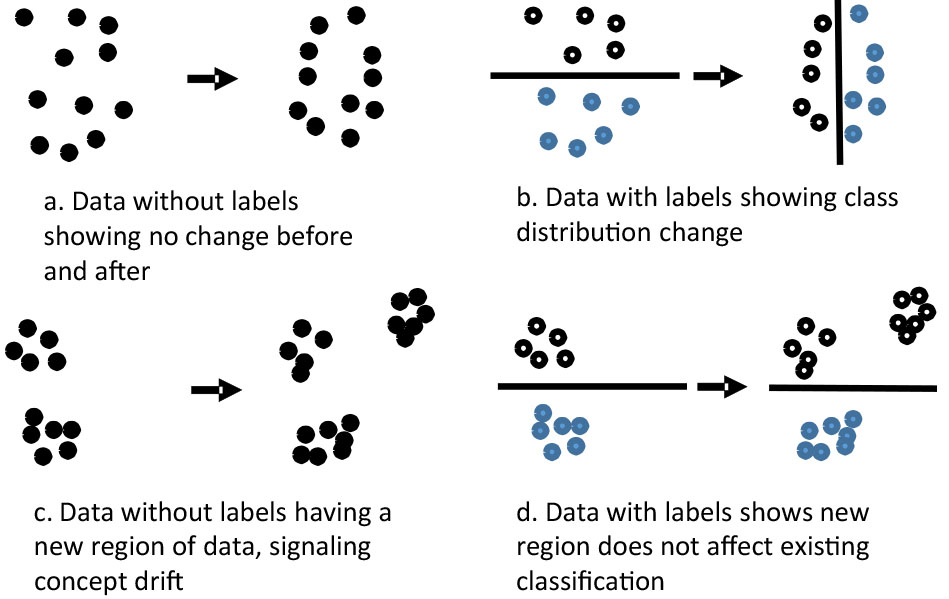

Majority of existing concept drift detection algorithms, while performing well with labeled data, may show limitations when presented with unlabeled data. The complex nature of concept drift brings many more types of drift other than the presence of distribution change shown in Fig. 1 [20, 14]. A drift can occur abruptly, or slowly over time [8]. Drifts can occur repeatedly, or occur periodically [33]. Algorithms that focus on one aspect of concept drift characteristics will inevitably fail when such characteristic does not appear in a particular drift. For instance, an algorithm that focuses on detecting new data distribution will be able to detect change in Fig. 1c most of the time even without class labels. However, such algorithm might fail at detection concept drift in Fig. 1a, because the characteristic of change in distribution required by the algorithm does not occur. Another algorithm, such as SVM Margin [6], might be able to detect changes in Fig. 1a but not in Fig. 1c. A better strategy is therefore to combine the strength of both algorithm so that both types of concept drift scenario can be detected.

Table 1

Overview of concept drift types with constant features and classes

Detection scope	Criteria	Type
Single drift	Speed	Sudden/abrupt
(drift without memory)		gradual
		Incremental
	Distribution	Fixed space
		non-fixed space
Drift sequence	Recurrence	Recurrent
(drift with memory)		non-recurrent
	Time interval	Periodic
		irregular

This paper proposes Heuristic Ensemble Framework for Drift Detection (HEFDD) in streaming data. HEFDD applies the theory of ensemble to bring together multiple algorithms, each performing best at detecting some, but not all, types of concept drifts. A novel hierarchical voting mechanism ensures that different types of concept drift can be detected, even when global voting does not produce a majority. Such voting mechanism also helps to reduce the number of false alarms raised by individual detection algorithms. Main contributions of this paper are:

Formulate a heuristic ensemble framework for unlabeled detection of various types of concept drift.

Outline criteria of algorithm selection for implementing the ensemble

Experimentally show the advantage of the ensemble approach compared to variety of single detection algorithm.

The remaining parts of the paper is organized as the following. Our taxonomy of drift types will be explained in Section 2. Review of existing concept drift detection algorithms will be presented in Section 3. The proposed ensemble approach EFDD is formulated in Section 4, while the experimental result are presented in Section 5. Section 6 concludes the study, followed by references

Figure 2.

Sudden, Incremental and Gradual Drift classified by speed of change.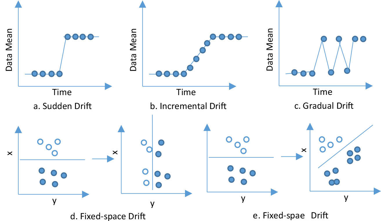

2. Concept drift types

Our analysis of concept drift starts with the assumption that the feature space and class assignment of a stream are fixed, meaning no new feature will appear and no new class will be designated. Table 1 shows the overview of concept drift types. The types are compiled from studies done by Minku et al. [19, 20], Gama et al. [8], Webb et al. [33] and Khamassi et al. [13, 14]. The left most column shows two different scopes of drift detection. Single Drift means that the detection process only looks for the current drift. It does not take previous drifts into consideration, or drift detection assumed to be without memory. Drift Sequence means that detection process takes multiple historical drifts up to the current drifts into account, which represents drift detection approaches with memory. The middle column in Table 1 shows the additional criteria of categorization. For Single Drift, the speed of change categorize drifts based on how fast the classification boundary of underlying model changes. Sudden drifts occur immediately, usually within one time step while Gradual and Incremental drifts occur slowly, spanning multiple time steps. The distribution of change categorize drifts based on whether the drift is happening within the same region of existing features’ space. If change is happening within the same region, these drifts are called Fixed Space drift. Otherwise, they are called Non-fixed Space drift. For Drift Sequence, two criteria of categorization are considered: Recurrence and Time Interval between drifts. Recurrence categorize a series of drifts into Recurrent, where a single drift in the series repeats itself, and Non-recurrent, where previous drifts do not occur again in the future. Finally, time Interval describes whether a series of drifts occurs in periodically or with an irregular interval. This study focuses on detecting single concept drift, whose types will be discussed in detail below.

Figure 3.

Illustration of combination between speed and distribution of change.

2.1 Criteria for classifying concept drift

Two criteria are used to classify drift in this study: speed and distribution. The speed of change is measured by the number of time steps needed for the drift to complete [19]. A time step can be the arrival of a single sample, a group of samples, or a fixed time interval. The less time steps it takes for the concept to complete, the faster the drift is. If the drift is completed in one time step, it is called a Sudden or an Abrupt Drift. An example of data stream with sudden drift is humidity sensor’s sudden increase in value when it rains. If the drift takes more than one time step, it is either an Incremental Drift or a Gradual Drift. The difference between Incremental and Gradual drift is whether there are intermediate samples between the initial and final stage of concept drift. Gradual and incremental drift can occur within changes in demographic data of a city. Visually, all three types of drift categorized by speed of change is illustrated in Fig. 2a–c. Each dot in Fig. 2a–c represents the current mean value of a chunk of data within a time step of a one-dimensional data stream. The drift shown in Fig. 2a is the Sudden Drift, where the samples abruptly shifts to a higher mean value of the samples. The entire process is complete in one time step. Incremental Drift, shown in Fig. 2b, has mean value of the samples slowly shifting upwards. After 5 time steps the final mean value settles, completing the drift. The data samples that arrived during the 5 time steps have values that are between the initial and final values of the mean. These samples are intermediate samples. When these intermediate samples are absent and the drift is not sudden, then it is a Gradual Drift, shown in Fig. 2c. This drift also takes 5 time steps to complete. However, the data mean change back and forth between the initial and the final, with no intermediate values.

The distribution criterion divides concept drift based on whether there is change in the global data distribution after concept drift is completed. Note that it is the global data distribution since concept drift guarantee changes in single class distribution A Fixed space concept drift means that the global distribution of the data after concept drift remains the same as the beginning of the drift. For instance, Bio-reactor data stream can have bacteria growth condition shifts under different production stages, but the condition remains in a fixed range to keep the population alive. A non-fixed space drift alters the global data distribution during the drift process. Online trending topic data stream is a good example of non-fixed space drift, where a completely new trend can emerge anytime. Visually, these two types of drifts are illustrated in Fig. 2d–e. Each dot represents one data sample of a two-dimensional data set. Fixed space drift is shown in Fig. 2d using two dimensional sample data. The global data distribution remains the same before and after the drift. However, within the global data distribution, single class distributions indeed change, which alters the linear classification model between the two classes. In Fig. 2e, the global distribution along with single class distribution changes after the drift. A new group of samples from the solid circle class appeared outside the initial global distribution. Therefore this is a non-fixed space drift.

2.2 Combinations of drift types by speed and distribution

Since speed and distribution are two independent criteria, the combinations of concept drift types under the two criteria yield six different types of concept drift: Fixed Space Sudden (FSS), fixed space gradual (FSG), fixed space incremental (FSI), non-fixed space sudden (NFSS), non-fixed space gradual (NFSG) and non-fixed space incremental (NFSI). The combinations describe whether a concept drift has global distribution change and how fast the change is at the same time. Figure 3 illustrates two of the combined types: FSS and NFSI.

Fixed space sudden (FSS) drift is illustrated in Fig. 3a. Initially, the linear model between the circle and triangle classes is slanted upwards. Within one time step between time steps 2 and 3, the linear classification model shifts to slating downwards. Although individual class distributions have changed, the global distribution remains the same. Because the drift completes in one time step and the global distribution is fixed, this is a fixed space sudden drift. For non-fixed space incremental drift (NFSI), the illustration is shown in Fig. 3b. Similar to illustration above, the drift takes 3 time steps to complete. The linear classification model changed from upward sloped to downward sloped. In addition to the boundary, the global distribution of data also changed. Different from above is the presence of intermediate data in time step 2 and 3. The circle class slowly shifts its distribution to the lower right corner, rotating the decision boundary slowly in the process. Eventually in step 4 the boundary and data distribution settle, completing the drift.

The reason for combining speed of change and distribution of change into six categories is because current concept drift detection methodologies are with different sensitivities to these six types of concept drift [19, 8, 33]. Some focus on detecting sudden concept drift, while the others focus primarily on detecting non-fixed concept drift. Different emphasis on detection methodologies results in concept drift detection approaches being only suitable to a subset of concept drift types. This aspect of concept drift detection is discussed further in Section 5, where a new technique for multiple types concept drift detection is proposed.

Figure 4.

Basic principle of data distribution based statistical testing.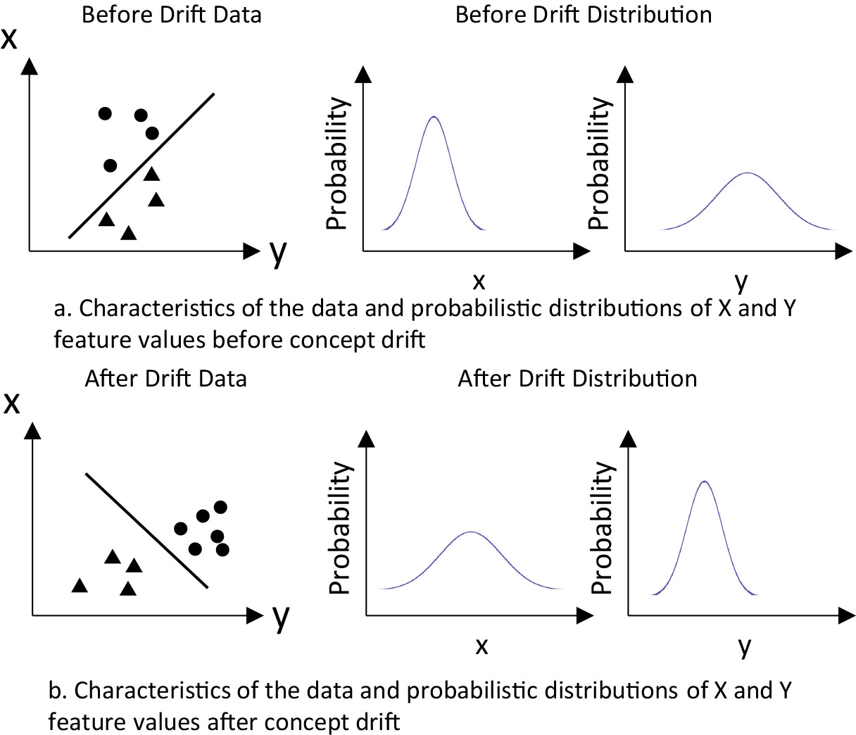

3. Related work

The majority of current state of the art concept drift detection algorithms can be divided into two groups: a) performance based and b) distribution based. Performance based approaches require labeled data because they track the performance of the classification result. Without labels it is difficult to obtain an accurate performance evaluation. Data distribution based approach has the advantage of being able to process both labeled and unlabeled data. When distribution based approach works with labeled data, its detection can be on par with that of performance based approach [6, 25]. When working with unlabeled data, however, distribution based approaches often have limits on what types of concept drift each can detect. This is because most of the techniques are primarily based on assumptions of single type of concept drift detection, while the other types are rarely detected. Since the study focuses on unlabeled concept drift detection, distribution based approaches will be reviewed in detail. Distribution based approaches can be further divided into three groups: a) Statistical test based, b) density based and c) Learning model based. Algorithms in each group employs similar detection techniques, which means they have similar limitations on the types of concept drifts they can detect.

3.1 Statistical test based approaches

Statistical test based approach utilize statistical test to track significant data distribution change. This is illustrated in Fig. 4 using two dimensional data (X, Y). The actual underlying class boundary of the demonstrated two-dimensional data would be unknown if class labels are not available. However, there are changes in the probability distribution of the two features before and after the drift, as shown in Fig. 4. If such features pass some statistically test to be significant different, then a concept drift can be detected without label of data samples. Kifer et al. [15] applied Kolmogorov-Smirnov (KS) test for concept drift detection. Glazer et al. [9] applied KS test for detection of change of high density area in high dimensional data. The study modified classic minimum-volume set (MV-set) estimators for density estimation and enables KS test to be applied to high dimensional data. The author also noted that change in high density area is directly related to concept drift detection in streaming data. Sobolewski and Wozniak [28] proposed a KS test concept drift detection framework with that can work on unlabeled data stream. The approach acknowledges that concept drift that does not change the global distribution cannot be detected. This study thus demonstrated that KS test drift detector, when applied to unlabeled data, is not suitable for detecting fixed space drift. dos Reis et al. [5] modified KS test to be able to perform incrementally. Besides using KS test, Song et al. [29] applied kernel density to detect concept drift. This study identifies suitable kernel width using expectation maximization algorithm. Kernel density test was performed on each data samples to check if it is from the same underlying data distribution. Siahroudi et al. [27] computes multiple kernels of the data space and specifying class boundary using combined kernels. A concept drift is detected if new samples appear outside existing class boundary. Lee and Magoules [17] utilized correlation information of value distribution in a windowed detection approach. Faithfull et al. applied an ensemble of univariate change detector to a multivariate change detection problem. The ensemble outperforms pure multivariate approaches in their experiments.

3.2 Density based approaches

Density based methods look for changes in dense regions of the data. These methods are capable of identifying uncertain suspicious samples, which need further evaluation. They define an additional ‘Unknown’ class label to indicate that these suspicious samples do not fit the existing view of the data [30]. Clustering and outlier-based approaches are popular implementation strategies for detecting novel patterns, as they summarize current data and can use dissimilarity metrics to identify new samples [12]. Lazarescu et al. [16] uses a multi-windowed approach with clustering for concept drift detection. The clusters were constructed to describe each current concept. When concept drift occurs, new clusters constructed after the drift will be significantly different from existing cluster and thus the drift can be detected. Spinosa et al. [30] applied K-means clustering algorithm for concept drift detection in a framework named $n$ OnLIne Novelty and Drift Detection Algorithm (OLINDDA). K clusters were initially generated by the K-means algorithm. The overall arithmetic mean of distances between the initial cluster centroids were calculated. As new sample arrives, new samples are clustered into a candidacy cluster. If the mean distance between centroid of this candidacy cluster and initial clusters are smaller than the initial mean distance, then this candidacy cluster is considered valid and no concept drift occurred. Otherwise, the new candidacy cluster forms a new concept outside the initial K-clusters, forming a new dense data region. Kantardzic et al. [12] proposed a framework that work with partially labeled data stream. Similar to OLINNDA, the framework creates initial clusters at beginning of the data stream. If a new cluster emerges from the data stream, it means a new dense region appeared and concept drift is detected. Masud et al. [18] proposed a framework where K-means clusters were used initially to create K clusters. New samples outside of existing clusters are counted as outliers. Similar to [12], if the outliers form a new cluster, then either a concept drift or a novel class is detected.

Figure 5.

Illustrating clustering based concept drift detection.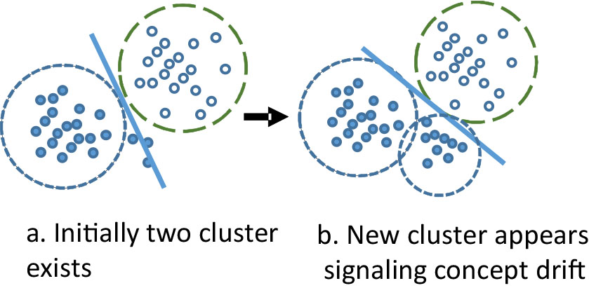

The limitation of clustering based approach is that if global data distribution does not create new dense regions, then the detection will fail. This is explained in detail using algorithm by Kantardzic et al [12]. The algorithm assumes that samples of the same class form clusters. The detection process is illustrated by Fig. 5. In Fig. 5a, two existing clusters of samples are divided by a linear classification model. Some newly arrived samples fall out of the existing clusters, but the density of the new samples is low. The learning model does not need adjustment. After some time more samples arrived outside of the original clusters. These new samples form a dense third cluster as shown in Fig. 5b. This event signals the framework that a potential drift has occurred. A new learning model is trained in response. This approach is best used for non-stationary drift. New clusters cannot be detected if drift occurs within the original clusters. Only when new data appear in new area can this approach detect change. The case for detection failure is demonstrated in Fig. 6. In Fig. 6b, all new samples fall within the existing cluster, which does not trigger drift detection. Without labels, it is also impossible to differentiate differences of the new samples from current samples within the cluster. Therefore, this approach cannot detect drift under this scenario.

Figure 6.

Clustering based concept drift fail to detect when drift is stationary.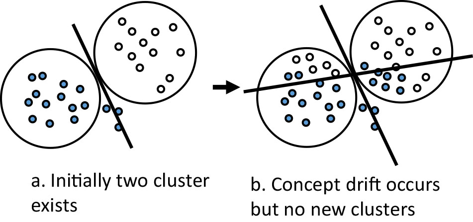

Tu and Chen [31] proposed a framework that has an online component that map each data samples to a grid in the data space, and an offline component that compute grid density. A density decaying mechanism was applied to forget older samples so that new dense grid can be discovered. An ensemble-based grid density framework was proposed by Sethi et al. [24] to tackle concept drift in both spatial and temporal component of the data stream A grid of the data space is generated by dividing each feature of the data into fixed intervals, forming a grid. As samples arrive, they are assigned to their specific grid cell based on their feature values. The number of samples in each cell is recorded, and the cell becomes dense if the number rises beyond a threshold $p$ . If at a moment a normal cell becomes dense, then it is clear that more data are arriving in the data space occupied by the cell, a potential concept drift. The grid detection has similar limitations to the clustering based approach. The Grid Based Detection monitors changes in the shape of the data. If all new data only arrive in existing dense grids, then the overall shape of the data will not change. Since the data is unlabeled, it is impossible to track the shape of individual class of data. This limitation is shown in Fig. 7. Figure 7a shows the initial decision boundary between the two classes with three dense grid. Figure 7b, new samples arrives mostly in existing dense grids, but clearly decision boundary is shifted. This scenario cannot be detected by Grid Based drift detection. For this reason, in an unsupervised environment, this algorithm is best when used for non-stationary drift

Figure 7.

Grid based drift detection failed to detect drift.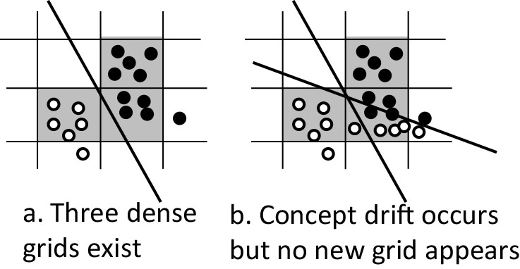

3.3 Learning model based approaches

This group of detection algorithms use the underlying classification model’s characteristics for concept drift detection. Dries et al. [6] proposed three approach in their study: a) density estimation on binary representation of the data, b) measures average margin of 1-norm SVM and c) average error rate generated by SVM. The study shows that the SVM approach (second approach) has the best precision and recall. The linear SVM creates a margin between two supports. Concept drift can be detected if there are significant changes between the margins. Sethi et al. [25] further improve the margin approach by extending it to partially labeled data stream. The approach (MD3) computes the density within a margin created by decision boundary and support of a linear SVM trained on original training data. Once the SVM is trained, the detection process does not require labels. The margin density is calculated by Eq. (1).

$\displaystyle\rho=\frac{\#\text{samples with abs}\left(w\cdot x_{i}+b\right)% \leqslant 1}{\text{\#samples}}$ (1)

#samples is the number of data samples within the current time step in data stream. The separating hyperplane of the SVM is defined by $w\cdot x+b=$ 0. The function abs() calculate the absolute value. For each sample $i$ , if $abs(w\cdot x_{i}+b)\leqslant 1$ , then it falls between the defined margin. The maximum and minimum $\rho$ are monitored for the current chunk. If $\rho$ falls outside of the existing min-max range, then a potential drift is detected. The process is illustrated in Fig. 8. Initially in Fig. 8a, two classes of samples are separated by a horizontal decision boundary, with margin density 0.4 (2 out of 5 samples inside margin) and 0.5 (3 out of 6 samples inside margin) for each class respectively. After concept drift occurs in Fig. 8b, the decision boundary changed, as a result the margin density changes to 0.8 (4 out of 5 samples inside margin) and 0.66 (4 out of 6 samples inside margin) respectively. After retrain SVM, the new decision boundary reflects post-drift reality in Fig. 5c, and the margin density returns to normal value of 0.6 and 0.5 respectively.

Figure 8.

Illustration of margin density drift detection.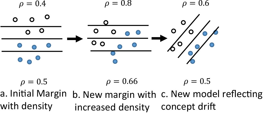

Figure 9.

Margin density failed to detect concept drift.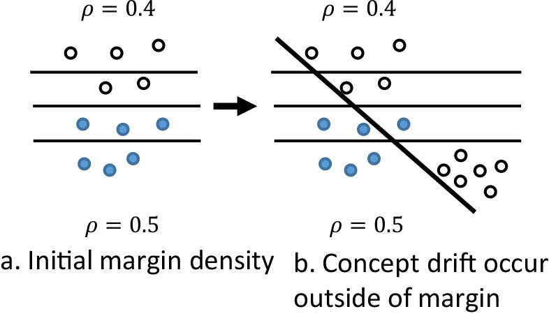

Figure 10.

HEFDD ensemble structure.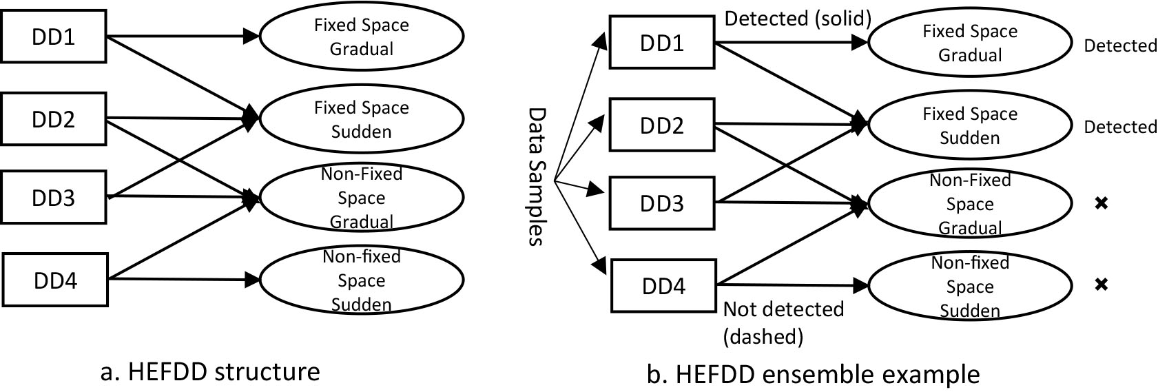

This approach is best used for stationary drift since the density is only calculated within a narrow region encompassing the decision boundary. The margin density will not change if data suddenly appear in a new region outside of the margin. Thus, the margin density approach will fail. This is demonstrated in Fig. 5. A new area of samples suddenly appear outside of the initial margin shown in Fig. 9a. Since this new group of samples does not impact the density within the margin, it would not be detected by Margin Density Drift Detection. However, clearly the old decision boundary (dash line in Fig. 9b should be replaced by the new boundary (solid line in Fig. 9b).

4. Heuristic ensemble framework for drift detection

Many distribution based concept drift detection algorithms has limitations on which type of concept drift they are able to detect when labeled data aren’t available. The limitations is the result of their assumption about specific nature of the concept drift. For instance, Clustering and Grid approaches assume that concept drift occur when new dense regions in the data space appear. But there are many cases where drift can occur in existing data regions. On the other hand, Margin Density approaches assume concept drift will be captured around existing data models, but there can be changes happening far away. Kolmogorov-Smirnov (KS) Test can detect samples from different populations, but cannot identify changes from the same global population. The proposed framework, Heuristic Ensemble Framework for Drift Detection (HEFDD) aims to detect all types of concept drift in data streams by combining the strength of multiple concept drift detection algorithms. HEFDD divide data stream into chunks, where each chunk is a fixed number of data stream samples [25]. This strategy is used because it is most flexible, as it can work with both chunk based detection algorithm and incremental detection algorithm [5].

4.1 Ensemble and heuristic voting

The ensemble of HEFDD is consists of individual concept drift detection algorithms, illustrated in Fig. 10a, which shows one example of possible configurations of the drift detection ensemble. Each DD (DD1 to DD4) stands for a single Drift Detection algorithm. The arrows in Fig. 10a denote which concept drift type each DD is able to detect (DD1 is able to detect Fixed Space Gradual and Fixed Space Sudden, DD2 is able to detect Fixed Space Sudden and Non-fixed Space Sudden and so on). This is determined by analyzing theoretical approach used in a specific technique and on the experimental results of each concept drift detection algorithm. DD1 may have similar assumption on concept drift to Margin Density, and therefore it can only detect Fixed Space drifts. On the other hand, DD4 may have similar assumption to Clustering, so only Non-fixed Space drift can be detected. Each algorithm votes on the type of concept drift it can detect. Votes are not counted globally. Instead each type of concept drift keeps track of votes from the subset of techniques that can detect it. In Fig. 10a, Fixed space Sudden and Non-fixed Space Gradual both potentially have three techniques’ vote while Fixed Space Gradual and Non-Fixed Space Sudden both potentially have one technique’s vote. As long as a concept drift type obtains a majority voting on its own total vote count, it is detected by HEFDD. This is further illustrated in Fig. 10b. As a chunk of data samples arrives, they are directed through each of the DDs. Solid arrows following the DD1 and DD2 means a concept drift is detected in the current chunk whereas dashed arrows following DD3 and DD4 means a concept drift is not detected. Based on heuristic voting, Fixed Space Gradual (FSG) is detected because it received one vote out of one total vote. Fixed space Sudden (FSS) is also detected because it received two votes out of three total vote, reaching a majority. Non-fixed space Gradual (NFSG) is not detected because it only received one vote out of three, and finally Non-fixed Space Sudden (NFSS) is also not detected by not receiving any vote. The pseudocode for the algorithm is summarized in Algorithm 1.

Table 2
Different concept drift detection algorithms detect different types of drift

Algorithm	FSS	FSG	FSI	NFSS	NFSG	NFSI
Margin Density [25]	YES	YES	YES	NO	NO	YES
Clustering [12]	NO	NO	NO	YES	YES	YES
KS Test [28]	NO	NO	NO	YES	YES	YES
Grid [24]	NO	NO	NO	YES	YES	YES

Algorithm 1: Algorithm for HEFDD Ensemble
Input: Data Chunk C, Array of Detection Algorithm A
Output: Array of Concept Drift Types Detected
Initialization:
D $=$ Array of integers, each corresponds to how many times one drift type is detected.
C $=$ Array of True and False, each corresponds to whether one type of drift is detected
1: for each a in A:
2: detect concept drift in C using a
3: if detected:
4: Increment corresponding integer in D
5: for each d in D:
6: if $d>$ Length(A)/2
7: Set corresponding True/False in C
8: return C

Figure 11.

Synthetic data with fixed-space and non-fixed space drift.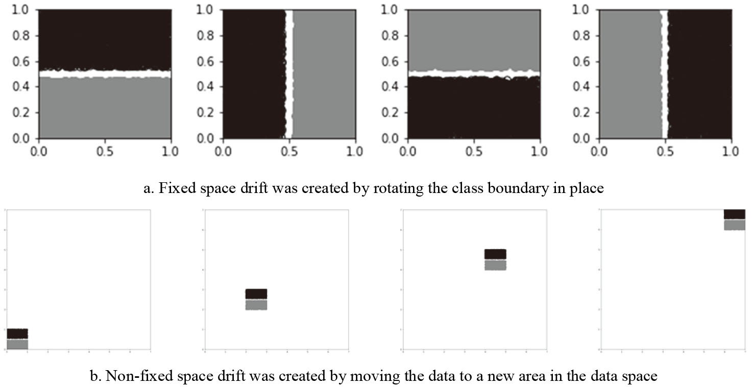

4.2 Component selection for HEFDD

The selection of algorithm that constitute the ensemble is based on two principles:

a)
type of concept drift to be detected
b)
heuristic analysis of each algorithm

In this study six types of concept drift are identified by combining the speed and distribution classifying criteria, outlined in Section 2. Ideally, there should be several detection algorithms in the ensemble that is able to detect each of the six concept drift types. To increase confidence of detection and reduce false positive, each concept drift type is better to have more than one algorithm’s vote. In our review of algorithms in Section 3, we identified the limitations of Margin Density, Clustering, KS Test and Grid concept drift detection algorithms, which are summarized in Table 2. Margin Density can detected all Fixed Space concept drift while Clustering, KS Test and Grid can detect only Non-fixed Space drifts. An ensemble of these algorithms is therefore able to detect all six types of concept drift. At the same time, Non-fixed space type drifts will have three algorithm voting for improved detection through the voting process. If two algorithms reach a majority vote, then there is a higher confidence that such type of concept drift is truly happening.
5. Experiments

Experiments were conducted using both synthetic and real-world dataset. Synthetic datasets were created so that each of the proposed type of concept drift can be accurately simulated. These datasets were used to confirm our analysis of each individual algorithms in Table 2 and prove the concepts of HEFDD approach. Real-world datasets were used to show the advantage of HEFDD methodology when compared to a detection strategy using only a single drift detection algorithm.

5.1 Datasets

Synthetic dataset were 2-dimensional input with the third dimension a binary class label. Fixed space and Non-fixed space drifts were created as illustrated in Fig. 11. Fixed space data were created with normalized input in range [0, 1]. A margin width of 0.1 was defined between the two classes of samples. The margin rotates in place as more streaming samples were generated. Non-fixed space data were created by moving the data generation range from [0, 1] toward [6, 7]. In both fixed and non-fixed drifts, the rate of change is also modified to create abrupt, gradual and incremental drift. In abrupt drifts, all margin rotation and data movement are completed in one chunk of data, while in gradual and incremental drift they take three chunks to complete. In total, 6 separate synthetic data sets were created, covering all six concept types in Table 2. Each dataset has 20 chunks, where each chunk have 500 data samples. The speed of changes is generated by controlling how fast concept drift occurs. In the sudden drift datasets (FSS and NFSS), three separate concept drifts occur in chunk 5, 10 and 15. In the gradual and incremental drift datasets, three separate concept drifts occur from chunk 4 to chunk 6, from chunk 9 to chunk 11 and from chunk 14 to chunk 16.

Three real-world datasets were used in the experiments. Electric Market (EM) [21] dataset is a real-world dataset that keeps track of the rise and fall of electricity price [34]. Forest cover (Covtype) dataset contains forest cover type data from US Forest service [2]. Covtype was modified into a binary class dataset by selecting two classes with the most samples. SPAM dataset is a text dataset from SpamAssasin data collection (Blake and Merz, 1998). It contains a numerical representation of 6213 emails where some of these are spam emails. Although all available datasets contain class labels, the drift detection process does not take them into consideration to simulate unlabeled streaming data. Table 3 summarize the characteristic of each dataset and the size of data chunk used in the experiments.

Table 3
Dataset used in experiments

Name	# Samples	# Input attribute	# Classes	Chunk size
Synthetic (FSS, FSG, FSI, NFSS, NFSG, NFSI)	10,000	2	2	500
EM	45312	7	2	1500
Covtype	218515	54	8	2000
SPAM	6213	500	2	500

Table 4

Different concept drift detection algorithms detect different types of drift in synthetic data sets

[height=0.8cm,width=2.4cm]AlgorithmData sets	FSS	FSG	FSI	NFSS	NFSG	NFSI
Actual Drifts	5, 10, 15	4–6, 9–11, 14–16	4–6, 9–11, 14–16	5, 10, 15	4–6, 9–11, 14–16	4–6, 9–11, 14–16
Margin Density [25]	5, 10, 15	4, 5, 10, 15	4, 6, 9, 10,11, 14, 16	–	–	–
Clustering [12]	–	–	–	5, 10, 15	4, 9, 14	4, 5, 6, 9, 10, 15, 16
KS Test [28]	–	–	–	5, 10, 15	4, 9, 14	4, 6, 10, 11, 14, 15
Grid [24]	–	–	–	5, 10, 15	4, 9, 14	4, 5, 6, 9, 10, 11, 14, 15
HEFDD	5, 10, 15	4, 5, 10, 15	4, 6, 9, 11, 14, 16	5, 10, 15	4, 9, 14	4, 5, 6, 9, 10, 15

Table 5

Experimental result on real-world datasets

[dir=NW]AlgorithmData sets	Electric market			Spam
	Detection	Correct %	False positives	Detection	Correct %	False positives
DDM [7]	4, 7, 10, 13, 24	100%	0	4, 10	100%	0
Margin	5	20%	0	1, 4, 12	50%	2
Clustering	1, 7, 10	40%	2	2, 6, 7, 10	50%	2
KS Test	2, 7, 10	40%	2	4, 7	50%	1
Grid	7, 8, 9, 10	40%	1	7, 9, 10	50%	2
HEFDD	5, 7, 10	60%	0	1, 4, 7, 10, 12	100%	3
[dir=NW]AlgorithmData sets	Covtype			KDD’99
	Detection	Correct %	False positive	Detection	Correct %	False positives
DDM [7]	5, 9, 13, 16, 20, 23, 32, 34, 40, 42, 47	100%	0	7, 9, 10, 15, 17, 23, 36, 48	100%	0
Margin	4, 5, 8, 10, 18, 24, 42	36.3%	4	7, 8, 13, 20, 21,35	37.5%	3
Clustering	14, 17, 29, 33, 36, 38, 39, 40, 44, 46	54.5%	5	7, 15, 23, 25, 26, 32, 33, 34, 36, 37, 42	50%	6
KS Test	5, 7, 10, 18, 22, 23, 27, 33, 39, 47	54.5%	6	7, 8, 9, 12, 14, 21, 48, 49	50%	2
Grid	12, 13, 14, 20, 22, 26, 30, 33, 39, 40, 43	63.6%	8	3, 10, 13, 15, 20, 22, 23, 36, 40	50%	4
HEFDD	4, 5, 8, 10, 14, 18, 33, 39, 40, 42	63.6%	6	7, 8, 13, 15, 20, 21, 35, 36	62.5%	3

5.2 Experimental results

Table 4 shows the experimental results of four concept drift detection algorithm and their EFDD ensemble using synthetic data. For the fixed-space datasets, only Margin Density algorithm is able to detect any concept drift, which is expected result based on analysis in Section 3. Since Margin Density constitute the only vote for fixed-space drift, EFDD produces the same detection of this drift type as Margin Density. Among the three drift speeds, Margin Density is able to detect all cases of sudden drift. It has some detection delay and redundant detection for the FSG and FSI dataset. In the non-fixed space dataset, Clustering, KS Test, and Grid are able to detect any drift, also as expected. All algorithms detect NFSS and NFSG drifts without delay or redundancy. However, in NFSI, both algorithm created many redundant detection. EFDD is able to reduce the number of redundant detection requiring that at least two algorithm reaching a majority.

The exact location of concept drifts for synthetic data is determined in advance, but this is not the case for real-world dataset. To overcome this problem, a performance based algorithm DDM [7] is chosen as the golden standard since DDM is able to detect all types of concept drift using labeled samples. Table 5 shows concept drift detection for real-world data stream comparing with DDM’s detection result using labeled data, considered to be gold standard for the other five unlabeled drift detection methodologies. The detection column shows the chunk number where drift is detected and the accuracy column shows the corrected detection compared to DDM. Looking at the exact chunk number, HEFDD only correctly detected two chunks out of five from DDM. However, different algorithms have different sensitivity for concept drift. In addition, gradual and incremental drift may have a delayed detection because the change is very slow. For this reason, it is more useful to also consider adjacent chunks detection as hit when comparing drift detection result. That is, if chunk detection is only off by one chunk when compared to golden standard approach DDM, it is still considered the same detection. To better show detections that are adjacent, a notation A(B) is adopted where A is chunk number detected by any algorithm other than DDM and B is chunk number detect by golden standard DDM. The accuracy column is calculated by dividing the number of correctly detected concept drift from each algorithm with the total number of detection by the gold standard approach. Since different algorithms have different sensitivity towards change detection, the data chunk that is adjacent to correct detection are also counted. For instance, Margin detected chunk 5 with concept drift in the Electric Market while DDM detected chunk 4. Since chunk 5 is adjacent to chunk 4, due to algorithm sensitivity this is counted as a correct detection.

Figure 12.

Concept drift detection accuracy and number of false positive detection compared across algorithm in real-world dataset experiments.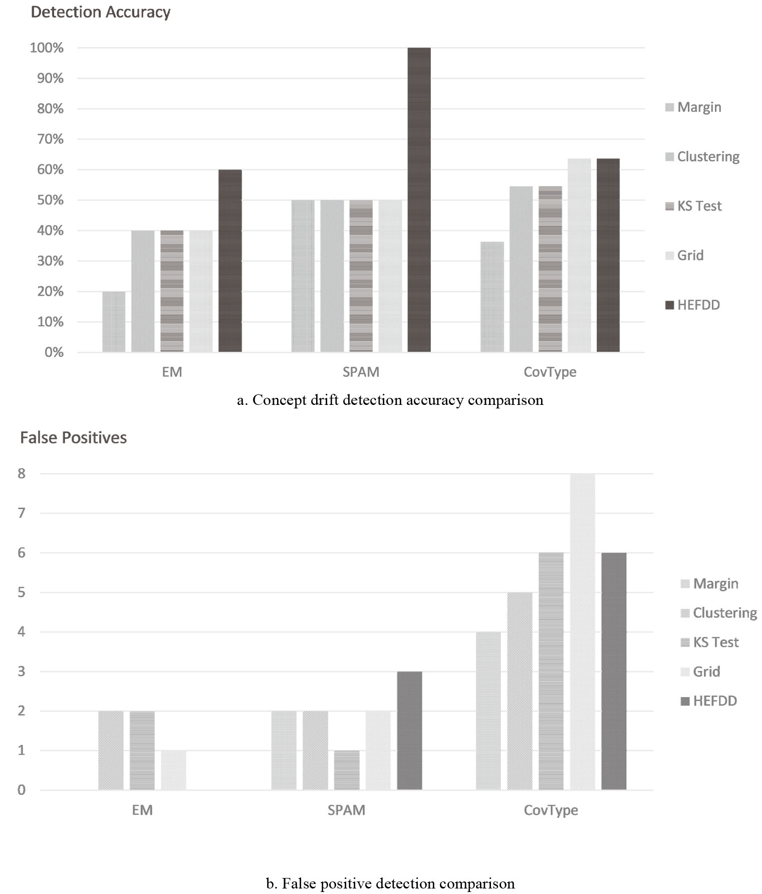

5.3 Discussion

The synthetic dataset shows that the heuristic analysis of each algorithm match their respective concept drift detection types. Margin density is able to detect all Fixed Space types but fails on all Non-fixed space types. Clustering, KS Test and Grid are able to detect all Non-fixed space types but fail on Fixed Space types. The speed of drift impacts the accuracy and precision of each detection algorithms. Ideally, concept drift detection algorithm should be able to detect a concept drift as early as possible and at the same time maintain a high precision and accuracy of detection. For example, in FSI ideal detection should detect concept drift at the beginning of chunk 4, 9 and 14. Margin density has chunk 6, 11, and 16 as redundant drift detection since they are the same drift started in chunk 4, 9 and 14. In real-world applications, because concept drifts are detected in these chunks, a streaming classification framework will likely spend resources on training new models. HEFDD helps by reducing the redundant detection in NFSI so that less resources are wasted.

The Electric Market column of Table 5 shows detection results for the EM dataset. After taking into account of drift sensitivity, EFDD is able to detect three drifts compared to DDM at chunk 5(4), 7(7) and 10(10). HEFDD detections at chunk 7(7) and 10(10) came from detection majority by Clustering, KS Test and Grid while chunk 5(4) is contributed by Margin. The EM stream dataset shows mostly non-stationary drift in the beginning, while stationary drift starts to appear at the middle of the stream. This confirms our hypothesis that real-world datasets may contain more than one type of concept drifts. Together, HEFDD is able to detect 60% of DDM’s detections, more than any individual algorithms that made up the

HEFDD ensemble. The Spam column in Table 5 shows Margin density correctly detected 4(4) with 12(10) as near miss being two chunks away from chunk 10. Clustering, KS Test and Grid produced majority at chunk 7 and a correct detection at chunk 10(10). Together, EFDD detected 100% DDM’s detection at 4(4) and 10(10), but with false positive at chunk 1, 7 and 12. The Covtype colum in Table 5 shows Margin density correctly detected 4(5), 5(5), 8(9), 10(9), 24(23) and 42(42). Since chunk 4, 5 correspond to DDM detection of chunk 5 and chunk 8, 10 correspond to DDM’s chunk 9, these four detections by margin density really are detecting only two drifts. EFDD is able to detect more drift than Margin Density and Clustering, and detect the same number of drift with Grid. Counting false positive, EFDD has the lowest number of false positives compared to the other three algorithms. Averaging three dataset’s detection accuracy, statistical p-value test using $z$ -score shows HEFDD has significance improvement at $p<$ 0.05.

Figure 12 summaries and compares the result of all four experiments. Fig. 12a plots the accuracy of correctly detected concept drift as listed in Table 5. It is clear that in most cases EFDD is able to detect more drifts than any individual algorithm. Exceptions are in hyperplane where EFDD detected the same number as Margin Density and in Covtype where EFDD equals Grid. Figure 12b shows the percentage of false positive detected by all four algorithms. The percentage is produced by dividing number of false positive detection by number of drift detected by DDM. For instance, for hyperplane, there is one false positive by Margin Density and four drift detected by DDM. The false positive percentage is therefore 25%. The result shows the ability of EFDD to reduce the number of false positives compared to individual algorithms. In hyperplane, EFDD has more false positive than Cluster, KS Test and Grid because the latter three algorithms could not detect any drift. For real-world data sets, EFDD is able to reduce false positive in EM and Covtype dataset. To reduce false positives, a more diverse set of detection algorithms might be needed [11]

6. Conclusion

Streaming data classification requires adaptive data mining framework which is able to detect concept drifts and adapt classification model to these changes. The complexity of real-world application requires an approach to cope with different types of concept drift to be detected in streams without labeling samples. Existing detection algorithms, which focus on only one type of concept drift, might not be able to detect drift in real-world streaming data where multiple types of concept drift occur. An ensemble framework, called Heuristic Ensemble Framework for Drift Detection (HEFDD), is proposed, implemented and evaluated in this paper. HEFDD employs an ensemble of state-of-the-art concept drift detection algorithms with heuristic voting mechanism. Concept drift is detected as long as majority voting is reached for a specific type of concept drift. After each type of concept drifts is voted, the union of detection decisions for all types of drift is produced as the final detection decision. HEFDD was implemented using Margin Density, Clustering, Kolmogorov-Smirnov (KS) Test and Grid-Based drift detection algorithms as components of the ensemble. Stationary drifts are covered by Margin Density approach while non-stationary drifts are covered by Clustering, KS test and Grid-Based approach.

HEFDD was tested with synthetic and real-word dataset, including EM, Covtype and SPAM. For synthetic data set experiments, it is verified that different algorithms detect different types of drift, confirming our heuristic analysis. In real world experiment, HEFDD shows significant improvement at $p<$ 0.05 using $z$ -score test when compared to individual drift detection algorithm. In EM and Covtype HEFDD outperforms Margin Density by as much as 10% accuracy because it is able to detect more concept drifts in the stream.

Future study should include more concept drift detection algorithms in the ensemble to increase detection accuracy and reduce false alarms. Also, it is possible to utilize the information provided by HEFDD’s detections and design an improved semi-supervised or unsupervised streaming data classification framework. HEFDD enables such framework to react to different types of concept drift differently, which has the potential to optimize the way new classification models will be trained after drift is detected.

References

Ahmadi

Beigy

. Semi-supervised ensemble learning of data streams in the presence of concept drift. InInternational Conference on Hybrid Artificial Intelligence Systems. Springer, Berlin, Heidelberg, 2012 Mar 28, pp. 526-537.

Blackard

Dean

. Comparative accuracies of artificial neural networks and discriminant analysis in predicting forest cover types from cartographic variables. Computers and electronics in agriculture. 1999 Dec 1; 24(3): 131-51.

Borchani

Larranaga

Gama

Bielza

. Mining multi-dimensional concept-drifting data streams using Bayesian network classifiers. Intelligent Data Analysis. 2016 Jan 1; 20(2): 257-80.

Cabanes

Bennani

. Change detection in data streams through unsupervised learning. In The 2012 International Joint Conference on Neural Networks (IJCNN), IEEE, 2012 Jun 10, pp. 1-6.

dos Reis

Flach

Matwin

Batista

. Fast unsupervised online drift detection using incremental kolmogorov-smirnov test. InProceedings of the 22nd ACM SIGKDD International Conference on Knowledge Discovery and Data Mining, 2016 Aug 13, pp. 1545-1554.

Dries

Rückert

. Adaptive concept drift detection. Statistical Analysis and Data Mining: The ASA Data Science Journal. 2009; Dec; 2(5-6): 311-27.

Gama

Medas

Castillo

Rodrigues

. Learning with drift detection. In Brazilian symposium on artificial intelligence, Springer, Berlin, Heidelberg, 2004 Sep 29, pp. 286-295.

Gama

Žliobaitė

Bifet

Pechenizkiy

Bouchachia

. A survey on concept drift adaptation. ACM computing surveys (CSUR). 2014 Mar 1; 46(4): 1-37.

Glazer

Lindenbaum

Markovitch

. Learning high-density regions for a generalized kolmogorov-smirnov test in high-dimensional data. Advances in Neural Information Processing Systems. 2012; 25: 728-36.

10.

Kantardzic

Lyu

. Detecting different types of concept drifts with ensemble framework. In 2018 17th IEEE International Conference on Machine Learning and Applications (ICMLA), IEEE, 2018 Dec 17, pp. 344-350.

11.

Johnson

Giraud-Carrier

. Diversity, accuracy and efficiency in ensemble learning: An unexpected result. Intelligent Data Analysis. 2019 Jan 1; 23(2): 297-311.

12.

Kantardzic

Ryu

Walgampaya

. Building a new classifier in an ensemble using streaming unlabeled data. InInternational Conference on Industrial, Engineering and Other Applications of Applied Intelligent Systems, Springer, Berlin, Heidelberg, 2010 Jun 1, pp. 77-86.

13.

Khamassi

Sayed-Mouchaweh

Hammami

Ghédira

. Self-adaptive windowing approach for handling complex concept drift. Cognitive Computation. 2015 Dec; 7(6): 772-90.

14.

Khamassi

Sayed-Mouchaweh

Hammami

Ghédira

. A new combination of diversity techniques in ensemble classifiers for handling complex concept drift. In Learning from data streams in evolving environments, Springer, Cham, 2019, pp. 39-61.

15.

Kifer

Ben-David

Gehrke

. Detecting change in data streams. In VLDB 2004 Aug 31; 4: 180-191.

16.

Lazarescu

Venkatesh

Bui

. Using multiple windows to track concept drift. Intelligent Data Analysis. 2004 Jan 1; 8(1): 29-59.

17.

Lee

Magoules

. Detection of concept drift for learning from stream data. In 2012 IEEE 14th International Conference on High Performance Computing and Communication & 2012 IEEE 9th International Conference on Embedded Software and Systems, 2012 Jun 25. IEEE, pp. 241-245.

18.

Masud

Chen

Khan

Aggarwal

Gao

Han

Thuraisingham

. Addressing concept-evolution in concept-drifting data streams. In 2010 IEEE International Conference on Data Mining, 2010 Dec 13. IEEE, pp. 929-934.

19.

Minku

Yao

. DDD: A new ensemble approach for dealing with concept drift. IEEE Transactions on Knowledge and Data Engineering. 2011; Feb 24; 24(4): 619-33.

20.

Minku

White

Yao

. The impact of diversity on online ensemble learning in the presence of concept drift. IEEE Transactions on Knowledge and Data Engineering. 2009 Jul 6; 22(5): 730-42.

21.

Newman

. UCI repository of machine learning databases, University of California, Irvine. http://www.ics.uci.edu/mlearn/MLRepository.html. 1998.

22.

Pinage

dos Santos

da Gama

. Classification systems in dynamic environments: an overview. Wiley Interdisciplinary Reviews: Data Mining and Knowledge Discovery. 2016 Sep; 6(5): 156-66.

23.

Ross

Adams

Tasoulis

Hand

. Exponentially weighted moving average charts for detecting concept drift. Pattern Recognition Letters. 2012 Jan 15; 33(2): 191-8.

24.

Sethi

Kantardzic

. A grid density based framework for classifying streaming data in the presence of concept drift. Journal of Intelligent Information Systems. 2016 Feb 1; 46(1): 179-211.

25.

Sethi

Kantardzic

. On the reliable detection of concept drift from streaming unlabeled data. Expert Systems with Applications. 2017 Oct 1; 82: 77-99.

26.

Sethi

Kantardzic

Lyu

Chen

. A dynamic-adversarial mining approach to the security of machine learning. Wiley Interdisciplinary Reviews: Data Mining and Knowledge Discovery. 2018 May; 8(3): e1245.

27.

Siahroudi

Moodi

Beigy

. Detection of evolving concepts in non-stationary data streams: A multiple kernel learning approach. Expert Systems with Applications. 2018 Jan 1; 91: 187-97.

28.

Sobolewski

Wozniak

. Concept drift detection and model selection with simulated recurrence and ensembles of statistical detectors. J Univers Comput Sci. 2013 Feb 28; 19(4): 462-83.

29.

Song

Jermaine

Ranka

. Statistical change detection for multi-dimensional data. InProceedings of the 13th ACM SIGKDD international conference on Knowledge discovery and data mining, 2007 Aug 12, pp. 667-676.

30.

Spinosa

de Leon

. de Carvalho

Gama

. Olindda: A cluster-based approach for detecting novelty and concept drift in data streams. In Proceedings of the 2007 ACM symposium on Applied computing, 2007 Mar 11, pp. 448-452.

31.

Chen

. Stream data clustering based on grid density and attraction. ACM Transactions on Knowledge Discovery from Data (TKDD). 2009 Jul 28; 3(3): 1-27.

32.

Verdecia-Cabrera

Blanco

Carvalho

. An online adaptive classifier ensemble for mining non-stationary data streams. Intelligent Data Analysis. 2018 Jan 1; 22(4): 787-806.

33.

Webb

Hyde

Cao

Nguyen

Petitjean

. Characterizing concept drift. Data Mining and Knowledge Discovery. 2016 Jul; 30(4): 964-94.

34.

Zliobaite

Bifet

Pfahringer

Holmes

. Active learning with drifting streaming data. IEEE Transactions on Neural Networks and Learning Systems. 2013 Jan 17; 25(1): 27-39.

Heuristic ensemble for unsupervised detection of multiple types of concept drift in data stream classification

Abstract

Keywords

1. Introduction

2.2 Combinations of drift types by speed and distribution

3.1 Statistical test based approaches

3.2 Density based approaches

4.1 Ensemble and heuristic voting

Table 2 Different concept drift detection algorithms detect different types of drift

5.1 Datasets

Table 3 Dataset used in experiments

6. Conclusion

References

Table 2
Different concept drift detection algorithms detect different types of drift

Table 3
Dataset used in experiments