
Abstract
Dynamic social network analysis basically deals with the study of how the nodes and edges and associations among them within the network alter with time, thereby forming a special category of social network. Geometrical analysis has been done on various occasions, but there is a difference in the approximate distances of nodes. Snapshots for social networks are taken at each time slot and then are bound for these studies. The paper will discuss an efficient way of modeling dynamic social networks with the concept of neighborhood theory of cellular automata. So far, no model that uses the concept of neighborhood has been proposed to the best of our knowledge and the literature survey. Besides cellular automata that has been important tool in various applications has remained unexplored in the area of modelling. To this extent the paper, is the 1st attempt in modelling the social network that is evolving in nature. A link prediction algorithm based on some basic graph theory concepts has also been additionally proposed for the emergence of new nodes within the network. Theoretical and programming simulations have been explained in support to the model. Finally, the paper will discuss the model with a real-life scenario.
Introduction
A collection of associations among individuals is defined as a social network. The nature of how these individuals, commonly referred to as social entities, interact with one another is explained by social networking. Most of the social networks are dynamic. Individual associations in such networks tend to develop, persist for a period of time, and then degrade [1]. SNA (social network analysis) is a process for investigating social systems using networks and graph theory. Graph theory depicts a network structure as nodes, which might be individual actors, people, or things inside the network, and ties, edges, or links, which define linkages or interactions that connect them [2].
Despite the fact that several aspects of “social” and “group” dynamics have been learned in the sociological literature [3, 4], various mathematical techniques used in SNA have concentrated upon graph-theoretic features of social networks without giving attention to the dynamic behavior that exists among them. The majority of social network models have focused on special procedures such as random walks, contagion, and percolation [5, 6]. During the past few years, some important work has been done in bridging the gap between SNA and dynamical systems, thereby conceptualizing novel approaches to Dynamical Social Network Analysis (DSNA) [7] and temporal or evolutionary networks [8].
While modeling the method that the network follows for its alteration with time, a great impact is shown on the entire network, defining the innovative extent of the productivity in understandability of the procedures that motivate the development of these social networks. The computation of all the paths in a graph representing a social network is basically expensive, making it less efficient. One of the possible solutions is the usage of spectral methods for embedding a graph within a geometric space and carrying out further applicable calculations surrounded by geometry [9].
Researchers have been using Automata theory for the development of methods for providing the description and analysis of dynamic behavior for discrete systems. A special category of automata referred to as Cellular automata has been widely applied in various social science applications beyond their geographic feature basically since they can be successfully applied in simulation. Within the field of ecology, biology and the domain of medical science also Cellular Automata models have proven to useful and succeeding. The conception of space-time representation of Cellular automata has been explored in anthropology for modelling the development of societies, political science and sociology for exploration of civil violence, economics for representation of the procedures of urban agglomeration. Within each of the cases of discussed applications, humans are involved and the social interaction among humans has been somewhat that is considered to be explored. This motivation has initiated authors in the development of the model based on the cellular automata. Within the field of ecology, biology and the domain of medical science also Cellular Automata models have proven to useful and succeeding.
Cellular automata are characterized as a simplified model of a spatially extended decentralized system comprised of many unique parts known as cells, form a type of dynamic model with discrete time, space, and state properties. They are also defined as a type of finite-state machine where every cell within the model constitutes a finite quantity of states. A cellular automaton represents mathematical models that have simple guidelines that govern the duplications besides the destruction, which makes them applicable in modelling complex systems that constitute simple units. The existence of simple rules in cellular automata makes them applicable in the modelling of self-organizing networks that evolve with time. The feature of parallel computation, being local and conformism, adds to its effectiveness in modelling dynamic networks with understandability of global behavior with complex phenomena of several systems (networks) [10].
The objective of this paper is two-fold. This paper is an attempt to develop a dynamic social network model using the concept of neighborhood of cellular automata. While defining the evolution of new nodes within the network with this notion, the authors have proposed a novel link prediction approach, that will choose new nodes within the network that are only within the Von-Neumann neighborhood.
The paper is organized as follows. In Section 2, the authors have made a discussion of the various literature available in the field of study. Further considerations in modeling dynamic social networks and some required concepts are illustrated throughout Sections 3 and 4. Section 5 includes a full description of the dynamic social network model as well as a discussion of the suggested link prediction algorithm. Section 6 discusses the theoretical and simulation results generated in implementation of the proposed model. Finally, the paper presents with a real-time example related to the proposed model and ends with a general conclusion and future study in the area.
Literature review
Quite a few studies have been done in the area of modeling the structure and the dynamic behavior of social networks in the past decade. A few such works have been briefly illustrated in the present section. Kumar et al. [11] did research on Node-based approaches, concentrating on the expansion of the structure of online social networks (Flickr and Yahoo 360!) and explaining them with the dynamics of invitations. On the basis of the outcomes generated, a model was deduced that discusses its process as a composition of two steps. The addition of nodes, edges, and non-fading prevailing associations is considerable within this model. Furthermore, Leskovec et al. [12] have conducted an analysis at a local level with different platforms. Among various factors effecting the dynamics of networks, it was evaluated that edge locality has a significant impact on the development of networks. The technique of maximum likelihood was utilised for the comparison of models that render the probability of engendering the experiential data. A model illustrating the development of a network has been developed where the dissemination of new nodes within a graph has been stated through an exponential or polynomial function. Toivonen [13] in his thesis targets the increment of understandability concerning the way huge social networks are arranged besides the ways in which these networks are clarified, which includes the following: 1) A model based on simple local machinery that will illustrate genuine community structure has been devised to explain the requirements of social network models. 2) A well-defined comparative analysis for social network models that would judge their workability with real-world data would be conducted. 3) Various conflicting options were studied that would focus on the development of communities that have still been unexplored.
Considering frequent pattern-based methods, Bringmann et al. [14] has offered a substitute method defining certain rules for modeling structural alterations within a network. The proposed method shall be to represent the data-set through the collapse of every graph to a single undirected graph, accompanied by the addition of time-slots with every association upon their first appearance within the network. In order to illustrate how a network evolves, an attempt was also made to find association rules among the frequent patterns of interaction (sub-graphs). The researchers developed GERM (Graph Evolution Rule Miner) to extract evolution rules from graphs, and it was tested on four real-world networks (Flickr, Y360, DBLP, and arXiv) with varying time periods. The authors of [15] thought about how node centrality affected how structure changed over time. Experimentation has been done on large networks of email, through the sampling of sub-graphs for each of the data intervals for a day. Porter and Smith [16] proposed a technique for representing the structure of large social networks utilizing the concept of ego- centered network neighborhoods in their study. Such a study provided a localized picture of the network with a focus on the vertices and their kth order neighborhoods, enabling the finding of interesting patterns with network properties that are typically missed during global network analysis. The approach was verified with several real-life scenarios and was found to be successful in determining the network behavior on a local level. Some additional approaches were presented for the usage of these concepts in the identification of unexpected abnormalities within dynamic networks.
Within [17], authors have characterized the performance of a network through the scrutiny of associations among the promising prevailing triads. With the intention of discussing the development patterns within a network, the derivation of a probabilistic model was done for the calculation of probabilities for transitions between triads of nodes. The mean values of the transition triad matrix TTM, which presents a probability of a given pattern (
Some work on bio-inspired methods has been done by authors in [18]. They modeled the dynamics of the coauthor network using the forgetting curve and swarm intelligence. Professional relations were encouraged through social ant behavior. Investigations were conducted on a set of DBLP network authors’ assistances. In order to describe how email-based social networks develop, Budka et al. [19] employed a molecular-inspired socio-dynamical model as inspiration. Considerations were made regarding the formation and desertion of associations. Besides, alterations in relationship strength with time have also been studied. The research approach has been to study the social dynamics that prevail in various circumstances with some organizational tools that evolved from complexity theory [20]. Additionally, contemplating the fact of online social media serving as a platform for distinct expression in addition to public dialogue, it was estimated that the study, as multifaceted adaptive systems, will meaningfully subsidies understandability, prediction, and observation of social phenomena that occur in various online and offline social networks.
Structural changes within social networks have been discussed by Aouay et al. [21] with the classification of methodologies into three broad categories: methods that use node attributes information; ways for extracting various patterns inside a graph and modeling structural changes; and methods for simulating network growth over time using bio-inspired sources. Skillicorn et al. [9] investigated spectral techniques for modeling time-varying directed graphs. Snapshots for the network for every time period are destined to be joined together to form a single graph in such a way as to keep the structures associated with time. This global graph is thereafter said to be spectrally embedded. An observation is made on the similarity among certain set of nodes for tracking them over time, in such a manner that altering associations and clusters might be seen; with the conception that a meaningful trajectory is obtained for a node across time. There has been a demonstration of how these approaches are applied to comprehend how a social network changes as a result of internal dynamics and in response to cooperative law enforcement operations.
In the tutorial, the authors [8] intend to highlight concepts of control theory and the way it is applicable to social systems. It also engrossed classical prototypes of social dynamics and the way they are interrelated with the present achievements within multi-agent systems. The same authors have added a discussion of the most current comprehensive studies on MAS and complex networks. In addition to a study of the potential for control in social and techno-social systems, this paper places a strong emphasis on social processes that have arisen concurrently with MAS theory.
While modelling any dynamic social network, time has been an important constraint that has been explained in various ways by researchers around us. This time has been considered basically for the case of link prediction among the existing nodes within the network. Some focus is also made on whether the new nodes can come into picture. Considering the case of link production various temporal methods have been proposed. These temporal models are concerned with the fact that being provided with the link data from time 1 to
The authors [22] have combined a discussion on the diverse categories of cellular automata that have been used in modeling with a discussion on the various analytical methods for prediction of global behaviour from local configurations. A detailed sketch for the configuration of local settings under a global situation was also illustrated.
By using a parameter that represents the dimension of the hypercube that unites neighboring cells, the authors [23] established a general neighborhood for a d-dimensional cellular automaton that ranges from Von Neumann’s to Moore’s neighborhood. After the study of finite hypercube and hypertoruses, calculations are made on the quantity of neighbors within the boundary and connections within cells. The method makes use of ad-hoc software, which creates a Petri net sketch for the hypercube and hypertorus models.
Essential considerations in modeling dynamic social network
In the present section, the authors shall make a brief overview on the set of concepts that are required in the development of the proposed model. Initially, some useful concepts that will be useful in defining network dynamics will be defined:
Local density. The segment of first neighbors within state A (B, AB) for an agent is referred to as local density of A (B, AB) is represented by
Interface density. The degree of arrangement within systems is illustrated as the portion of links which join agents within diverse states. This segment is referred to as interface density. There is a decrement in this feature with the growth of homogenized domains in terms of size, which dissolves ultimately when either of the options triumphs. Within some consistent network topology, this factor provides an indication of average domain size, whereas within complex networks it illustrates rough domain growth like low interface density suggests a higher degree of organization. This factor is used in the study of the development of domains within individual understandings of stochastic dynamics, whereas average behavior for a system is illustrated as average interface density, and this average is considered for a collection of realizations commencing at dissimilar random preliminary circumstances [13].
Absorbing state. This state is reachable by interrelating agents whenever there is no further alteration of states by them, in addition to the dynamics halt. In some cases, agents that exist in a similar state are referred to as absorbing due to the nonexistence of neighbors within different states, such that the probability of node for alteration of states changes to zero.
Coarsening. This refers to the formation and development of reliable domains and is demonstrated with the lessening of interface density since it bears a resemblance to the growth of the extents of an average domain.
Meta-stable states. This state is referred to as a state within a dynamic system that exists for longer duration’s, although such a state has not been stretched by the system as an absorbing state. There are various types of meta-stable states, such as dynamical and trapped [13].
While explaining the link prediction algorithm, some of the basic features of the graph have been used. These features are illustrated as under:
Degree. For an undirected graph, the degree of any vertex ‘
Neighbors. A node
Common neighbor. Let ‘
Average degree of the network. If the Graph is considered to be an undirected one, then the average degree for the network is defined as summation of all the individual degrees of each node divided by the total number of nodes in the network. This criterion is often used in measuring the comparison between the number of edges and nodes a graph has.
Maximum path length: If the graph is a weighted connected graph and there exists ‘
Path with maximum traversed node: If there exist ‘
Preliminaries in DSN modeling
Defining dynamic social networks
Considering
With the considerations taken,
Objective function
In order to enumerate an eminence of any detected network communal arrangement, an extensively recognized portion referred as modularity
Usually,
Provided with a dynamic social network
Methods
A Dynamic Social Network replicates the alterations within a social network where the underlying network structure is frequently updated with the insertion and removal of nodes or edges. The introduction or removal of a certain group of nodes (or edges) over time can really be divided into a number of simultaneous insertions and deletions of nodes (or edges). This claim makes it easier to think of network changes as a collection of little operations, where each operation can be one of newNode, removeNode, newEdge, or removeEdge. These events are explained as under:
newNode: Familiarization of a new node u in-cooperation with its accompanying edges. u can come into existence with only a single edge connected to the existing network nodes. The choice of u should be within the von Neumann neighborhood of the existing nodes for the network.
removeNode: The removal of a node u and its subsequent associated edges from the network.
newEdge: Insertion of a new edge that connects two prevailing nodes comes into existence. The Link Prediction Algorithm, which is explained in the following section, will be used to select the node for link formation.
removeEdge: Removal of an existing edge e from the existing network [24].
The concept of neighborhood
With the consideration of the time dependent un-directed binary graphs
Considering
The graph
The darkened edges and vertices correspond to the elements in the network neighborhood anchored at vertex 6. The 3rd order neighborhood (i.e. 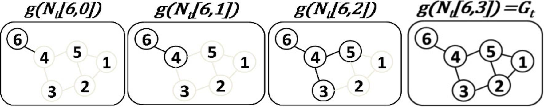
Neighborhood statistics
Considering an infinite integer lattice of dimension
Minkowsky distance:
Manhattan distance:
Minkowsky distance is generally represented as
Moore’s neighborhood for a cell
A square signifies specific cases of a 2-dimensional hypercube, concisely defined as a 2-cube. Though previously known for the 2-dimensional case, Von Neumann’s neighborhood is generalized into a d-dimensional instance that is clear-cut and employs a principle where the value changes for a single coordinate. In two dimensions, “two coordinates” also denotes “all coordinates”, which leads to uncertainty in Moore’s neighborhood’s generalization. In a
Surfaces of finite
Classical neighborhoods (2-dimensional case): a) von Neumann’s neighborhood; b) Moore’s neighborhood.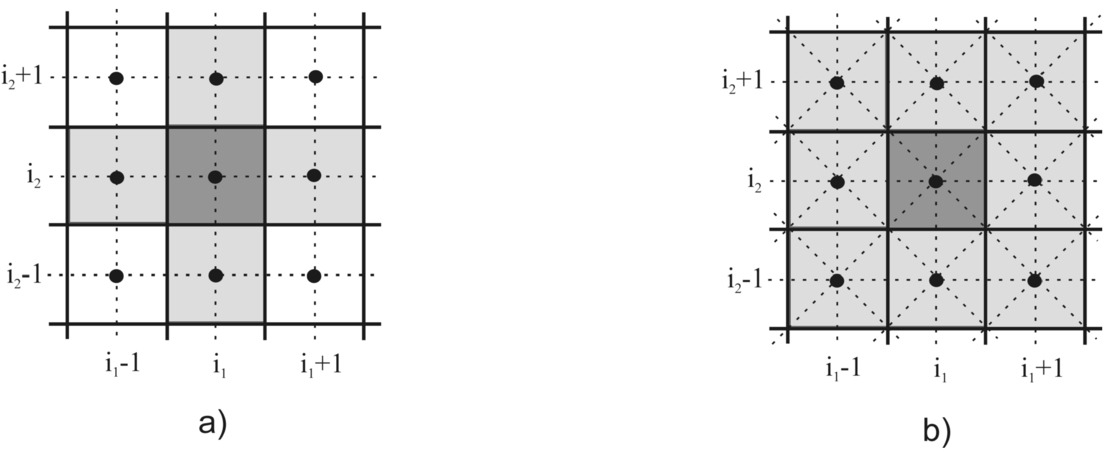
The proposed model of Dynamic Social Network has been illustrated in this section. Toward the maximum of our understanding as well as the review of literature, no framework that makes use of the notion of neighborhood has yet been provided. Other than cellular automata, which has been a crucial tool in many applications, modelling has not been fully investigated. This study represents the first attempt to simulate a social network that is naturally developing.
Figure 3 as illustrated below shall discuss the proposed model.
Model of the proposed system.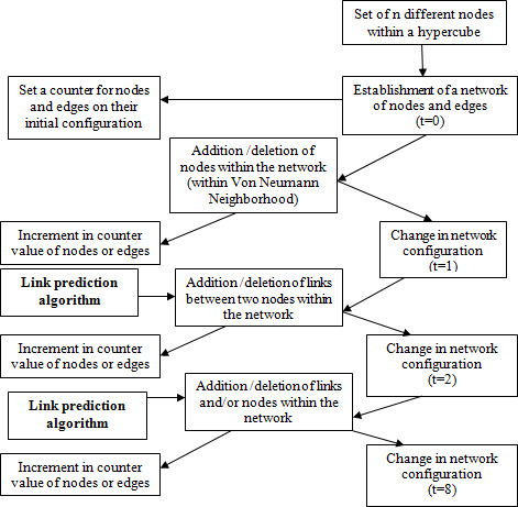
The above model can be distinctly separated into various phases:
Initialization phase Development phase Termination phase
During the initialization phase, the nodes and edges are defined. A set of nodes that reside within a particular dimension of a hypercube are taken into consideration for the setting of links within a network. At the same time, the number of nodes and edges are counted and the counter values for nodes and edges are set accordingly. The initial values for the counter are considered at time
During the development phase, there can be three possibilities. New nodes can come into existence within the hypercube, allowing development of links with the existing nodes and the development of new nodes and links at the same time. The three options can all show up simultaneously or separately. In each of these three cases, there is a change in the counter value. Time
[ht] Proposed Degree and von-Neumann neighborhood based Link prediction algorithm (DVNN-LPA)predictLinkFormationDeclare and Initialize
The next phase, i.e., the termination phase, appears after the continuation of the previous phase for a prolonged period. In this phase, there are no new nodes or edges developing for some time, and the counter value becomes constant for some time. This can be either because all the nodes have perished within the hypercube and there are no further chances of the new node appearing or because all the edges have been set up between the existing nodes and there are no further chances of the setting of a new edge with the application of the above algorithm. The proposed algorithm is better the the earlier algorithm in terms of consideration of the factors for link generation as this algorithm considers all the possible factors to be considered for link generation.
Within the present section, the authors shall be describing the proposed model and the Degree and Neighbor based algorithm. In the 1st part of the section a verification will be made taking into consideration of a random graph of 20 nodes. In the second part of the section, real life data sets will be considered and will be validated on the algorithm. Comparison results with earlier approaches have been drawn in the last part of this section.
Theoretical results
The random graph has been considered and checked on whether link formation is done on the set of nodes with the application of the above algorithm. A set of 20 nodes within a two-dimensional hypercube is considerably explained with graph paper (
Scenario 1: The 2nd criteria, as illustrated in the algorithm, i.e., the degree of the selected neighbor for link formation
Phase wise illustration of the formation of new Edges within Dynamic Social Networks according to Scenario 1.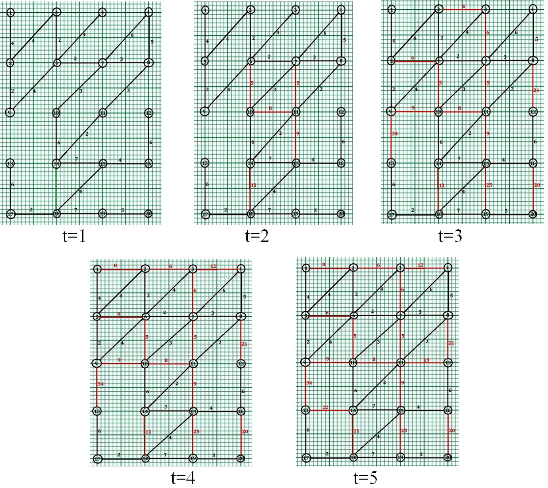
Phase 1 (
For node 7, there exist 4 neighbors namely 3, 6, 8, 11 and edge exist with 6 and 8, one with path length 2, other with path length 3. Only 11 is reachable from 8. Degree of 11 (2)
For node 10, there exist 4 neighbors namely 9, 6, 11, 14 and edge exist with 6 and 14, one with path length 5, other with path length 6. 9 and 11 is reachable from 6 and 14 respectively. Degree of 11 (3)
For node 11, there exist 4 neighbors namely 7, 10, 12, 15 and edge exist with 7 and 10, one with path length 5, other with path length 8. Node 15 is reachable only through two paths one through 10 and 14, other through 14. Degree of 15 (3)
For node 14, there exist 4 neighbors namely 10, 13, 15, 18, and edge exist with 10 and 15, one with path length 6, other with path length 7. 18 is reachable from 15. Degree of 18 (3)
For node 15, there exist 4 neighbors namely 11, 14, 19, 16, and edge exist with 11, 14 and 16, with path length 9, 7 and 4 respectively. Its neighbor 19 is not reachable 11, 14 or 16. Therefore, No node is selected for edge formation.
Phase 2 (
For node 3, there exist 3 neighbors namely 2, 7, 4, and edge exist with 2, with path length of 6. Degree of 7 (5)
For node 5, there exist 3 neighbors namely 1, 6, 9, and edge exist with 9 and 1, with path length of 2 and 4 respectively. Degree of 6 (5)
For node 8, there exist 3 neighbors namely 4, 7, 12 and edge exist with 4 and 7, with path length of 5 and 3 respectively. 12 is not reachable from 7 in any means. Therefore, No node is chosen for link formation.
For node 9, there exist 3 neighbors namely 5, 10, 13 and edge exist with 5, with path length of 2. Edge is possible with 10. Degree of 10 (4)
For node 12, there exist 3 neighbors namely 8, 11, 16 and edge exist with 16 with path length of 6. Edge possible with both 11 and 8. Degree of 11 (5)
For node 13, there exist 3 neighbors namely 9, 14, 17 and edge exist with 17 with path length of 6. Edge is possible with both 14 and 9. Degree of 14 (4)
For node 16, there exist 3 neighbors namely 12, 15, 20 and edge exist with 12 and 15 with path length of 6 and 4 respectively. Edge is possible with 20. Degree of 20 (1)
For node 18, there exist 3 neighbors namely 17, 14, 19 and edge exist with all with path length – 2, 11 and 7 respectively. Therefore, No neighbor node is left for link formation.
For node 19, there exist 3 neighbors namely 15, 18, 20 and edge exist with 18 and 20 with path length – 7 and 5 respectively. Edge is possible with 15. Degree of 15 (4)
Phase 3 (
For node 4, there exist 2 neighbors namely 3, 8 and edge exist with 8 path length 5. Edge is possible with 3. Degree of 3(3)
For node 17, there exist 2 neighbors namely 13, 18 and edge exist with both of them path length 6 and 2 respectively. Therefore, No neighbor bode is left for link formation.
For node 20, there exist 2 neighbors namely 16, 19 and edge exist with both of them path length 20 and 5 respectively. Therefore, No neighbor bode is left for link formation.
Phase 4 (
For node 7, there exist 4 neighbors namely 6, 3, 8, 11 and edge exist with all of them. Therefore, No neighbor bode is left for link formation.
For node 10, there exist 4 neighbors namely 6, 9, 11, 14 and edge exist with all of them. Therefore, No neighbor bode is left for link formation.
For node 11, there exist 4 neighbors namely 7, 10, 12, 15 and edge exist with 7, 10 and 15 with path length 5, 8 and 9 respectively. Edge possible with 12. Degree of 12 (2)
For node 14, there exist 4 neighbors namely 10, 13, 15, 18 and edge exist with 10, 15 and 18 with path length 6, 7 and 11 respectively. Edge possible with 13. Degree of 13 (2)
For node 15, there exist 4 neighbors namely 11, 14, 16, 19 and edge exist with all of them. Therefore, No neighbor bode is left for link formation.
Phase 5 (
For node 3, there exist 3 neighbors namely 2, 7, 4 and edge exist with all of them. Therefore, No neighbor bode is left for link formation.
For node 5, there exist 3 neighbors namely 1, 6, 9 and edge exist with all of them. Therefore, No neighbor bode is left for link formation.
For node 8, there exist 3 neighbors namely 4, 7, 12 and edge exist with all of them. Therefore, No neighbor bode is left for link formation.
For node 9, there exist 3 neighbors namely 5, 10, 13 and edge exist with all of them. Therefore, No neighbor bode is left for link formation.
For node 12, there exist 3 neighbors namely 8, 11, 16 and edge exist with all of them. Therefore, No neighbor bode is left for link formation.
For node 13, there exist 3 neighbors namely 9, 14, 17 and edge exist with all of them. Therefore, No neighbor bode is left for link formation.
For node 16, there exist 3 neighbors namely 12, 15, 20 and edge exist with all of them. Therefore, No neighbor bode is left for link formation.
For node 18, there exist 3 neighbors namely 17, 14, 19 and edge exist with all of them. Therefore, No neighbor bode is left for link formation.
For node 19, there exist 3 neighbors namely 15, 18, 20 and edge exist with all of them. Therefore, No neighbor bode is left for link formation.
Phase 6 (
For node 4, there exist 2 neighbors namely 3, 8 and edge exist with all of them. Therefore, No neighbor bode is left for link formation.
For node 17, there exist 2 neighbors 13, 18 and edge exist with all of them. Therefore, No neighbor bode is left for link formation.
For node 20, there exist 2 neighbors namely 16, 19 and edge exist with all of them. Therefore, No neighbor bode is left for link formation.
Since there is no more neighbor node left for link formation within the graph, the graph is complete.
Since there are no further development of the new edges within the graph after
Scenario 2: 2nd criteria as illustrated in the algorithm i.e indegree of the selected neighbor for link formation
Phase wise illustration of the formation of new Edges within Dynamic Social Networks according to Scenario 2.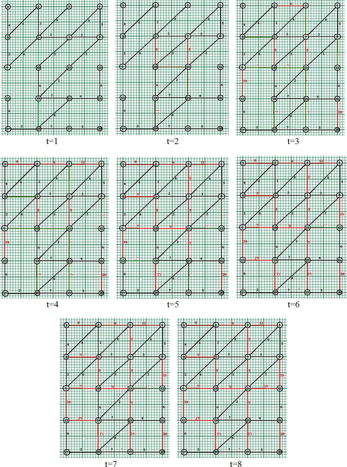
Phase 1 (
For node 7, there exists 4 neighbors namely 3, 6, 8, 11 and edge exist with 6 and 8, one with path length 2, other with path length 3. Only 11 is reachable from 8. Degree of 11 (2)
For node 10, there exists 4 neighbors namely 9, 6, 11, 14 and edge exist with 6 and 14, one with path length 5 and other with path length 6. 9 and 11 is reachable from 6 and 14 respectively. Degree of 11 (3)
For node 11, there exists 4 neighbors namely 7, 10, 12, 15 and edge exist with 7 and 10, one with path length 5, other with path length 8. 15 is reachable only through two paths one through 10 and 14, other through 14. Degree of 15 (3)
For node 14, there exists 4 neighbors namely 10, 13, 15, 18 and edge exist with 10 and 15, one with path length 6 and other with path length 7. 18 is reachable from 15. Degree of 18 (3)
For node 15, there exists 4 neighbors namely 11, 14, 19, 16 and edge exist with 11, 14 and 16, with path length 9, 7 and 4 respectively. Its neighbor 19 is not reachable 11, 14 or 16. Therefore, No node is selected for edge formation.
Phase 2 (
For node 3, there exists 3 neighbors namely 2, 7, 4 and edge exist with 2 with path length of 6. Degree of 7 (5)
For node 5, there exists 3 neighbors namely 1, 6, 9 and edge exist with 9 and 1 with path length of 2 and 4 resp. Degree of 6 (5)
For node 8, there exists 3 neighbors namely 4, 7, 12 and edge exist with 4 and 7 with path length of 5 and 3 respectively. 12 is not reachable from 7 in any means. Therefore, No node is chosen for link formation.
For node 9, there exists 3 neighbors namely 5, 10, 13 and edge exist with 5 with path length of 2. Edge possible with 10. Degree of 10 (3)
For node 12, there exists 3 neighbors namely 8, 11, 16 and edge exist with 16 with path length of 6. Edge possible with both 11 and 8. Degree of 11 (4)
For node 13, there exists 3 neighbors namely 9, 14, 17 and edge exist with 17 with path length of 6. Edge possible with both 14 and 9. Degree of 14 (4)
For node 16, there exists 3 neighbors namely 12, 15, 20 and edge exist with 12 and 15 with path length of 6 and 4 respectively Edge possible with 20. Degree of 20 (1)
For node 18, there exists 3 neighbors namely 17, 14, 19 and edge exist with all with path length of 2, 11 and 7 respectively. Therefore, No neighbor bode is left for link formation.
For node 19, there exists 3 neighbors namely 15, 18, 20 and edge exist with 18 and 20 with path length of 7 and 5 respectively Edge possible with 15. Degree of 15 (4)
Phase 3 (
For node 4, there exists 2 neighbors namely 3, 8 and edge exist with 8 path length 5. Edge possible with both 3. Degree of 3 (3)
For node 17, there exists 2 neighbors – 13, 18 – edge exist with both of them path length 6 and 2 respectively. Therefore, No neighbor bode is left for link formation.
For node 20, there exists 2 neighbors – 16, 19 – edge exist with both of them path length 20 and 5 respectively. Therefore, No neighbor bode is left for link formation.
Phase 4 (
For node 7, there exists 4 neighbors namely 6, 3, 8, 11 and edge exist with 6, 8,11. Edge possible with both 3. Degree of 3 (3)
For node 10, there exists 4 neighbors namely 6, 9, 11, 14 and edge exist with 6, 14. Edge possible with 9 and 11. Degree of 9 (3)
For node 11, there exists 4 neighbors namely 7, 10, 12, 15 and edge exist with 7. Edge possible with 10 and 15. Degree of 10 (3)
For node 14, there exists 4 neighbors namely 10, 13, 15, 18 and edge exist with 10, 15. Edge possible with 13 and 18. Degree of 13 (2)
For node 15, there exists 4 neighbors namely 11, 14, 16, 19 and edge exist with 14 and 16. Edge possible with 11 and 19. Degree of 11 (4)
Phase 5 (
For node 3, there exists 3 neighbors namely 2, 7, 4 and edge exist with all of them. Therefore, No neighbor bode is left for link formation.
For node 5, there exists 3 neighbors namely 1, 6, 9 and edge exist with all of them. Therefore, No neighbor bode is left for link formation.
For node 8, there exists 3 neighbors namely 4, 7, 12 and edge exist with 4 and 7. Edge possible with 12. Degree of 12 (1)
For node 9, there exists 3 neighbors namely 5, 10, 13 and edge exist with all of them. Therefore, No neighbor bode is left for link formation.
For node 12, there exists 3 neighbors namely 8, 11, 16 and edge exist with 8 and 16. Edge possible with 11. Degree of 11 (5)
For node 13, there exists 3 neighbors namely 9, 14, 17 and edge exist with 9 and 17. Edge possible with 14. Degree of 14 (4)
For node 16, there exists 3 neighbors namely 12, 15, 20 and edge exist with all of them. Therefore, No neighbor bode is left for link formation.
For node 18, there exists 3 neighbors namely 17, 14, 19 and edge exist with all of them. Therefore, No neighbor bode is left for link formation.
For node 19, there exists 3 neighbors namely 15, 18, 20 and edge exist with 18 and 20. Edge possible with 15. Degree of 15(4)
Phase 6 (
For node 4, there exists 2 neighbors namely 3, 8 and edge exist with all of them. Therefore, No neighbor bode is left for link formation.
For node 17, there exists 2 neighbors namely 13, 18 and edge exist with all of them. Therefore, No neighbor bode is left for link formation.
For node 20, there exists 2 neighbors namely 16, 19 and edge exist with all of them. Therefore, No neighbor bode is left for link formation.
Phase 7 (
For node 11, there exists 4 neighbors namely 7, 10, 15, 12 and edge exist with 7, 10 and 15. Edge possible with 12. Degree of 12 (2)
Phase 8 (
Phase 9 (
Since there are no further development of the new edges within the graph after
Comparison of the time wise edge development for the two scenarios has been illustrated in Fig. 6a. Comparison of the time wise total number of edges within the graph for the two scenarios has been illustrated in Fig. 6b.
(a) Comparison of the total number of edges developed within the graph with time for two scenarios. (b) Comparison of the total number of edges developed within the graph with time for two scenarios.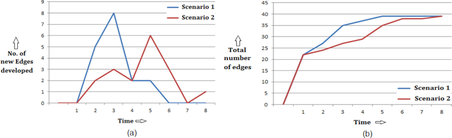
Variation of clustering coefficient for scenario 1 and 2.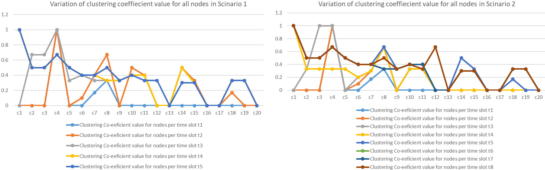
The authors have found out the clustering co-efficient for the 20 nodes from the graph that was considered for the theoretical explanation of the above link generation algorithm in Fig. 7. It was found that although the value of
Comparison of change in clustering co-efficient value for two different scenarios.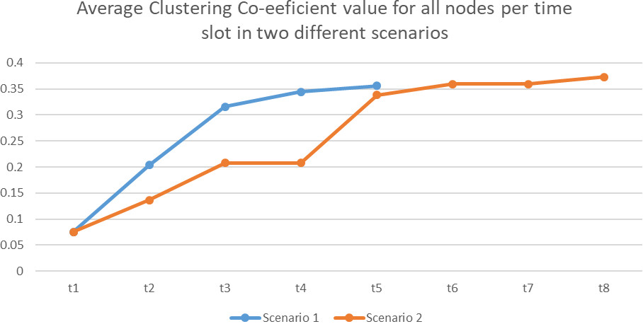
In order to have a deeper insight into the value of clustering coefficient, the average
Observation of degree centrality value for all 20 nodes for Fig. 9 in scenario 1 shows that the
Comparison of change in Degree Centrality value for two different scenarios.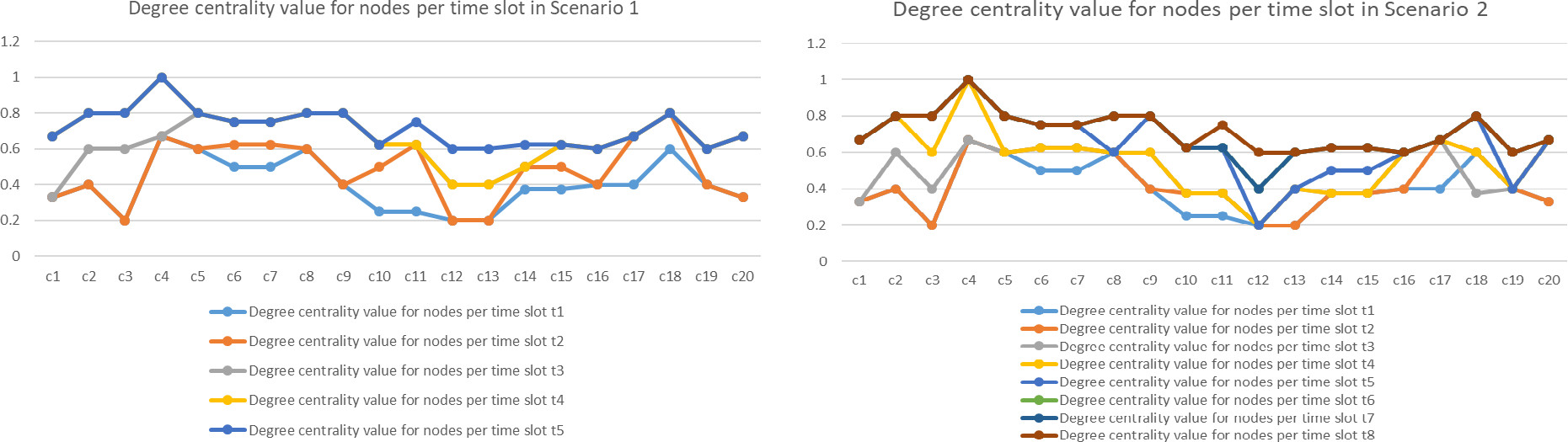
Comparison of change in average centrality distribution for two different scenarios.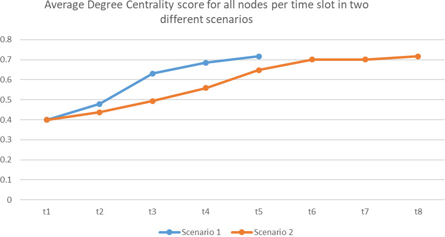
The same trend of incremental nature was observed for average centrality distribution for the successive time clots in both scenarios in Figure 10. The rise of the average degree centrality score was more for scenario 1 than for scenario 2 during initial time slots. This nature was observed till t5 i.e the time till scenario 1 was considered. After t5 the growth of the average centrality value for scenario 2 was not that much and was found to be almost constant during the final three time slots.
Description of the dataset
In order to implement the proposed algorithm and to check its effectiveness with the earlier approaches, the authors have used Stanford University dataset named as Arxiv HEP-TH (high energy physics theory) citation graph is from the e-print arXiv that covers all the citations within a dataset of 27,770 papers with 352,807 edges. If a paper
Since the data set is too large the authors have considered three different discrete portions for the implementation of the proposed DVNN-LPA. The first portion consist of the 1st 100 edges, the 2nd portion consist of the edges numbered from 17500 to 17620 while the last portion consist of the edges numbered from 34890 to 35000. Besides the dataset that has been considered consist of an un-directed graph without any edge length or weight thereby some portions of the algorithm that deals with the estimation of new edges on the basis of weights or edge length has not been considered. All the other notions as described within the algorithm has been taken into consideration for the implementation. Besides a square grid consisting of 10
The Authors have also considered a real and toy network datasets i.e 26KeroNetwork [31] that maps the favor exchange network in a rural village in India. The network consist of 135 nodes and 251 weighted edges. This dataset is considered for the implementation of all the criterias that was not possible in implementing in the previous dataset. For the sake of simplicity, the Manhattan distance of 1 is only taken into consideration.
Comparison parameters used
Demonstration of clustering coefficient.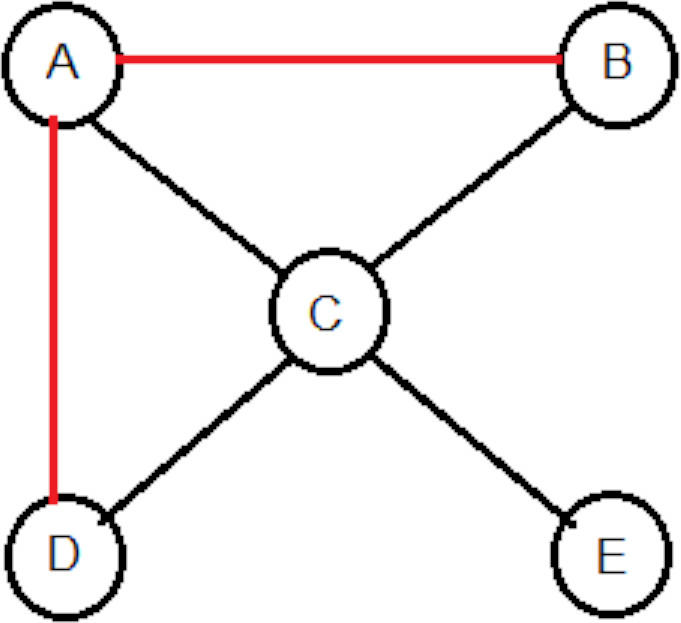
For the purpose of comparison with the earlier approaches, the following parameters were taken into consideration:
Clustering coefficient, concerns to the fact that for any node how many neighbors are connected. Therefore, it can be defined as a degree to which neighbors of a given node are linked to each other. It is defined by the formula:
Initially, in Fig. 11 Clustering Co-efficient for node
Degree centrality distribution. The degree of a node is the number of neighbors that it has. The degree centrality is the number of neighbors divided by all possible neighbors that it could have. Depending on whether self-loops are allowed, the set of possible neighbors a node could have could also include the node itself.
Jaccard coefficient value which is calculated as the common neighbors divided by the total combined neighbor nodes.
The Adamic-Adar index that has been an important parameter which predicts links in a social network based on the number of shared links between two nodes. It is characterized as the total of the invertible logarithmic degree centrality of the two nodes’ common neighbors.
The term “preferential attachment” refers to the fact that the more tightly attached a node is, the more probable it’s going to obtain additional links. Higher degree nodes have a greater capacity for attracting links to the network.
The diameter of a graph is the greatest distance between two vertices. Average diameter measures the maximum distance between each pair of vertices in the graph.
A graph’s effective diameter deff (G) is the minimum number of hops required for 90% of all attached pairs of nodes to access each other.
The average amount of edges along the shortest route for all possible combinations of nodes in the network is described as the graph’s Average Path Length (APL). Determining
Sample output for Successive time intervals obtained on implementing the proposed algorithm for the 1st 100 edges of dataset.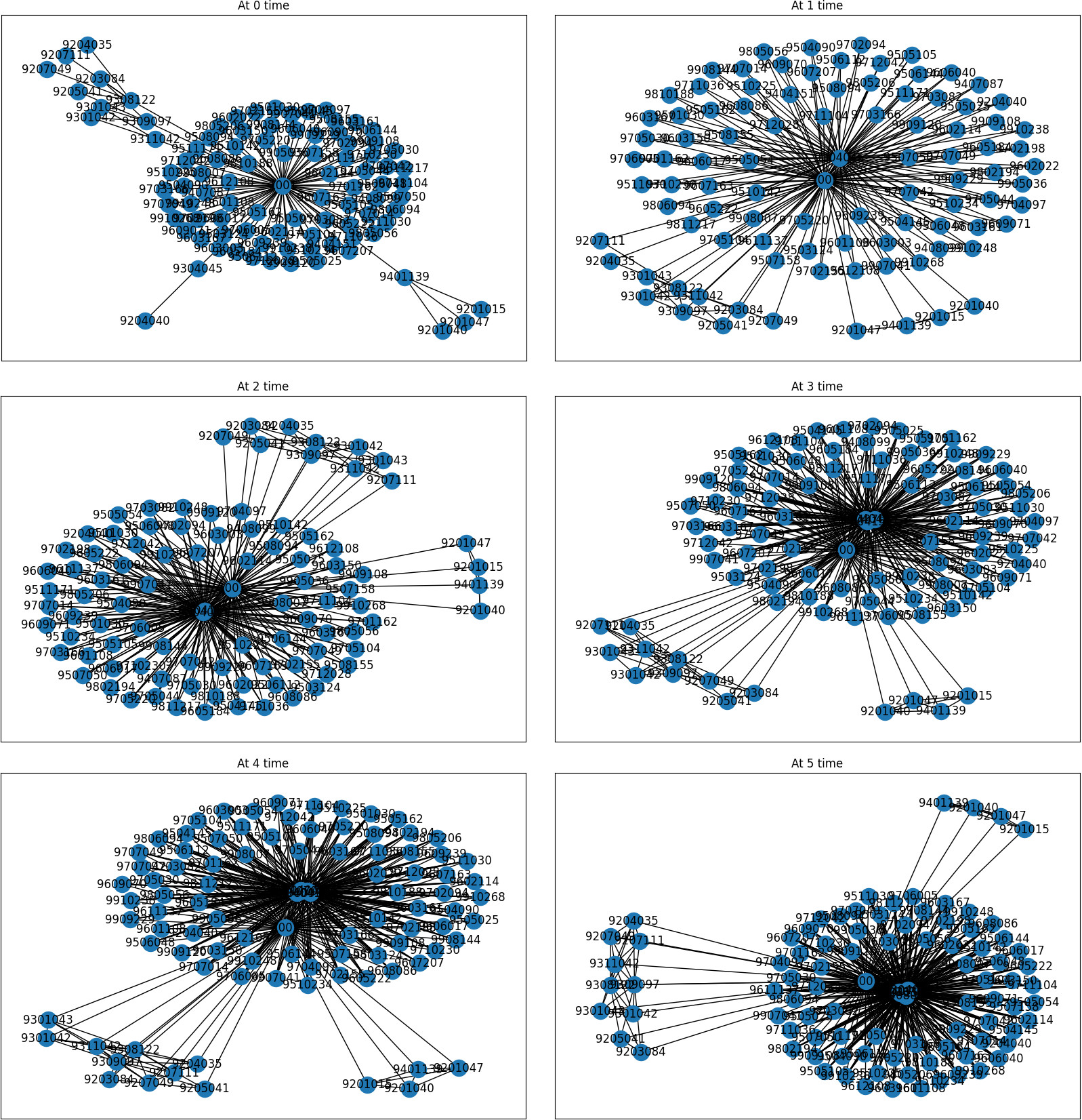
Arxiv HEP-TH dataset that has been considered is a huge dataset consisting of more than 35,000 edges, thereby taking the entire dataset and implementing the proposed DVNN-LPA is a huge task. Thereby to simplify the process, we have considered a collection of edges at three different instances. Initial 100 edges were considered primarily for implementation, thereafter two more instances i.e 120 edges from the middle of the dataset has been considerable. Finally, the 110 edges from the final part of the dataset has been considerable for study and analysis. The following screenshots in Fig. 12 shall demonstrate the sample output obtained on implementing the proposed algorithm for the 1st 100 edges on the Arxiv HEP-TH dataset. It will be seen that there is continuous development of edges obtained for each successive time slots. To verify the applicability of the algorithm various parameters have been extracted out for the successive time slots which will be demonstrated in due time.
The value of the different parameters for the 1st 100 edges obtained from the Arxiv HEP-TH dataset after algorithm implementation for six successive time slots, have been summarized in Table 1.
Parameter values for 100 edges obtained from the 1st portion of the Arxiv HEP-TH dataset
Comparison of the average parameter values. (a) Jaccard coefficient, Adamic Adar index, degree centrality and clustring coefficient, (b) preferential attachment and (c) average path length, diameter, average effective diameter obtained while implementing the proposed algorithm for the 1st 100 edges of Arxiv HEP-TH dataset.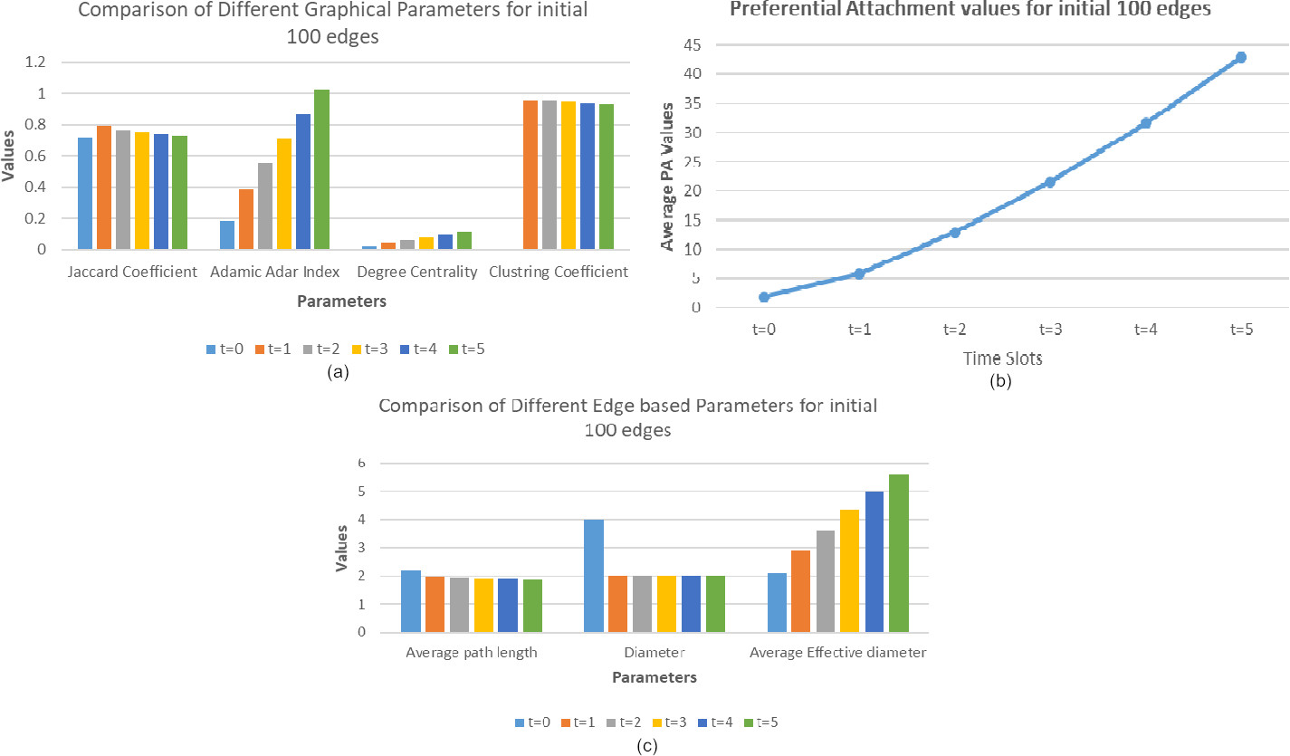
Based on the data of the parameters obtained, an analysis has been carried out. Figure 13 will demonstrate the fact.
Comparison of Graph obtained while implementing DVNN-LPA for the middle 120 edges of Arxiv HEP-TH dataset.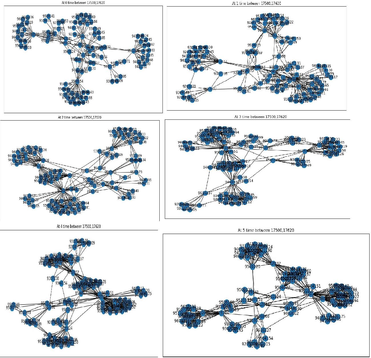
Figure 13a demonstrates the fact that value of the Jaccard coefficient value is found to be incrementing for the 1st time slot and this has successively reduced for the subsequent time intervals. But the reduction in value was very minimum and is almost ignorable considering the fact that a large number of edges is being added in subsequent time intervals. The value for Adamic-Adar index is also found to be increasing in successive time intervals because as more and more links are added in the network, and graph becomes dense, thereby increasing the value. Figure 13b shows that Preferential attachment value with the attachment of additional links with each time interval, the value has increased. Figure 13c shows the increase in the average degree centrality value of all nodes within the network verifies the fact that each of the node has become dense in subsequent time intervals. A constant diameter of 2 is observed within the graph for each time slots. Since the graph has become dense with addition of edges in each time slot, this value is incremental in nature. The APL value for the graph has almost remained the same for each time slots as the graph has no deletion of edges. The clustering coefficient value has almost remained constant throughout the time intervals and has no effect on the overall configuration of the graph.
Parameter values for 120 edges obtained from the middle portion of the Arxiv HEP-TH dataset
Comparison of the average parameter values. (a) Jaccard coefficient, Adamic Adar index, degree centrality and clustring coefficient, (b) preferential attachment and (c) average path length, diameter, average effective diameter obtained while implementing the proposed algorithm for the middle 120 edges of dataset.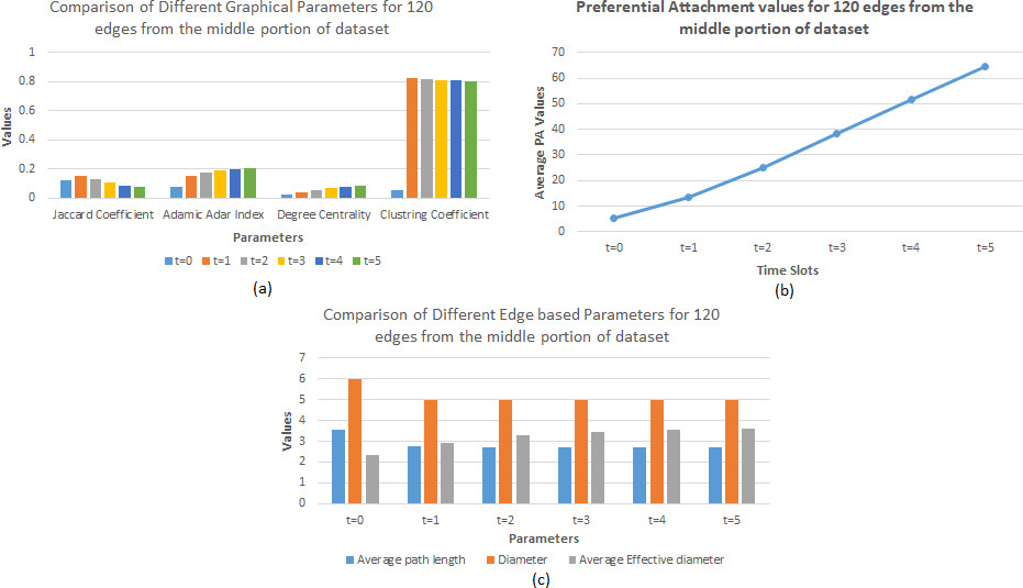
In the second instance, middle 120 edges i.e within the edge 17500 to 17620 of Arxiv HEP-TH dataset has been considered for parametric analysis. Figure 14 has been obtained at initial
The parametric values from the dataset after algorithm implementation for six successive time slots, have been summarized in Table 2.
Based on the parameter data obtained, an analysis has been carried out. Following Fig. 14 will demonstrate the analytical comparisons being made.
Figure 15a demonstrates the fact that Jaccard coefficient value has initially increased but has slightly decremented in further time slots. Adamic Adar index has incremented in each of the time slots as new graphs are attached. The values of preferential attachment have stiffly increased subsequently in Fig. 15b. All other parameters that includes degree centrality, average effective diameter and clustering co-efficient has also found an increment in each of the time intervals due to the addition of new edges in the graph. Within Fig. 15c decrement was only found in the value of average path length value, although this decrement was not that much and is almost countable to be constant. Diameter has maintained a constant value of 5 in each of the time intervals.
In the final instance, 110 edges i.e within the edge 34890 to 35000 of Arxiv HEP-TH dataset has been considered for parametric analysis. The value of the different parameters for the last 110 edges obtained from the Arxiv HEP-TH dataset after algorithm implementation for six successive time slots, have been summarized in Table 3.
Parameter values for 110 edges obtained from the final portion of the Arxiv HEP-TH dataset
Based on the values of different parameters, analysis will be carried out. Following Fig. 15 will briefly summarize the comparisons being made.
Comparison of the Average parameter values. (a) Jaccard coefficient, Adamic Adar Index, degree centrality and clustring coefficient. (b) Preferential attachment obtained while implementing the proposed algorithm for the 110 edges from last portion of Arxiv HEP-TH dataset.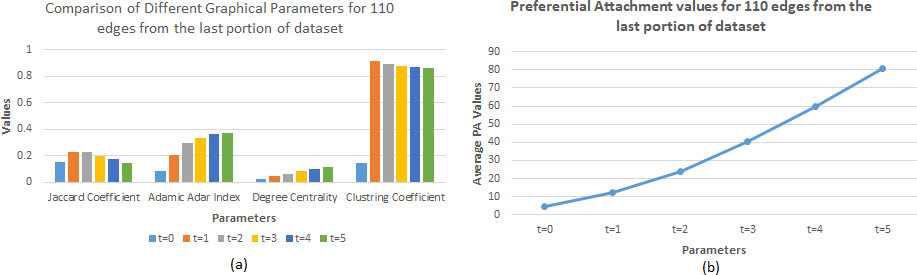
Comparison of the Total number of Edges developed while implementing the proposed algorithm for different instances of Arxiv HEP-TH dataset.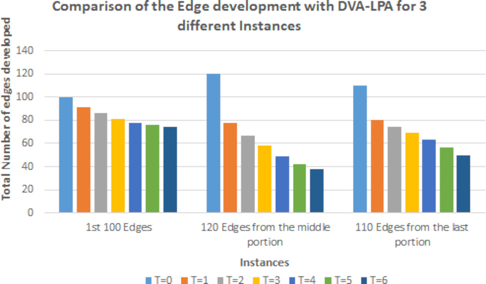
The graph above shows that in Fig. 16, the Jaccard coefficient value gradually increased but then declined slightly in subsequent time slots. As fresh edges are attached, the Adamic Adar index has increased across all time slots. Consequently, preferential attachment values have increased sharply. Most other parameters, such as degree centrality and clustering co-efficient, have increased across all time frames as a consequence of the addition of new edges to the graph.
The researchers have also made a comparison of the number of edges developed per time slot with the application of DVNN-LPA. Figure 17 shows that with each time slot, the number of edges being developed has decreased. This trend of decreasing nature of the total number of edges developed is viewed throughout the three different ranges. It will further decrease if more time intervals will be taken into consideration.
Parameter values generated for subsequent time slots while implementing DVNN-LPA on Real and Toy Network dataset
Comparison of Graph obtained while implementing DVNN-LPA on Real and Toy Network dataset.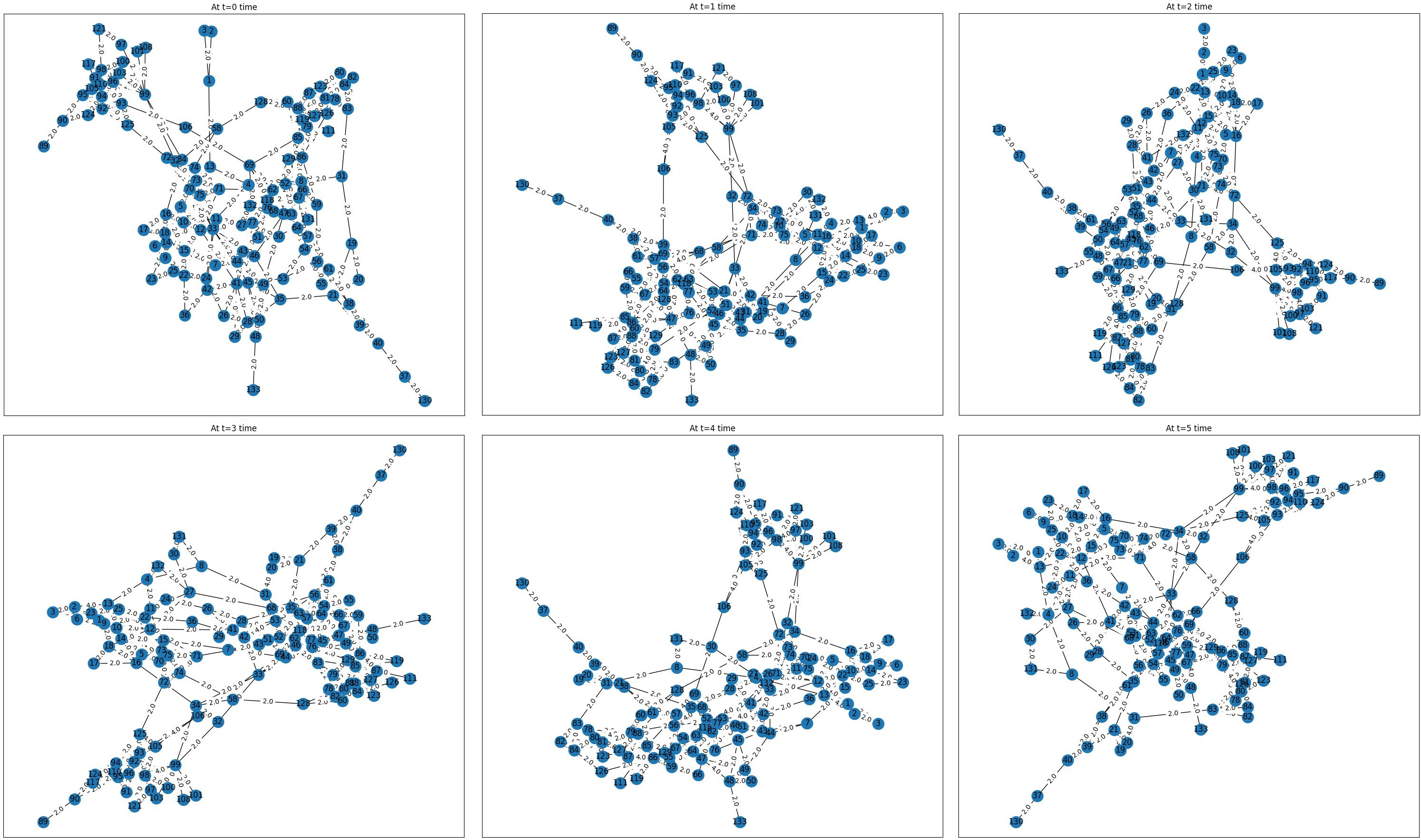
The proposed DVNN-LPA was also implemented on the Real and Toy Network Dataset and the outputs obtained for some subsequent time slots has been illustrated in Fig. 18.
On the basis of the Graph obtained in Fig. 18, an in-depth analysis is carried on the different parametric values and the following results as described in Table 4 was obtained.
Based on the values of different parameters, analysis will be carried out. Figure 19 will briefly summarize the comparisons being made.
Comparison of the average parameter values. (a) Graphical parametr values. (b) Edge based parameters. (c) Preferential attachment obtained while implementing the proposed algorithm for the Real and Toy Network dataset.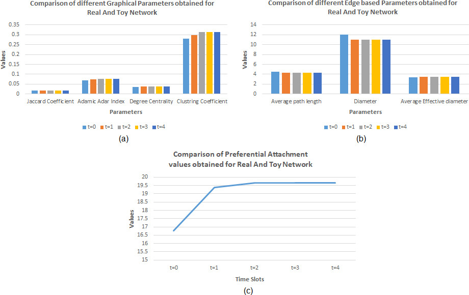
Figure 19a shows that very small incremental nature was found within the values of the Jaccard Coefficient and Degree Centrality, while the increment was slightly higher for subsequent time slots in the values of Adamic Adar index and Clustering Coeffiecient. On comparison of the edge based parameter values in Fig. 19b, it was found that very very less decrement was found within the values of average path length and diameter while the average effective diameter values has shown a little incremental nature. The values of the preferential attachment has shown an incremental nature and finally comes to a constant value in the final time slots as shown in Fig. 19c.
In order to verify the appropriateness of the Proposed DVNN-LPA with earlier approaches, several comparisons were drawn. Within [7] comparison was done on the basis of Average diameter of the undirected network over time. The diameter of a graph is defined as the largest shortest path distance in the graph. In other words, it is the maximum value of
Within [11], Average and effective diameter of the giant component of Flickr and Yahoo! 360 timegraphs, by week. A graph method that returns the (approximation of the) Effective Diameter (90-th percentile of the distribution of shortest path lengths) of a graph (by performing BFS from NTestNodes random starting nodes). This has been demonstrated in Fig. 20a, b and c respectively.
The increase in average effective diameter was observed for subsequent time slots throughout the time slots in both the ranges with an application of DVNN-LPA within Fig. 21a and this behavior is similar to the one that was observed in [7, 11]. The diameter also shows a uniform trend in subsequent time slots both for flickr and yahoo 360 and such a similarity was observed in DVNN-LPA where a uniform trend in diameter was observed for subsequent time slots in Fig. 21b. Therefore, a conclusion can be drawn that DVNN-LPA is very much efficient as compared to the earlier approaches.
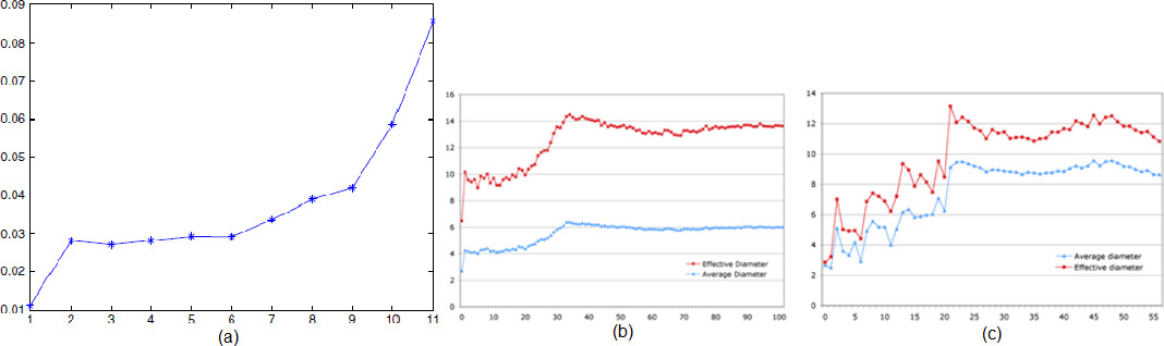
(a) Diameter and effective diameter obtained with the application of DVNN-LPA for the 1st 100 edges. (b) Diameter and effective diameter obtained with the application of DVNN-LPA for the 120 edges from the middle range.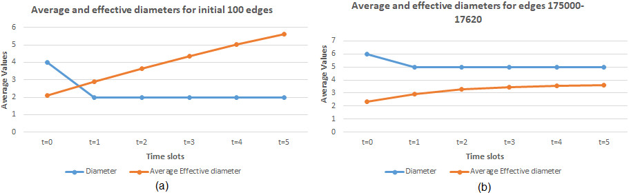
(a) Clustering coefficient and (b) degree centrality value for nodes as described for flickr dataset in [12]. Distribution of (c) clustering coefficient and (d) degree centrality value for initial 100 nodes for respective time slots with DVNN-LPA.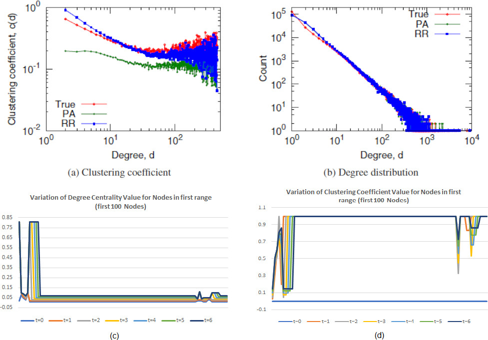
As illustrated in [12] ie Fig. 22a and b during first process (PA), selection of node is done preferentially, with probabilities proportional to their degrees for edge addition. Then during the next process (RR), random-random triangle-closing model has been used, where a node is selected at first preferentially and further a selection of a node that is located two hops away with the usage of random-random model is being done. While during the application of DVNN-LPA, selection of node is done within the Von-Neumann neighborhood having a Manhattan distance of 1. This process is repeated consequently for the selection of new nodes within the same neighborhood. Figure 22c and d has demonstrated the fact that how the clustering coefficient and degree centrality value has incremented for subsequent time slots for each of the nodes.
(a) Comparison of new edges developed for different Dataset with GERM algorithm as described in [14]. (b) Comparison of new edges developed for three different Intervals of the ArXiv dataset with DVNN-LPA.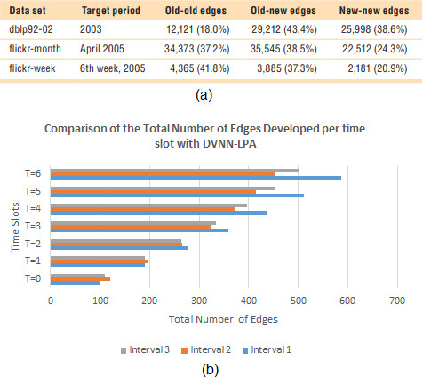
As discussed in [14] the Table within Fig. 23a provides data analysis on the target prediction time frame that has been used in the experiments based on three different data sets. The table specifically indicates the quantity of edges connecting two old nodes (that is, nodes that was present during the training period), one old and one new node (old-new), and two new nodes (new-new). The old-old categories involve cases which can be managed by both traditional link prediction as well as our framework; the new-old category involves cases that our method is capable of handling but traditional link prediction cannot. Neither the given GERM Algorithm framework nor the traditional link prediction framework is capable of handling the new category. As shown in the above Table within Fig. 23a, the old-new category accounts for a large proportion of freshly generated edges across all data sets. While comparing the results in Fig. 23b, it was found that the average growth rate of 36.5%, 27% and 30.4% respectively was found for each of the three different intervals for the Proposed DVNN-LPA while the results for dblp 92-02, flickr-month and flickr-week shows the growth rate was 33.3% for the specified period. The results were quite comparable and would have been further increased if long intervals were considered for the study in implementing DVNN-LPA.
Let us consider the case of 20 students who are admitted to the first year of a Bachelor of Engineering course at a university. Their first day of university is considered time t=0. During the period, only two students were associated as they were from the same school. No other kind of association exists between the students as they are fully unknown to each other. Very few associations are found to exist among them at the end of their first semester (
Conclusion
Over the last two decades, social networks have gained enough popularity and have succeeded enough in order to create efficient communication among people. This usefulness has attracted researchers in their investigation of the possible ways of modeling social networks. Usage of static methods in modeling the dynamism of social networks is a challenge. The authors discuss the applicability of neighborhood theory for modeling dynamic social networks throughout the paper. As far as the knowledge of the authors in addition to the literature survey being presented within the paper, this model is the first attempt in modelling network with conception of neighborhood concept of cellular automata. This type of automata has been a significant tool in numerous applications and has remained to be ignored in the domain of modelling a network. This study shall present the initial attempt in simulating a developing network. Although various link prediction approaches have been discussed previously by various researchers considers time bound functionalities or various higher ordered features of graphs, but an integration of some of the basic graphical features with the neighborhood conception of cellular automata has not been done. To this an extent, the modelling and the link prediction approach that has been presented within this paper is novel in nature. It has also been shown that the proposed link prediction algorithm works better than the previously proposed approaches in terms of the applicability through theoretic and programming simulations. Future work regarding the same will involve the applicability of the method and the algorithm on the real-world dataset for observing the growth of the network for each year considering it as a larger snapshot that will include several smaller snapshots of whenever a new link appears. It has also been shown that the proposed link prediction algorithm works better than the previously proposed approaches in terms of the applicability of a real-life problem.
Footnotes
Conflict of interest
The authors declare that they have no known competing financial interests or personal relationships that could have appeared to influence the work reported in this paper.