An effective deep learning model with reduced error rate for accurate forecast of stock market direction

Abstract

Prediction using ML models is not well adapted in many portions of business decision-making due to a lack of clarity and flexibility. In order to provide a positive risk-adjusted price for stocks by evaluating historical transaction data and retaining more accuracy with a reduced error rate, the suggested framework aims to use deep learning method. The deep learning methodology, which can handle time-series data, is applied in this work. The measurements of MSE and RMSE error rates, which indicate how far the measured values are from the regression line, are used to produce the findings. The dispersion of these residuals is evaluated by RMSE. It demonstrates how densely the data is clustered around the line of best fit. In this work, a novel deep learning approach is compared to deep LSTM, GA, and Harris Hawk optimization. Outcomes were obtained and exhibited for the various firm stocks dataset as part of this investigation, which amply demonstrates the usefulness of the proposed strategy with a lower error rate.

Keywords

Stock market prediction recurrent neural network deep LSTM deep RNN deep learning optimization

1. Introduction

Wealth and commodities could be able to provide us a comfortable and secure way of life. It makes sense that there is so much interest in the research and forecasting of potential financial market values and estimates. Numerous forecasting strategies have been proposed and employed. Each technique has advantages and disadvantages of its own. Additionally, as online trading has grown in popularity, amateur investors have turned to the stock market to make big profits. Therefore, it would be very tempting if the framework could accurately predict market behavior so that investors could make informed investment decisions. Due to the significant implied volatility rules influencing price movement, developing such a forecasting model is a difficult task.

Due to its ability to deal with ambiguous, imperfect, or insufficient data that varies often in very short timeframes, neural networks (NNs) have emerged as a crucial instrument for stock price forecasting [18]. These study’s objectives include highlighting the issues that require more exploration in research as well as outlining the key benefits and drawbacks of earlier approaches used in RNN applications for the stock market. A comparison of preceding research’s technique in terms of challenge domain, data models, and outcomes criteria led to the discovery of several advantages and limitations. Numerous complex events, such as economic cycles, warning tactics, interest rates, political ideologies, etc., may have an impact on the stock exchange. There are several forecasting strategies, but the majority of them each have benefits and drawbacks of their own. Common mathematical methodologies must be used in conjunction with the underlying seasonality, non-stationarity, and other characteristics in specific [19]. Additionally, using standard statistical methods without specific understanding becomes problematic. The main goal of financial forecasting is to pinpoint trend lines, which enables investors to stick to their investment strategy till confirmation demonstrates a change in the trend. Two of the most fundamental and well-known trading ideas, the moving average and trading range break-out criteria, were originally studied in [20]. For decision-makers in many domains, improving forecasting accuracy, especially for time series predictions, is an important and difficult problem. There is always room for improvement in predicting prediction accuracy. Despite the large number of time series models at the moment. Time series forecasting models discover that combining forecasts from several models typically results in improved performance, even when the models in the ensemble are substantially different from one another [21]. Artificial neural networks (ANNs) have proved effective in pattern recognition, classification, grouping, and forecasting with enhanced accuracy [22, 23, 24]. The toughest task in time series prediction is sometimes thought to be forecasting. Due to the noisy character of the information used, the forecast for the time series trend of the financial market is less precise. According to the efficient market hypothesis (EMH), it is impossible to predict future prices using the performance of financial assets since excess returns are always zero. This is so because the distribution function of a financial time series suggests a Brownian motion, which has characteristics of an independent, random, and Gaussian distribution. Some study, on the other hand, disagrees with EMH and believes that there is a recurrent pattern that might help anticipate future values. Over the past few decades, there has been a surge in the use of ANN and SVM for financial time series prediction [25]. These applications of ML models improve the forecasting accuracy of financial time series. This study focuses on the data preprocessing and data augmentation approach to make data more noise-free and consistent while analyzing the prediction performance of an enhanced form of LSTM that works with recurrent neural network. Finally the findings for various time series data are obtained and evaluated by the Root Mean Square Error (RMSE) and MSE measure. The conclusion is obtain after analyzing the RMSE & MSE results of each dataset and analysis proves that proposed architecture is proven to be effective in reducing the error rate and forecasting the future price direction up to a year.

2. Literature review

2.1 Approaches

The literature overview of conventional stock market forecasting methods is described in this part, along with discussions of their advantages and disadvantages. This information inspires researchers to develop a feasible stock market forecasting method.

A method used in artificial intelligence called machine learning (ML) that enables a system to learn from experience and make predictions without the need for precise scripting [8]. Several ML algorithms have already forecast the behavior of the market. Several researchers have applied neural network models extensively. The four main categories of contemporary stock analysis and forecasting techniques are sentiment analysis, machine learning (ML), pattern recognition, and statistical analysis. Market trends have also been predicted using time delay analysis. SVM,Bayesian belief networks, and evolutionary algorithms are a few examples of machine learning algorithms [17]. Machine learning techniques like the k-NN regression model assert that it is more accurate than other regression methods like linear regression and SVM. Stock price forecasting has already been attempted, but only for financial advantage under the pretext of computer trading. Candlestick analysis is a common stock market pattern that predicts stock open and closing values based on preceding and historical data [8]. In comparison to the quantity of literature based on daily close data, the authors Martinez et al. (2009) demonstrate that using an artificial neural network (ANN), they can estimate the lowest and highest stock prices of the current trading day of the two leading stocks on the Brazilian stock exchange [26]. Mettenheim and Breitner (2012) demonstrate that using ANN model predictions, it is able to correctly estimate the intraday dynamics of five liquid US equities [27]. Adebiyi et al. [28] evaluate the predicting accuracy and comparison of the NYSE Exchange’s multi-layer perceptron model’s accuracy to an ARIMA model. They found that, in terms of mean squared error, the MLP model performed better than the ARIMA model. Owing to significant developments in deep learning techniques, In recent years, a number of applications including natural language processing, speech recognition, and computer vision have identified RNN as a viable model for managing linear data. Furthermore, several research demonstrated that RNN with LSTM cells is the most effective model for predicting financial time series. For example, Chen et al. [29] proposed an LSTM-based stock price prediction model. Many fundamental stock variables are regarded as input characteristics. The model was evaluated on an additional 311361 samples after being trained on 900000 samples. They found that LSTM might do well in projecting changes in China’s index prices. In prediction accuracy, the experimental findings showed that their approaches beat the regression model of ordinary least square. Although MLP may be used to predict time series models, multiple research have shown that it has certain limitations in learning patterns since stock data has a high dimension and a lot of noise. On outliers, MLP frequently demonstrates uneven and variable efficiency [30].

Long et al. [31] evaluated a DNN framework employing open market data and transaction histories to evaluate price direction. Their final study revealed that bidirectional LSTM achieved the best outcome and could estimate the growth of the market for investors. Rekha et al. [32] looked at how RNN and CNN algorithms were used and contrasted their accuracy with actual stock market data. To provide more precise stock market forecasts, Pang et al. [33] merged LSTM with an automated encoder and LSTM with an integrated layer. According to basis of empirical evidence The Shanghai Composite Index was produced with 57.2 percent accuracy using LSTM with an integrated layer. Kelotra and Pandey used the deep convolutional LSTM technique to successfully anticipate changes in the stock market. RMSE and MSE were 2.6923 and 7.2487 respectively, using a Rider-based monarch butterfly optimization approach [34].

In this study, comparison is carried out for the accuracy of three machine learning models (Harris Hawk optimization, GA and Deep LSTM) with proposed model in predicting stock price movement. Our model receives seven derived technical indicators as input. Model employ stock market data (open, close, high, low, and spread values). Data is augmented at the final stage of processing for input utilizing bootstrap approach. The data augmentation is used to minimize the over fitting issue and also enhances the generalization of systems. The bootstrap approach is used here as a kind of re-sampling technique. Based on the underlying characteristics of the market, each technical indicator has a distinct potential for upward or downward movement. The effectiveness of the cited models all experimental tests are performed using historical data from three market equities from various industries (FMCG, communications, and automobile) that encompass three, five, ten, and twenty years.

2.2 Challenges

Analysis and forecasting of the stock market remain complex and fascinating issues. Because more information becomes accessible, collecting and analyzing it to extract insights and assess market pricing presents new hurdles. Determine the performance criteria for erratic trend changes. The examination of all these techniques and performance provides even another issue since new learning models frequently enter the market. As these represent the prospective rate of returns, time series behavior of mispricing in the Indian market has to be studied. Literature also provides evidence of seasonal abnormalities in stock return series. It has to be investigated if shifting market circumstances and other variables affect the flow of knowledge.

It is necessary and overdue to examine the information flow between price and trading activity variables together since doing so would include a larger market and give a clearer picture of future price behavior. Scaling is required since the current system requires some sort of input interpretation. The prior findings suggest that when the conventional classifier is applied, the stock price is uncertain. Some neural network approaches have slow convergence rates a neural network takes longer to train because of its complexity. It is difficult to determine the global minimum and maximum because local neural minima and maxima networks, which rely on gradient descent approaches to discover local maxima, tend to get stuck on local minimum and maximum. Each machine learning method has its own advantages and disadvantages and is only useful under certain conditions. Although financial time series are not linear, a number of statistical assumptions, such as linearity and normality, have been made in the methodology. As a result, these strategies are ineffective for predicting stock prices. Fundamentals analysis performed automatically is not without flaws. First off, there is no assurance that there will be no disinformation, even if statements or reports are released by businesses, the media, or some other independent organization. It is unclear how much disclosure and stock price volatility are correlated.

Forecasting is a difficult task since stock time series data is dynamic and complicated. It is so challenging to use a range of deep learning algorithms for both sentiment feature engineering and stock movement prediction modelling. A variety of financial time series may be predicted using the hybrid forecasting paradigm. For accurate stock market forecasting, the forecasting findings may be integrated in effective stock market monitoring and financial data analysis [2]. Improved quality outcomes for forecasting will be obtained by using a more methodical approach to selecting stock-relevant keywords for social media and news monitoring [6].

3. Proposed method

Figure 1.

Block diagram of proposed method.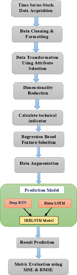

The purpose of the study is to evaluate and compare the performance of three existing methods Harris Hawk optimization, GA and deep LSTM with improved proposed framework improved recurrent rider deep LSTM (IRRLSTM). Here experiment is conducted without using any optimization techniques to train the proposed model. Step by step block diagram of experiment is shown as follows. Detail of procedure is discussed in further subsections.

3.1 Acquisition of input data

This study will be based on historical time series data that spans three stock market sectors (FMCG, communications, and car) throughout periods of three, five, ten, and twenty years from 2010 to 2020. Seven technical indicators are chosen for this study in order to save calculation time. There are several technical indicators available for forecasting stock market movement, and each has a distinct ability to predict future market moves. Technical indicators including the Average True Range (ATR), Triple Exponential Average (TRIX), Rate of Change, Relative Strength Index, Average Directional Movement Index, and William’s Percent Money Flow Index are utilized in this model to extract the features. Then, using a regression-based feature selection wrapper approach, the feature vector acquired from the feature extraction phase is put through the feature selection process. Additionally, the chosen feature is fed into the stage of data augmentation using the Bootstrap approach. Finally, an enhanced Recurrent Rider LSTM is suggested and used to identify stock market activity. However, the suggested enhanced Recurrent Rider LSTM is created by fusing Deep RNN and Rider Deep LSTM.

3.2 Data preprocessing

As the time series data is obtained from online web resource, gathered data consist of some irrelevant and noisy values which need to be preprocessed before using as an input to the proposed framework. Real-world data typically includes noise, missing values, and may be in an undesirable format, making it impossible to build machine learning models on it directly. Pre-processing data is required to clean it and prepare it for a machine learning model, which also improves the model’s performance and robustness. In this research, the mean values of the property are used to replace NULL and missing values.

3.3 Feature extraction

To extract pertinent and desirable features, the input was exert for the feature extraction process. The process of constructing a new feature space, known as feature extraction, is regarded as a crucial component for classification and analysis purposes. It is necessary identify independent, fundamental, technical, and macroeconomic elements for forecasting stock. Model basically attempt to extract fundamental variables like open, close, High, Low, Volume, etc. A crucial role in distinguishing the features from a given dataset is played by the technical indicators. It was able to make effective predictions as a consequence. Seven technical indicators are used in this model to extract the characteristics, which are described below.

3.3.1 Average true range (ATR)

The volatility is assessed using the ATR, or average true range. Additionally, it is used to assess the length of time.

$\displaystyle f_{1}=a(f_{1_{\textit{ran}}},n)$

where $a$ denotes ATR, and $f_{1_{\textit{ran}}}$ specifies the true range.

3.3.2 Rate of change (ROC)

The momentum indicator is another name for the ROC indicator. It is used to calculate the current and historical prices for specific time intervals.

$\displaystyle f_{2}=\frac{I(k)}{I(k-n)}*100$

where, $I(k)$ implies the latest price and value of a limited number of period is signified as $I(k-n)$ .

3.3.3 Relative strength index (RSI)

The RSI is a momentum oscillator used in order to ascertain whether a product is overbought or oversold.

$\displaystyle f_{3}=\frac{A_{v}(P_{u})}{\left(A_{v}(P_{u})+A_{v}(P_{d})\right)% }*100$

where,

$\displaystyle\begin{cases}P_{u}(k)=1*(P(k)-P(k-1)),&\textit{for}\ P(k)-P(k-1)>% 0\\ P_{d}(k)=1*(P(k-1)-P(k)),&\textit{for}\ P(k)-P(k-1)<0\end{cases}$

where, $A_{v}({P_{u}})$ indicates the average of price up value and mean of price down value is specified as $A_{v}(P_{d})$ .

3.3.4 Average directional movement index (ADMI)

The Average Directional Movement Index (ADMI) measures the strength of a trend, which is determined over past 10 days corresponding to the input window length. It also indicates about the trending and non-trending condition of a market.

$\displaystyle f_{4}=100*\frac{(\textit{DI}^{+}-\textit{DI}^{-})}{(\textit{DI}^% {+}+\textit{DI}^{-})}$

3.3.5 William’s % R

In addition to being an inverse of the Fast Stochastic Oscillator, an indication of momentum is William’s percent R. The ratio of the change in the difference between the highest and nearest price to the change in the difference between the highest and least price is known as William’s percent R.

$\displaystyle f_{5}=\left[\frac{(H_{p}-C_{p})}{(H_{p}-L_{p})}\right]*100$

where, $H_{p}$ and $L_{p}$ denotes the highest and lowest price, respectively. The closest price of the current day is represented as $C_{p}$ .

3.3.6 Money flow index (MFI)

The level of the money supply is assessed by the Money Flow Index and establishes the selling and purchasing pressure using both price and volume.

$\displaystyle f_{6}=\left(100-\frac{100}{(1+M_{r})}\right)$

where, $M_{r}$ denotes the Money ratio.

3.3.7 Triple exponential average (TRIX)

The triple exponential moving average is a tool for facilitating insignificant fluctuations. The TRIX indicator is notated as $f_{7}$ .

The aforementioned seven feature vector is produced by combining features, and the extracted feature is shown as,

$\displaystyle f=\{{f_{1},f_{2},f_{3},f_{4},f_{5},f_{6},f_{7}}\}$

3.4 Feature selection

A fundamental stage in the realm of stock market forecasting is feature selection in which pertinent variables are chosen in accordance with their importance. It is also more beneficial in lowering the dimension size of the datasets to increase the precision and effectiveness of prediction systems. Characteristics that are unimportant or just marginally significant might harm a model’s performance. Regression-based feature selection is used in the experiment. In this wrapper strategy, the evaluation function is the classifier error rate. To identify all the feature subsets, the classifier is wrapped in the wrapper technique. By learning the error rate and classification accuracy, the machine learning algorithms simplify the wrapping method to feature selection. Based on learning algorithms, it fine-tunes the prediction system. The wrapper approach’s key contribution is to lower classification error and improve classification performance.

3.5 Data augmentation

The technique of enhancing data by producing additional data that corresponds to the original data is known as data augmentation. Here, data augmentation is employed to improve system generalization and reduce the problem of over fitting. The bootstrap method is a type of resampling strategy used to sample a database using replacement and get statistics like mean or standard deviation. It is mostly used to assess the capabilities of machine learning models while generating predictions based on training data.

3.6 Cross validation

Cross-validation is a method to try to reduce overfitting (optimism) in a fitted model. By randomly splitting the dataset as above, the final model is less secure, but overall the process tells you something about how the model might be generalized to a new independent dataset. This is one way to perform model validation. Here in this study, we have used Leave-one-out cross-validation (LOOCV). It is an extreme case of $k$ -Fold CV. Imagine if $k$ is equal to $n$ where $n$ is the number of samples in the dataset. We have taken $n=$ 10.

Figure 2.

Rider Deep LSTM.

The algorithm:

Select a sample from the dataset that will be the test set.

The remaining $n$ $-$ 1 samples will be the training set.

Train the model on the training set. A new model trained for each iteration.

Validate on the test set.

Save the result of the validation results.

Repeat steps 1–5 $n$ times as for $n$ samples we have $n$ different training and test sets

To get the final score average the results got on step 5.

3.7 Proposed improved Recurrent Rider LSTM

Incorporating Rider Deep LSTM with Deep Recurrent Neural Network results in the proposed Recurrent Rider LSTM. In the part that follows, the structures of the Rider Deep LSTM network and Deep Recurrent Neural Network are briefly explained.

3.7.1 Rider Deep LSTM network

Rider Deep LSTM operates on time series data [34]. The Rider Deep LSTM’s main contribution is the function of memory gates and forget gates, which are used to manage information in order to rebuild appropriate information at all times. The core of the network’s four levels are input layer, fully connected layer, LSTM layer, and output layer for regression. The Rider Deep-LSTM updates the trained network up until the previous step while making predictions about the values at each step and being aware of data trends. Finally, the fault values are predicted using the trained network. Rider Deep-structure LSTM’s is as per shown in Fig. 2.

3.7.2 Deep RNN

RNN is a popular learning method that is also employed as an estimator and is very practical when dealing with time-series data. Large networks’ handling of temporal movement during the training phase is implemented by the RNN. RNN is a high throughput network structure that preserves the unprocessed sensor input without removing the feature and also offers high detection rates with quick sequential processing. An Elman-type network with a number of layers, such as the Deep RNN network, is one in which the internal layers are completely linked at the same network based on time direction. The Deep RNN network’s structure is shown in Fig. 3.

Figure 3.

Deep RNN.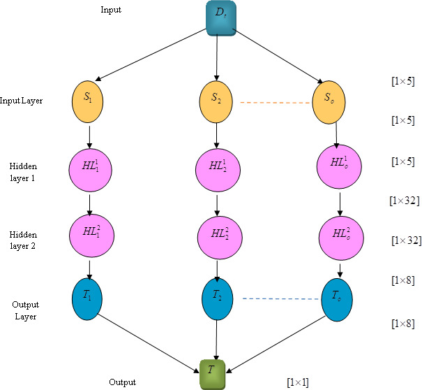

The input vector of $g^{\text{th}}$ layer at time period $x$ is given by,

$\displaystyle S^{(g),x}=\left[S_{1}^{(g),x},S_{2}^{(g),x},\ldots S_{y}^{(g),x}% ,\ldots S_{o}^{(g),x}\right]$

And the output vector of the $g^{\text{th}}$ layer at time x is expressed as,

$\displaystyle T^{(g),x}=\left[T_{1}^{(g),x},T_{2}^{(g),x},\ldots T_{y}^{(g),x}% ,\ldots T_{o}^{(g),x}\right]$

Here, $y$ is an arbitrary unit number of $g^{\text{th}}$ layer and $o$ represents the total count of units.

The previous hidden layer’s output is given as input for the next hidden layer, which produces an output with a dimension of [1 $\times$ 8]. Additionally, the output layer is sent to the output layer from the hidden layer, which creates a final output with a dimension of [1 $\times$ 1].

3.7.3 Algorithm for the improved Recurrent Rider based LSTM

#Algorithm for Rider based Deep LSTM Define Input: $D_{t}$ Define parameters for sigmoid activation function, bias of input gate, forget gate, and output gate previous time step: $j^{G},j^{F},j^{O}$

$\displaystyle\beta,q^{F},q^{G},q^{O},b^{G},b^{F},b^{O},b^{K},h^{t-1}$

Begin LSTM layer with input gate, Forget gate, output gate and memory cell: Define Time stamp $h^{t}=O^{t}\,\circ\tan l({K^{t}})$ Train Neural Network Append the optimal weights to the network Produce Output layer with linear regression layer End

#Algorithm for Deep Recurrent Neural Network Input: $D_{t}$ Input layer: $S_{1},S_{2},S_{o}$ Hidden layer 1: $\textit{HL}_{1}^{1},\textit{HL}_{2}^{1},\textit{HL}_{0}^{1}$ Hidden layer 2: $\textit{HL}_{1}^{2},\textit{HL}_{2}^{2},\textit{HL}_{0}^{2}$ Output layer: $T_{1},T_{2},T_{0}$ Output: $T$ Begin Calculate Input vector of $g^{\text{th}}$ layer at time period $x$

$\displaystyle T^{(g),x}=\left[T_{1}^{(g),x},T_{2}^{(g),x},...T_{y}^{(g),x},...% .T_{o}^{(g),x}\right]$

Calculate Output vector of the layer at time Train neural network: Begin Initialize weights If $i<i_{\max}$ Compute fitness function,

$\displaystyle\omega=\frac{1}{m_{i}}\sum_{jj=1}^{m_{i}}[\textit{XY}_{jj}-T_{y}^% {(g),x}]^{2}$

Build herd Calculate step size Calculate the solution vector Update the solution vector Compute $\gamma$ and $\phi$

$\displaystyle\gamma=\gamma_{0}-\frac{\gamma_{0}}{\max\ \textit{iteration}}% \times\textit{iteration}$ $\displaystyle\phi=\phi_{0}+\frac{\phi_{\max}-\phi_{0}}{\max\ \textit{iteration% }}\times\textit{iteration}$

If $i>i_{\max}$ End if Return optimal weights End Append the optimal weights to the network

4. Results and discussion

Table 1
MSE results of Asian Paints

Stock	Historical data duration (in years)	Metric	HHO	GA	Deep LSTM	Proposed model IRRLSTM
Asian Paints	20	MSE	0.611	0.598	0.514	0.067
Asian Paints	10	MSE	0.597	0.572	0.559	0.064
Asian Paints	5	MSE	0.619	0.598	0.504	0.066
Asian Paints	3	MSE	0.614	0.563	0.550	0.062

Table 2

MSE results of Bajaj Auto

Stock	Historical data duration (in years)	Metric	HHO	GA	Deep LSTM	Proposed model IRRLSTM
Bajaj Auto	20	MSE	0.602	0.579	0.546	0.06
Bajaj Auto	10	MSE	0.583	0.577	0.568	0.06
Bajaj Auto	5	MSE	0.582	0.581	0.565	0.06
Bajaj Auto	3	MSE	0.585	0.573	0.570	0.06

Three stocks from the NSE of the Indian stock market – Asian Paints, Bajaj Auto, and Bharati Airtel are used as a dataset with duration of three (from 2018 to 2020), five (from 2015 to 2020), ten (from 2010 to 2020) and twenty (from 2000 to 2020) years and downloaded from http://www.moneycontrol.com portal, with their attribute of Date, open, high, low, close, volume and Spread for testing and analyzing the proposed enhanced recurrent rider LSTM and existing approaches. The dataset attributes includes open, high, low, close, volume, and other technical indicators. MSE shows the root of the average squared difference between the actual values and projected values in a dataset, whereas the average squared difference between the actual values and expected values in a dataset is shown by RMSE. MSE and RMSE are regarded as assessment metrics. If a model has a lower RMSE value, it will be more accurate. To evaluate the consistency and effectiveness of the model, result graphs for MSE and RMSE are displayed for the three stock datasets over periods of three, five, ten, and twenty years of time series. Numerical results obtained of MSE & RMSE of mentioned stocks are tabularized from Tables 1–8 and same is depicted utilizing graphs in Figs 4–14 for better and effective empirical analysis and understanding of results, it also simplify complicated textual result description using concerned graph figures. Mapping of Tabular results into graph figures is to make quick understand and visualize results trends from result data. Respective result graphs figures are plotted to clarify, illustrate and augment the numerical results. Results for MSE of all three datasets are displayed in Tables 1–3 and results for RMSE are displayed in Tables 4–6. Empirical analysis of MSE results for the Asian Paints, Bajaj Auto, and Bharati Airtel is shown by Figs 4–6. Also analysis of RMSE for the Asian Paints, Bajaj Auto, and Bharati Airtel is shown by Figs 7–9. As shown in Fig. 4 results for the MSE of Asian paints for four methods, proposed model shows lowest MSE level of 0.062, Figure 5 shows results for the MSE of Bajaj auto for four methods, proposed model shows lowest MSE level of 0.06. Figure 6 shows results for the MSE of Bharti Airtel for four methods, proposed model shows MSE level of 0.08 which is lowest.

Figure 4.

MSE of Asian Paints.

Figure 5.

MSE of Bajaj Auto.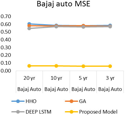

Similarly as shown in Fig. 7 results for the RMSE of Asian paints for four methods, proposed model shows lowest RMSE level of 0.24, Figure 5 shows results for the RMSE of Bajaj auto for four methods, proposed model shows lowest RMSE level of 0.248. Figure 6 shows results for the RMSE of Bharti Airtel for four methods, proposed model shows RMSE level of 0.29 to 0.31. In order to study the effectiveness of proposed LSTM model with respect to deep LSTM, results are plotted and observed in Figs 10 and 11 for MSE & RMSE. Collective results of all dataset for all-time series duration are plotted in Figs 12 and 13, which concludes that proposed approach is proved to be effective as compare to existing HHO, GA & deep LSTM methods.

Tables 1–6 values indicates the residuals’ standard deviation (prediction errors). It shows how closely the data are grouped around the line of best fit. Better fit is shown by lower MSE and RMSE values. A decent indicator of how effectively the model was used to determine the reaction is the RMSE. If the primary goal of the model is prediction, then this fit criteria is crucial.

4.1 Statistical test

A statistical test is performed for the comparison of the examined methods. We have utilized D’Agostino-Pearson normality test [35]. It is a measure of the goodness-of-fit of the deviation from normality, i.e. the test aims to measure the compatibility of given data with the null hypothesis that the data is a realization of independent, identically distributed Gaussian random variables. It is a versatile and powerful normality test. The test is based on transformations of the kurtosis and skewness of the sample and is only valid against the alternatives that the distribution is skewed and/or Kurtish. Here Null hypothesis (H0) signifies that the samples follow a normal distribution the statistical test results for datasets are shown in Table 8. From the Table 8, we see that $p$ -value $=$ 0.10 to 0.71 $>$ 0.05 $=$ $\alpha$ , and so conclude there are no grounds to reject the null hypothesis that the data are normally distributed.

Table 3
MSE results of Bharti Airtel

Stock	Historical data duration (in years)	Metric	HHO	GA	Deep LSTM	Proposed model IRRLSTM
Bharti Airtel	20	MSE	0.628	0.607	0.479	0.088
Bharti Airtel	10	MSE	0.793	0.546	0.252	0.100
Bharti Airtel	5	MSE	0.771	0.549	0.310	0.084
Bharti Airtel	3	MSE	0.704	0.617	0.337	0.097

Table 4

RMSE results of Asian Paints

Stock	Historical data duration (in years)	Metric	HHO	GA	Deep LSTM	Proposed model IRRLSTM
Asian Paints	20	RMSE	0.782	0.773	0.717	0.259
Asian Paints	10	RMSE	0.772	0.757	0.747	0.253
Asian Paints	5	RMSE	0.787	0.773	0.710	0.258
Asian Paints	3	RMSE	0.784	0.750	0.742	0.248

Figure 6.

MSE of Bharti Airtel.

Figure 7.

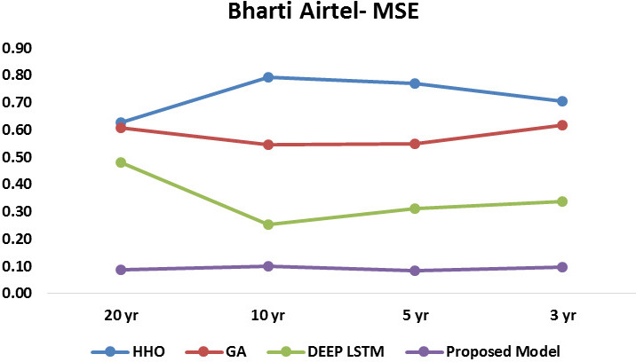
RMSE of Asian Paints.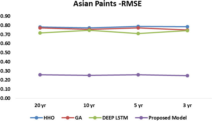

Table 5

RMSE results of Bajaj Auto

Stock	Historical data duration (in years)	Metric	HHO	GA	Deep LSTM	Proposed model IRRLSTM
Bajaj Auto	20	RMSE	0.776	0.761	0.739	0.250
Bajaj Auto	10	RMSE	0.763	0.760	0.754	0.250
Bajaj Auto	5	RMSE	0.763	0.763	0.752	0.246
Bajaj Auto	3	RMSE	0.765	0.757	0.755	0.248

Table 6

RMSE results of Bharti Airtel

Stock	Historical data duration (in years)	Metric	HHO	GA	Deep LSTM	Proposed model IRRLSTM
Bharti Airtel	20	RMSE	0.792	0.779	0.692	0.297
Bharti Airtel	10	RMSE	0.890	0.890	0.502	0.316
Bharti Airtel	5	RMSE	0.878	0.741	0.557	0.290
Bharti Airtel	3	RMSE	0.839	0.786	0.581	0.311

Figure 8.

RMSE of Bajaj Auto.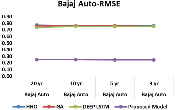

Figure 9.

RMSE of Bharti Airtel.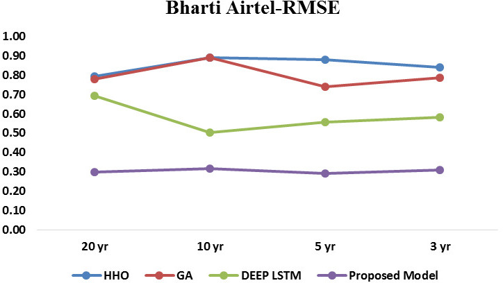

Figure 10.

MSE of deep LSTM vs proposed recurrent rider LSTM.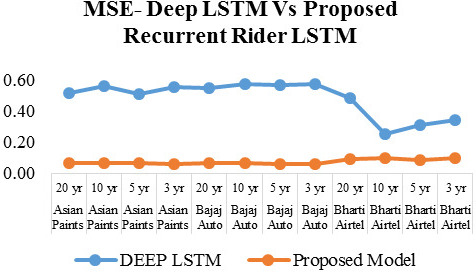

Figure 11.

RMSE of deep LSTM vs proposed recurrent rider LSTM.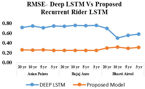

4.2 Comparative analysis

In this subsection, three datasets are used to compare the proposed Deep Recurrent Rider LSTM with existing approaches in terms of the assessment criteria.

The analysis of developed model with respect to MSE is presented in Fig. 4. When the delay is 5000, the MSE achieved by developed improved Recurrent Rider LSTM is 0.067, 0.063 and 0.088 for the three twenty year time series dataset of Asian Paints, Bajaj Auto, and Bharati Airtel respectively. Similarly for the ten, five and three year time series dataset of stocks as shown in Figs 4–6, it obtained MSE of 0.064, 0.063, 0.100 and 0.066, 0.061, 0.084 and 0.062, 0.061, 0.097 respectively. The analysis of results of MSE conclude that the more time series data is helpful in reducing the error rate.

Figure 12.

Empirical MSE results.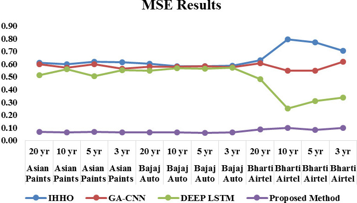

Figure 13.

Empirical RMSE results.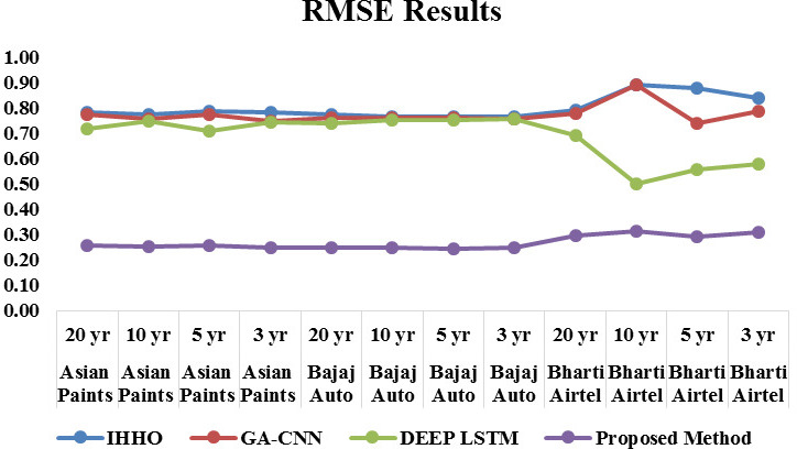

Table 7

Existing methods and proposed method results

Stock	Historical data duration (in years)	Metric	HHO	GA	Deep LSTM	Proposed method
Asian Paints	20 yr	MSE	0.611368	0.59822	0.513617	0.066839
Asian Paints	20 yr	RMSE	0.7819	0.773447	0.716671	0.258532
Asian Paints	10 yr	MSE	0.596693	0.572478	0.558691	0.063867
Asian Paints	10 yr	RMSE	0.772459	0.756623	0.747457	0.25272
Asian Paints	5 yr	MSE	0.619063	0.598277	0.504399	0.066373
Asian Paints	5 yr	RMSE	0.786806	0.773483	0.710211	0.257629
Asian Paints	3 yr	MSE	0.614188	0.562581	0.549979	0.06163
Asian Paints	3 yr	RMSE	0.783702	0.750054	0.741606	0.248255
Bajaj Auto	20 yr	MSE	0.602096	0.579374	0.545784	0.062653
Bajaj Auto	20 yr	RMSE	0.775949	0.761166	0.738772	0.250306
Bajaj Auto	10 yr	MSE	0.58277	0.577363	0.56843	0.062599
Bajaj Auto	10 yr	RMSE	0.763394	0.759844	0.753943	0.250198
Bajaj Auto	5 yr	MSE	0.582467	0.581417	0.564819	0.06054
Bajaj Auto	5 yr	RMSE	0.763196	0.762507	0.751544	0.246049
Bajaj Auto	3 yr	MSE	0.585151	0.573078	0.570448	0.061389
Bajaj Auto	3 yr	RMSE	0.764952	0.757019	0.75528	0.247768
Bharti Airtel	20 yr	MSE	0.627711	0.606925	0.479377	0.088393
Bharti Airtel	20 yr	RMSE	0.792282	0.779054	0.69237	0.29731
Bharti Airtel	10 yr	MSE	0.792838	0.545921	0.251846	0.099751
Bharti Airtel	10 yr	RMSE	0.890414	0.890414	0.501842	0.315834
Bharti Airtel	5 yr	MSE	0.77136	0.549286	0.310175	0.084138
Bharti Airtel	5 yr	RMSE	0.878271	0.741138	0.556934	0.290065
Bharti Airtel	3 yr	MSE	0.704275	0.617236	0.337118	0.096785
Bharti Airtel	3 yr	RMSE	0.839211	0.785644	0.580618	0.311103

Table 8

D’Agostino-Pearson test (significance level of 0.05)

Dataset method	Statistic	$p$ -value	Result
IHHO	5.36179	0.0685	H0 is accepted
GA	3.62947	0.16288	H0 is accepted
Deep LSTM	0.67654	0.713	H0 is accepted
Proposed method	2.51181	0.28482	H0 is accepted

Figure 14.

Existing methods versus proposed method.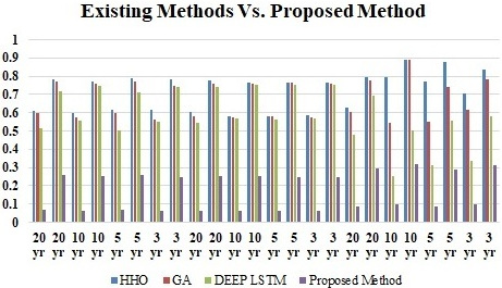

Similarly the analysis of developed model with respect to RMSE is depicted in Fig. 4. When the delay is 5000, the RMSE achieved by developed improved Recurrent Rider LSTM is 0.259, 0.250, and 0.297 for the three twenty year time series dataset of Asian Paints, Bajaj Auto, and Bharati Airtel respectively. Similarly for the ten, five and three year time series dataset of stocks as shown in Figs 7–9, model obtained RMSE of 0.253, 0.250, 0.316 and 0.258, 0.246, 0.290 and 0.248, 0.248, 0.311 respectively. Here also observation of results of RMSE depict that the large time series data is providing reduce error rate. Figure 14 shows the collective comparison of MSE and RMSE result of existing methods such as HHO, Genetic algorithm and Deep LSTM with proposed method of improved Deep LSTM. Results clearly indicates the effectiveness of proposed method which shows lowest error rate for the model. Cross verification of results are performed to ensure effectiveness and not to get stuck into local maxima with various sectors stock dataset. Proposed method is outperforming for different sector stock which shows efficiency of model for all kind of dataset of stocks. Time efficiency method is proportional to the number of technical indicators as a parameter and validation iteration performed. Proposed method select features on the basis of their importance hence it has less time complexity.

Study and results of normal deep LSTM and proposed improved recurrent rider long short term memory model from Figs 10 and 11 proposed LSTM outperforms in terms of MSE & RMSE. Here no kind of optimization training is provided to the proposed RNN LSTM model. Further scope of study and experiment of optimization approaches is to be studied.

5. Conclusion and future work

The price of stocks fluctuates over time on the stock market. In reality, along with its non-linearity, dynamic nature, and complexity, stock market prediction continues to be a significant challenge. The researchers’ primary focus in the previously published publications was empirical methods. Financial time series data is not a typical use for deep learning. The deep learning model, which also has the capabilities to accommodate the time-series data well, is used in this analysis. In this paper, an effective stock market prediction method with reduced error rate called improved Recurrent Rider LSTM is suggested. Proposed LSTM model seems to be effective for performed conditions due to its rider approach and effective feature selection approach. It also focus on importance of technical indicators as a feature for proposed model. Study and analysis of the results in the research depict the effectiveness of LSTM in processing the time series data. Overall evaluation metric results observed that proposed LSTM proved to be outperforming as compare to earlier methods such as deep LSTM, HHM & GA method. Here LSTM operates without the aid of an optimization training method to best suit the answer, but future research may examine LSTM performance in conjunction with more complex optimization techniques.

References

Bouktif

Fiaz

Awad

. Augmented Textual Features-Based Stock Market Prediction. IEEE Access. 2020; 8: 40269-40282. 9016182. doi: 10.1109/ACCESS.2020.2976725.

Liu

Long

. An improved deep learning model for predicting stock market price time series. Digital Signal Processing. 2020; 102: 1051-2004. doi: 10.1016/j.dsp.2020.102741.

, et al. An Improved Harris’s Hawks Optimization for SAR Target Recognition and Stock Market Index Prediction. IEEE Access. 2020; 8: 65891-65910.

Chung

Shin

. Genetic algorithm-optimized multi-channel convolutional neural network for stock market prediction. Neural Comput & Applic. 2020; 32: 7897-7914. doi: 10.1007/s00521-019-04236-3.

Nabipour

Nayyeri

Jabani

, et al. Deep learning for Stock Market Prediction. Entropy. 2020; 22: 840.

Khan

Ghazanfar

Azam

, et al. Stock market prediction using machine learning classifiers and social media, news. J Ambient Intell Human Comput. 2022; 13: 3433-3456. doi: 10.1007/s12652-020-01839-w.

Pang

Zhou

Wang

, et al. An innovative neural network approach for stock market prediction. J Supercomput. 2020; 76: 2098-2118. doi: 10.1007/s11227-017-2228-y.

Ananthi

Vijayakumar

. Retraction Note to: Stock market analysis using candlestick regression and market trend prediction (CKRM). J Ambient Intell Human Comput. 2022. doi: 10.1007/s12652-022-04067-6.

Kohavi

John

. Wrappers for feature subset selection. Artificial Intelligence. 1997; 97: 273-324. doi: 10.1016/S0004-3702(97)00043-X.

10.

Binu

Kariyappa

. Rider Deep LSTM Network for Hybrid Distance Score-based Fault Prediction in Analog Circuits. IEEE Transactions on Industrial Electronics. 2020. doi: 10.1109/TIE.2020.3028796.

11.

Inoue

Nishida

. Deep recurrent neural network for mobile human activity recognition with high throughput. Artif Life Robotics. 2018; 23: 173-185. doi: 10.1007/s10015-017-0422-x.

12.

Askarzadeh

. A novel metaheuristic method for solving constrained engineering optimization problems: Crow search algorithm. Computers & Structures. 2016; 169: 1-12. doi: 10.1016/j.compstruc.2016.03.001.

13.

Kaveh

Zaerreza

. Shuffled shepherd optimization method: a new Meta-heuristic algorithm. Engineering Computations. 2020; 7: 2357-89. doi: 10.1108/EC-10-2019-0481.

14.

Stock Dataset. Available from: http://www.moneycontrol.com/stocks/histstock.php?ex=N&sc_id=AMF&mycomp=Apple%20Mutual%20Fund. Accessed on March, 2021.

15.

Attigeri

Manohara Pai

Pai

Nayak

. Stock market prediction: A big data approach. In: TENCON 2015 – 2015 IEEE Region 10 Conference. Vol. 2016-January. Institute of Electrical and Electronics Engineers Inc; 2016. pp. 7373006. doi: 10.1109/TENCON.2015.7373006.

16.

Bollen

Mao

Zeng

. Twitter mood predicts the stock market. Journal of Computational Science. 2011 Mar 1; 2(1): 1-8.

17.

Porshnev

Redkin

Shevchenko

. Machine Learning in Prediction of Stock Market Indicators Based on Historical Data and Data from Twitter Sentiment Analysis. In: IEEE 13th International Conference on Data Mining Workshops. Dallas; 2013. pp. 440-444. doi: 10.1109/ICDMW.2013.111.

18.

Schöneburg

. Stock price prediction using neural networks: A project report. Neurocomputing. 1990; 2: 17-27.

19.

Tambi

. Forecasting Exchange Rate: A Univariate Out-of-Sample Approach (Box-Jenkins Methodology). The IUP Journal of Bank Management. IV. 2005; pp. 60-74.

20.

Brock

, et al. Simple Technical Trading Rules and the Stochastic Properties of Stock Returns. The Journal of Finance JSTOR. 1992; 47(5): 1731-64. doi: 10.2307/2328994.

21.

Hansen

McDonald

, et al. Time Series Prediction with Genetic-Algorithm Designed Neural Networks: An Empirical Comparison with Modern Statistical Models. Computational Intelligence. 1999; 15: 171-184. doi: 10.1111/0824-7935.00090.

22.

Thangavel

Kumar

. Optimization of code book in vector quantization. Ann Oper Res. 2006; 143: 317-325. doi: 10.1007/s10479-006-7391-0.

23.

Thangavel

Kumar

Aranganayagi

. Pattern Clustering Neural Networks. In: Proceeding of International Conference on Vision 2020: The Strategic Role of Operations Research. Allied Publishers; 2005. pp. 662-681.

24.

Khashei

Bijari

. An artificial neural network (p, d, q) model for timeseries forecasting. Expert Syst Appl. 2010; 37: 479-489. doi: 10.1016/j.eswa.2009.05.044.

25.

Refenes

Zapranis

Francis

. Stock performance modeling using neural networks: a comparative study with regression models. Neural Networks. 1994; 7(2): 375-388. doi: 10.1016/0893-6080(94)90030-2.

26.

Martinez

da Hora

de M Palotti

, et al. From an artificial neural network to a stock market day-trading system: A case study on the BM&F BOVESPA. In: 2009 International Joint Conference on Neural Networks. IEEE; 2009. pp. 2006-2013.

27.

Mettenheim

Breitner

. Forecasting daily highs and lows of liquid assets with neural networks. Leibnitz: Springer; 2012. pp. 253-258.

28.

Adebiyi

Adewumi

Ayo

. Comparison of ARIMA and Artificial Neural Networks Models for Stock Price Prediction. Journal of Applied Mathematics. 2014. doi: 10.1155/2014/614342.

29.

Chen

Zhou

Dai

. A LSTM-based method for stock returns prediction: A case study of China stock market. In: Luo

Ogan

Zaki

Haas

Ooi

Kumar

Rachuri

Pyne

Hsiao

MH-I

, editors. Proceedings – 2015 IEEE International Conference on Big Data, IEEE Big Data 2015. Institute of Electrical and Electronics Engineers Inc.; 2015. pp. 2823-2824. 7364089. doi: 10.1109/BigData.2015.7364089.

30.

Qiu

. Predicting the Direction of Stock Market Index Movement Using an Optimized Artificial Neural Network Model. PloS one. 2016; 11(5): e0155133. doi: 10.1371/journal.pone.0155133.

31.

Long

, et al. An integrated framework of deep learning and knowledge graph for prediction of stock price trend: An application in Chinese stock exchange market. Appl Soft Comput. 2020; 91: 106205.

32.

Rekha

Sravanthi

Somula

Govinda

. Prediction of Stock Market Using Neural Network Strategies. Journal of Computational and Theoretical Nanoscience. 2019; 16(5): 2333-2336. doi: 10.1166/jctn.2019.7895.

33.

Pang

Zhou

Wang

Lin

Chang

. An innovative neural network approach for stock market prediction. Journal of Supercomputing. 2018 Jan 12. doi: 10.1007/s11227-017-2228-y.

34.

Suman

Parasar

Rathod

. Seeded region growing segmentation on ultrasound image using particle swarm optimization. In: IEEE International Conference on Computational Intelligence and Computing Research (ICCIC). 2015. pp. 1-6. doi: 10.1109/ICCIC.2015.7435715.

35.

d’Agostino

Pearson

. Tests for departure from normality. Empirical results for the distributions of b2 and b1. Biometrika. 1973; 60(3): 613-622. doi: 10.1093/biomet/60.3.613.

36.

Patil

Parasar

Charhate

. A Literature Review on Machine Learning Techniques and Strategies Applied to Stock Market Price Prediction. Emerging Trends in Data Driven Computing and Communications. 2021; 121-35. doi: 10.1007/.

37.

Patil

Parasar

Charhate

. Wrapper based feature selection and optimization enabled hybrid deep learning framework for stock market prediction. International Journal of Information Technology & Decision Making. doi: 10.1142/S0219622023500116.

An effective deep learning model with reduced error rate for accurate forecast of stock market direction

Abstract

Keywords

1. Introduction

2. Literature review

2.1 Approaches

2.2 Challenges

3. Proposed method

3.2 Data preprocessing

3.3 Feature extraction

3.3.1 Average true range (ATR)

3.3.2 Rate of change (ROC)

3.3.3 Relative strength index (RSI)

3.3.4 Average directional movement index (ADMI)

3.3.5 William’s % R

3.3.6 Money flow index (MFI)

3.3.7 Triple exponential average (TRIX)

3.4 Feature selection

3.5 Data augmentation

3.6 Cross validation

3.7.1 Rider Deep LSTM network

3.7.2 Deep RNN

4. Results and discussion

Table 1 MSE results of Asian Paints

Table 3 MSE results of Bharti Airtel

References

Table 1
MSE results of Asian Paints

Table 3
MSE results of Bharti Airtel