
Abstract
Background:
Alzheimer’s disease (AD) is a progressive neurodegenerative disease that results in cognitive decline, dementia, and eventually death. Diagnosing early signs of AD can help clinicians to improve the quality of life.
Objective:
We developed a non-invasive approach to help neurologists and clinicians to distinguish probable AD patients and healthy controls (HC).
Methods:
The patients’ gaze points were followed based on the words they used to describe the Cookie Theft (CT) picture description task. We hypothesized that the timing of words enunciation aligns with the participant’s eye movements. The moments that each word was spoken were then aligned with specific regions of the image. We then applied machine learning algorithms to classify probable AD and HC. We randomly selected 60 participants (30 AD and 30 HC) from the Dementia Bank (Pitt Corpus).
Results:
Five main classifiers were applied to different features extracted from the recorded audio and participants’ transcripts (AD and HC). Support vector machine and logistic regression had the highest accuracy (up to 80% and 78.33%, respectively) in three different experiments.
Conclusions:
In conclusion, point-of-gaze can be applied as a non-invasive and less expensive approach compared to other available methods (e.g., eye tracker devices) for early-stage AD diagnosis.
Keywords
INTRODUCTION
According to [1], approximately 6.2 million Americans aged 65 and older will be living with Alzheimer’s disease (AD) by 2023. This number will increase to 12.7 by 2050. According to research findings, more than 747,000 Canadians suffer from AD or other forms of dementia [2]. Increasing numbers of people with AD have attracted the attention of many scientists looking for early signs of the disease. In recent years, AD has become an increasingly interesting and important topic inscience.
AD is a degenerative disease that progresses with time. AD initial symptoms can appear 20 years before the onset of symptoms [3]. Consequently, there is considerable interest among scientists in detecting early signs of AD [4–6]. For detection, doctors and clinicians are using various cognitive tests. The picture description task is one of those tests [7].
Along the same line, many clinical pieces of research show that AD affects eye movement in people with AD [4]. Eye movement analysis seems to be a valuable method for detecting early signs of AD [8].
Medical studies have shown that eye movement disorders can be related to various neurological diseases. Eye movement characteristics have been used as biomarkers of Parkinson’s disease, AD, schizophrenia, and other diseases. However, due to the unknown medical mechanism of some diseases, it is challenging to establish an intuitive correspondence between eye movement characteristics and diseases [4].
Studies have shown that AD causes visual deficits, including reduced ability to detect motion, loss of depth perception, decreased peripheral vision, and difficulty recognizing colors [9]. Identifying these deficits led researchers to investigate eye movements and fixations as biomarkers of AD. Indeed, according to recent research, eyes (including eye movements) may reveal early signs of AD and offer a convenient window into the disease’s progression [10–12].
Zhengyan et al. [13] (2022) evaluated a deep learning model incorporating speech and eye-tracking to predict dementia with three categories: mild cognitive impairment (MCI), AD, and healthy controls (HC). Automatic speech recognition (ASR) and regional picture recognition (RPR) were applied for data pre-processing. They classified patients with dementia and HC with 84.26% accuracy.
Franceschiello et al. [14] (2022) proposed an approach with machine learning and neural network techniques to analyze saccadic eye movement trajectories. They achieved up to 86% accuracy.
Barral et al. [5] presented a non-invasive approach for classifying the AD and HC participants based on speech and eye movement analysis. Tobi Pro Studio software was utilized as an eye tracker tool to extract the required features for classification. They evaluated three classification algorithms: logistic regression (LR), random forest (RF), and Gaussian Naive Bayes (GNB). They had 73% accuracy. With a combination of eye-tracking and speech analysis, the accuracy of the classification improved to 80%.
Fraser et al. [15] evaluated a machine learning model applied for eye-tracking data to detect MCI (27 MCI and 30 HC subjects). Their experiment was on reading aloud versus silently. They applied three classification algorithms: Naive Bayes (NB), support vector machine (SVM), and logistic regression (LR). They achieved up to 86% accuracy. Biondi et al. [16] reformed an experiment using a deep-learning approach to distinguish between the behavior of people with AD compared to HC from reading. They used an eye tracker tool to differentiate between eye-movement the behavior of people with AD versus HC (26 AD and 43 HC). They used the trained auto-encoders and soft-max to build a deep neural network, which allowed them to identify AD patients with 90.78% accuracy.
Lagun et al. [17] used the Visual Paired Comparison task as a recognition memory test that can help to detect the memory impairments associated with MCI. Participants contained (10 MCI, 20 AD, and 30 HC). They reported 87% accuracy using an SVM classifier. In addition, Mirheidari et al. [6] proposed a non-invasive method for capturing identical visual features for AD and HC people describing the Cookie Theft (CT) picture with their speech. The data was taken from the Dementia Bank and included 89 HC and 168 AD subjects. They used an ASR to align words with regions. They achieved 80% F1-score using the LR classifier.
Eye movement information plays an essential role in detecting AD. Medical findings show that people with AD have different eye-movement patterns compared to HC. However, using a patient’s eye movement for diagnosing at early steps of AD is challenging. Therefore, we propose a novel method to support diagnosis, classifying AD at early steps using words. We analyze Pitt Corpus [18, 19] transcripts and audios, considering the gaze points inferred from the enunciation of words from probable AD patients compared to HC.
MATERIALS AND METHODS
This section describes the data used and the required pre-processing steps. Five different classification approaches are applied and compared in terms of accuracy. Figure 1 shows the methodology steps to classify the AD and HC participants.

Steps to classify AD and HC individuals, based on extracted features from audios and transcripts of the CT picture.
Data description: CT and Pitt Corpus
In pathology studies, the Boston picture description task is mostly used in clinical neurology tests to detect cognitive impairment and patients with early dementia or AD [7]. In this work, we focused on the CT image, which is part of the above-mentioned task.
For any picture description task, the interviewer asks the participants to describe an image (CT image, Fig. 2). The participants are asked to look at the image and describe the following scene. It is common for AD patients to mention less salient details such as the plants and trees in the garden or the clothes worn by the characters, or the items of crockery beside the sink. Patients with no neurological impairment express these details at the end of their descriptions, after the most salient information has already been conveyed, acknowledging the reduced importance of these details [7].
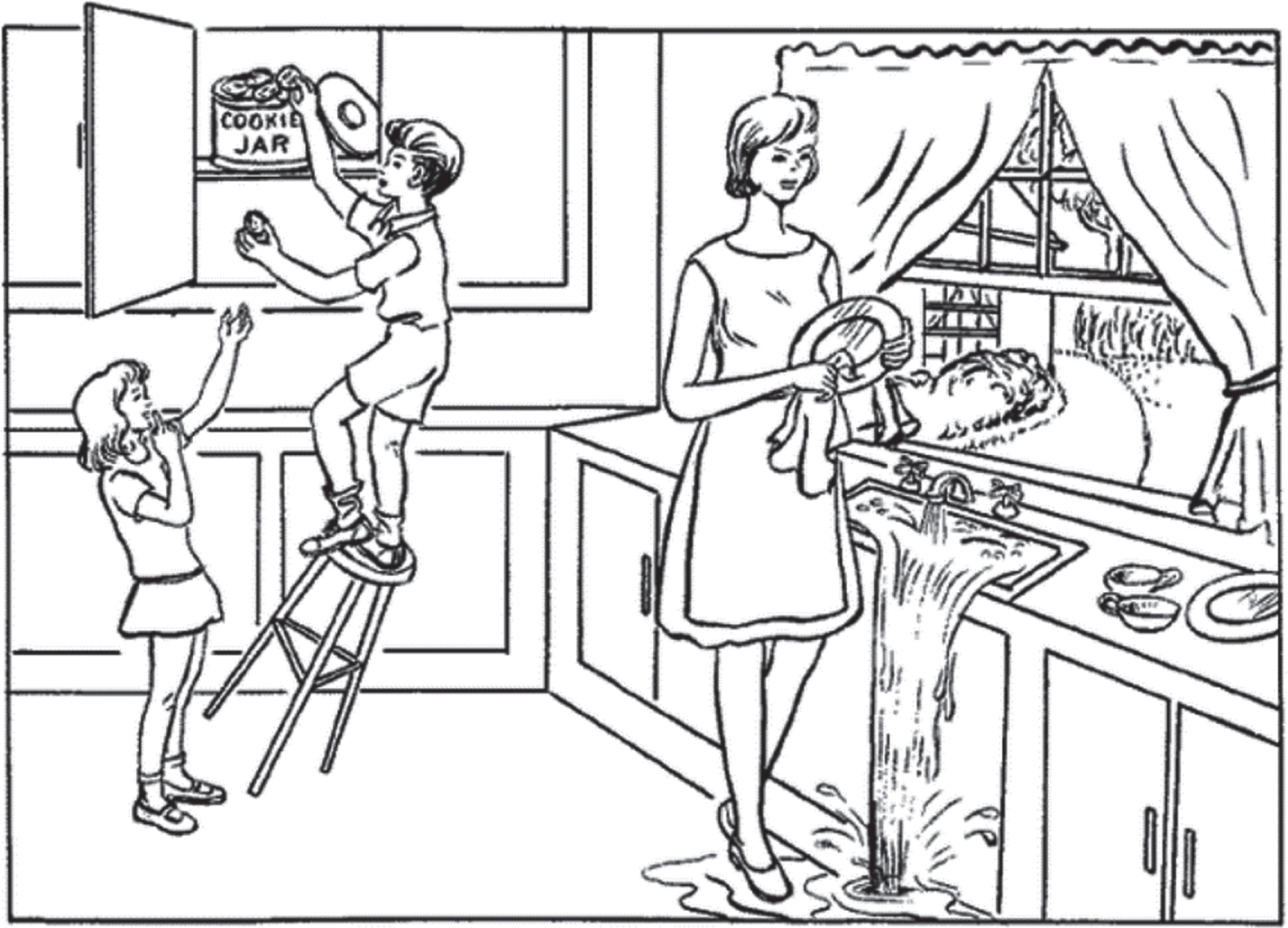
Cookie Theft picture description from the Boston Diagnostic Aphasia Examination. Taken from Kaplan et al. (2001).
Our data consists of the Pitt Corpus transcripts and audios from the Dementia bank [18, 19]. In this data set, the CT picture was given to different groups of participants for a study at the University of Pittsburgh School of Medicine. The participants for the test included neurotypical older adults, people with probable AD, MCI, and other people with dementia diagnoses. This data set contains 517 transcriptions (257 probable AD, 217 HC, and 43 MCI). We randomly selected 30 HC participants and 30 probable AD participants, including the recorded audio and text descriptions of the CT image.
HC included 20 women (F) and 10 men (M), while probable AD participants included 18 women and 12 men. The mean age for AD was 70.72, and the mean year of education was 12.53 years. These numbers for HC were 68 and 14.46, respectively. Table 1 shows demographic information for participants with AD and HC. Figure 2 shows the CT picture description task.
Demographic information for 30 participants with probable Alzheimer’s disease (AD) and 30 healthy controls (HC)
Age, sex, and education are given in the format: ([mean]±[standard deviation]).
Data pre-processing using Praat Software
Working with transcripts carries multiple challenges. Transcripts may appear in a different format, such as plain text files or transcription files (.cha). We used the Praat [20] tool to extract the information, which are words that refer to a specific region in the CT picture with time spent for each region. A region is a particular subject/object in the image (e.g., the woman, the sink).
We divided the audio into two layers to associate the transcripts and audio with the picture. The first layer segments the audio based on words (our keywords) within transcripts. The second layer reproduces the same segments but uses regions to annotate them. For example, in Fig. 3, layer 1 presents the words “woman let the water fall floor.” This segment is associated with region 2 in the second layer. Time stamps of regions are then used to infer the eye movements of the patient. We will use the abbreviation DEM (Deduced Eye Movements) to refer to these associations.
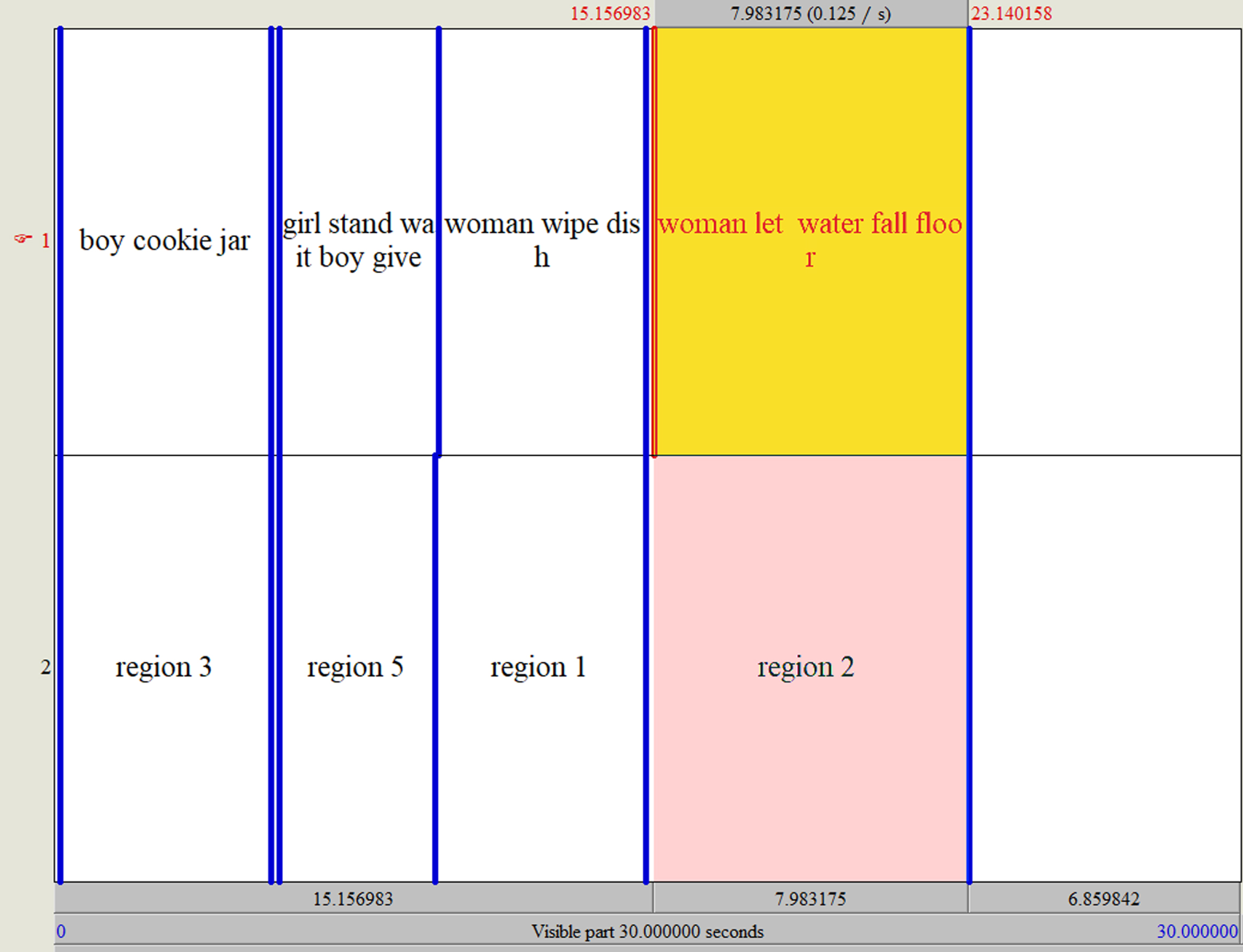
Praat is a free package for speech analysis in phonetics and gives the ability to segment different intervals.
To classify AD and HC, we investigated different patterns for HC and AD considering the differences between these groups in their DEM. As we listened to the audio, we manually entered information into the Praat software, segmenting each part according to the region. For example, we listened to the first participant’s audio file.
If that person talked about a specific noun or action related to the regions on our picture, we took it as one segment. Then with the help of a transcript of that conversation, we corresponded each word and action to the same audio section and related region. We applied the same method to all participants.
Praat software provides the time duration for each segmentation as a text grid file. The extracted information from the text grid file includes starting time (xmin), ending time (xmax), text (the related content of the transcript), and region. Figure 4 show an example of a text grid file.
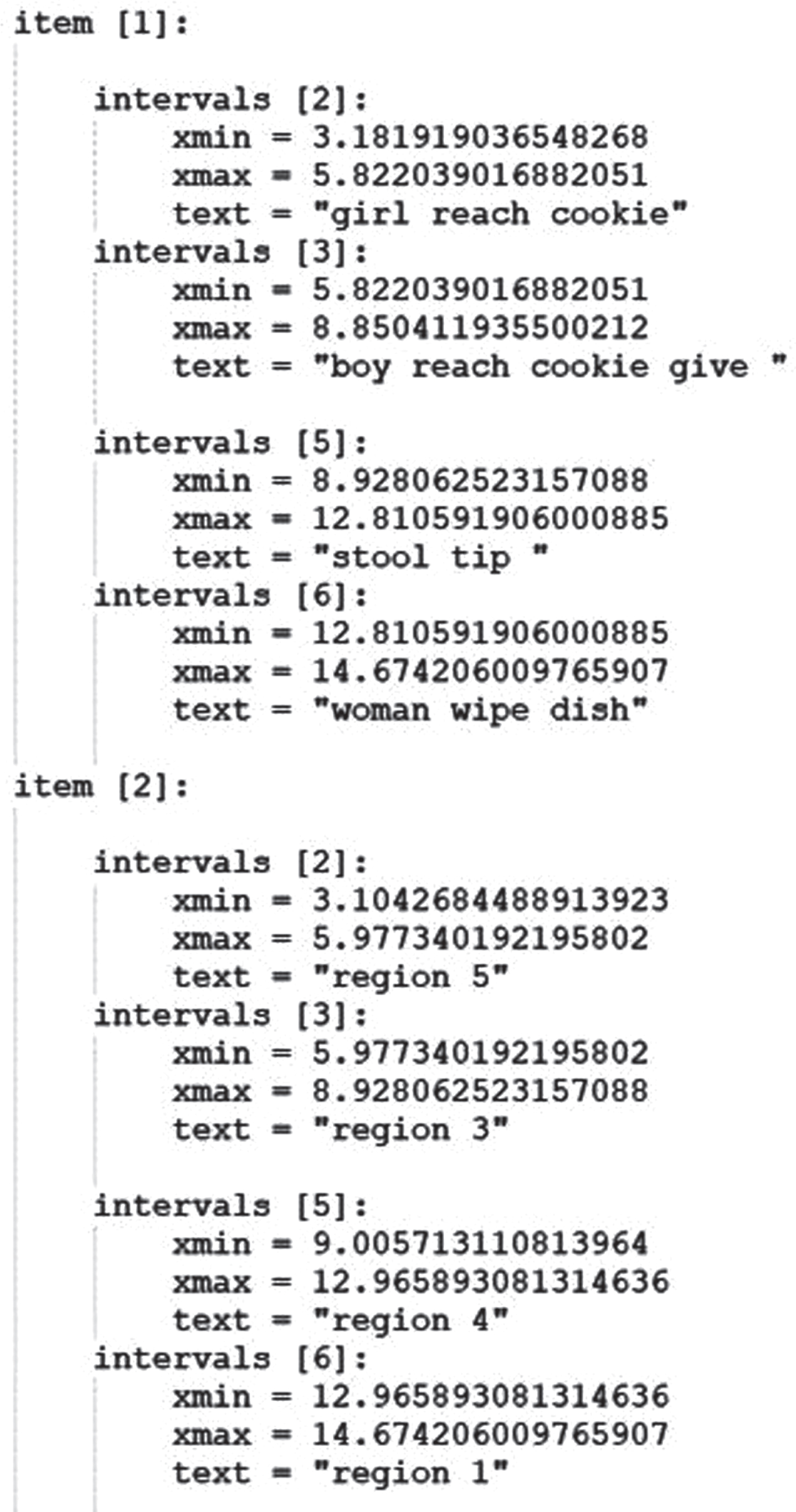
Text grid file corresponding region and words with time.
As it is shown in Fig. 4, the text grid file contains two sections (item 1 and item 2). Item 1 represents words and sentences with start and end times. Item 2 represents the region with the start and end point, in which two sections are connected to each other. Start and end time for each keyword associated with a specific region.
The time which is xmin and xmax are approximately the same in both the words section (item 1) and region section (item 2). For instance, in item 1, interval 2 xmin and xmax are equal with interval 2 in item 2.
Feature extraction
Different feature extraction approaches were applied to classify the AD and HC participants with the best accuracy.
Feature extraction based on words and audios
The extracted information from Praat software includes xmin and xmax, which are the start and finish times of a word or sentence used to explain a region defined in the CT picture. Figure 5 shows an example of our information extraction from the data of one of the participants.
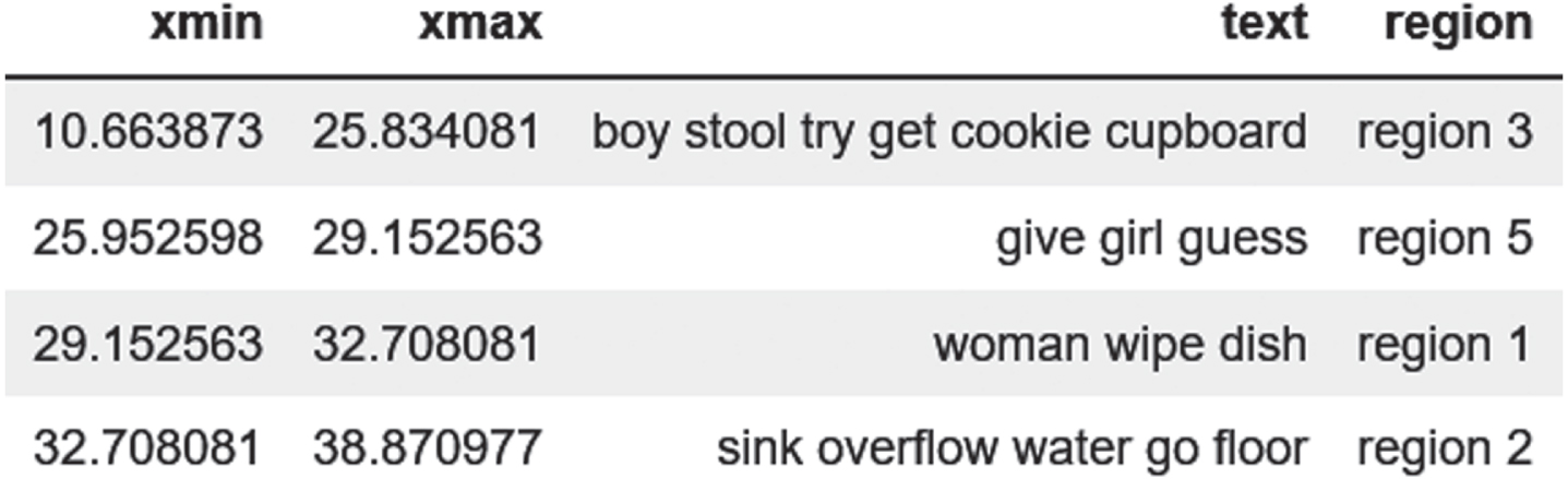
The information extracted from our audios and transcripts with Praat software (The time that shows in the picture is based on seconds).
Region defining and word alignment on the picture
We divided the CT image into different regions and associated each region with the key nouns and verbs extracted from the transcripts.
For instance, all mentioned words that have a similar meaning, such as “brother,” “boy,” “kid,” theft, and cookie, are associated with “region 3”. Figure 6 shows how we associate specific words and sentences to particular regions.
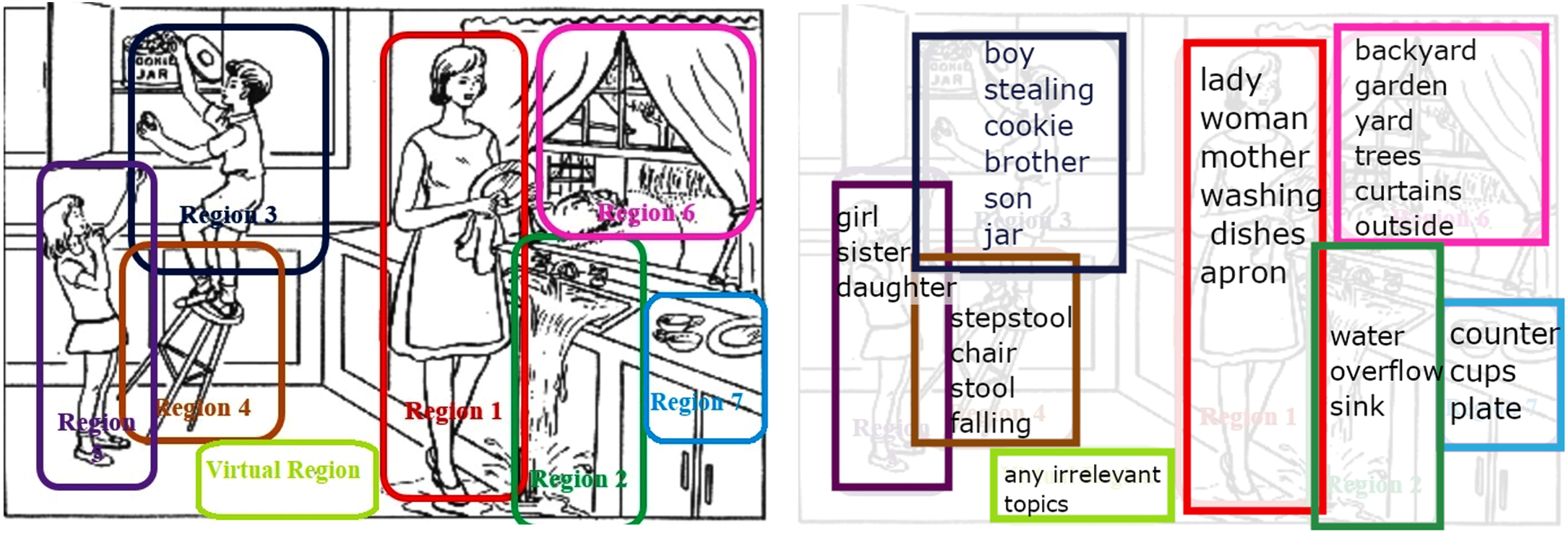
Words from transcript associated with regions in CT image.
By analyzing the recorded audio and transcripts of the picture description task, noticeable differences between the AD and HC participants were observed. Mainly these differences were detected in the time spent describing a specific region or the entire time spent on the picture description. AD patients typically spend more time. AD people spent more time describing the image partly because their discourse was filled with silences and pauses.
Moreover, the number of regions of interest mentioned by AD participants was different compared to the HC participants. AD individuls showed less interest in discussing the whole picture and mentioning all regions. In contrast, HC individuals were very detail-oriented and mentioned most regions. Some specific regions in the image were pointed out by AD participants frequently (e.g., the boy) or almost ignored by them completely (e.g., details in the backyard).
In some cases, AD participants mentioned objects or characters that did not exist in the CT picture. These objects and characters were considered to belong to a virtual region. As mentioned above, when AD people talked about the picture’s virtual region, they seemed distracted. The picture in itself is probably reminding them of their childhood memories. For instance, one patient was singing a childhood song. Another was talking about a “father” even though no man exists in the picture. These signs of distractions gave the impression that the patients might have imagined some characters that do not exist in the CT picture.
Visualizing scan paths of CT from transcript
Using the extracted text grid file from Praat, we followed the participants’ DEM on the picture and found the area and regions of interest. Then we compared the AD and HC participants’ regions of interest and analyzed the specific words used by each group.
Listening to the audio and analyzing the transcripts, we found out HC individuals’ gaze fixation on different areas (regions) is more sequenced and arranged. Figure 7 shows the scan path of an HC and AD participants. The HC participant started by describing one region and then moved to the closest regions, which means that their eye movement is very organized. But for AD patients, the regions’ descriptions are disorganized and not sequenced. This phenomenon is amplified by the fact that some patients are distracted and talk about virtual regions’ irrelevant subjects not included in the picture. For example, the AD patient in Fig. 7 talks about the boy (1), then about something that is not in the picture; then he talks about the woman (2) and again about something that is not relevant (3), then about the stool (4).
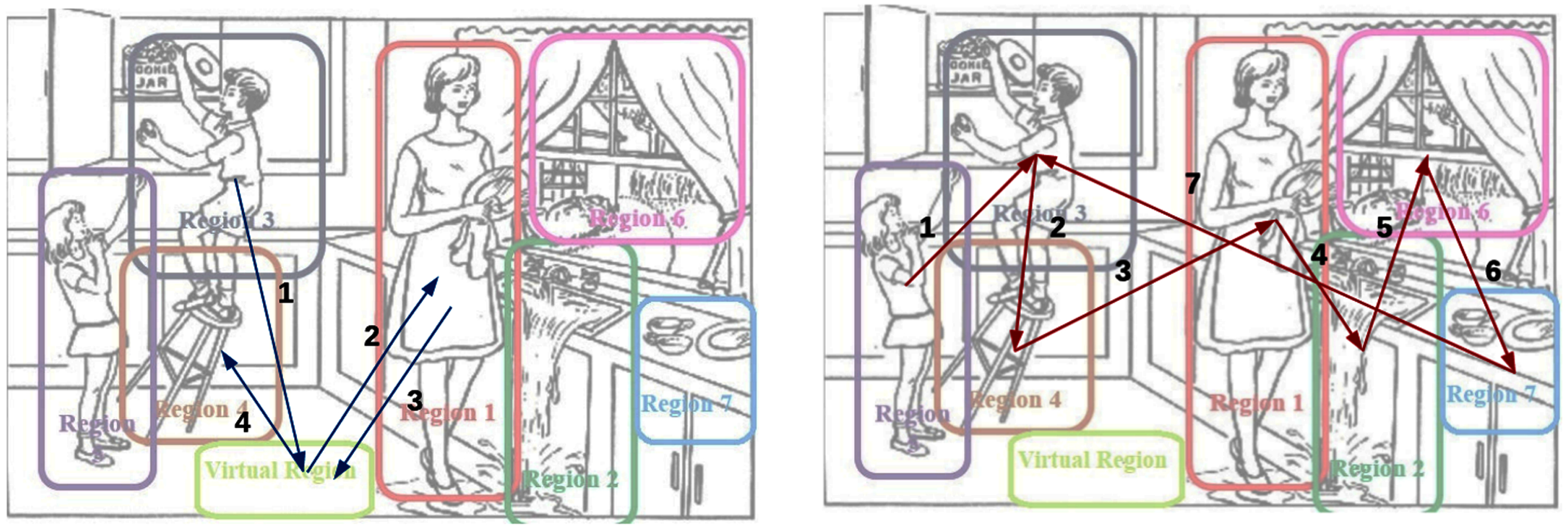
Scan path of the AD patient (left) versus HC individual (right).
Feature extraction based on trajectory
A trajectory analysis aims to characterize participants’ behavior, capturing the scan path pattern. Different methods exist to generate trajectory features. Following [21], we chose the geometric distance method.
A trajectory is a path that connects sequentially the centers of each visited region during the description of the CT image. Figure 8 shows a trajectory during the CT. As it shows, we have four different visited regions in a sequence (this trajectory corresponds to one of our AD participants).
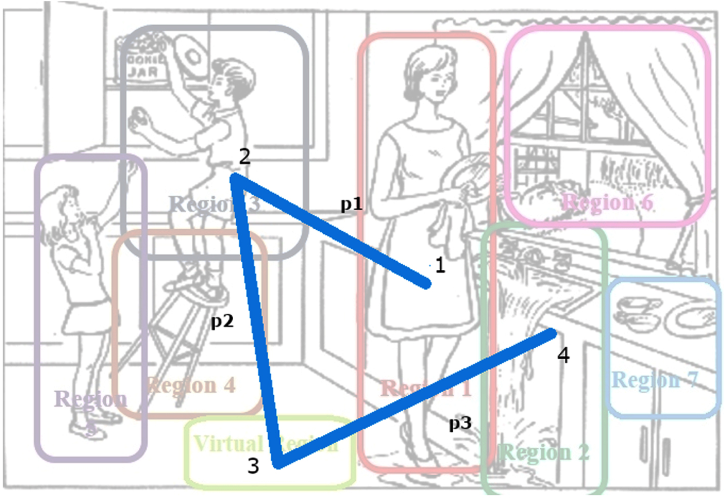
An example of a patient’s trajectory during the CT picture description. P1, P2, and P3 are the distances between points (1,2,3,4).
The geometric distance (in pixel) method extracts features by segmenting the path in multiple resolutions. Figure 9 shows how we extract the first feature with the geometric distance method.
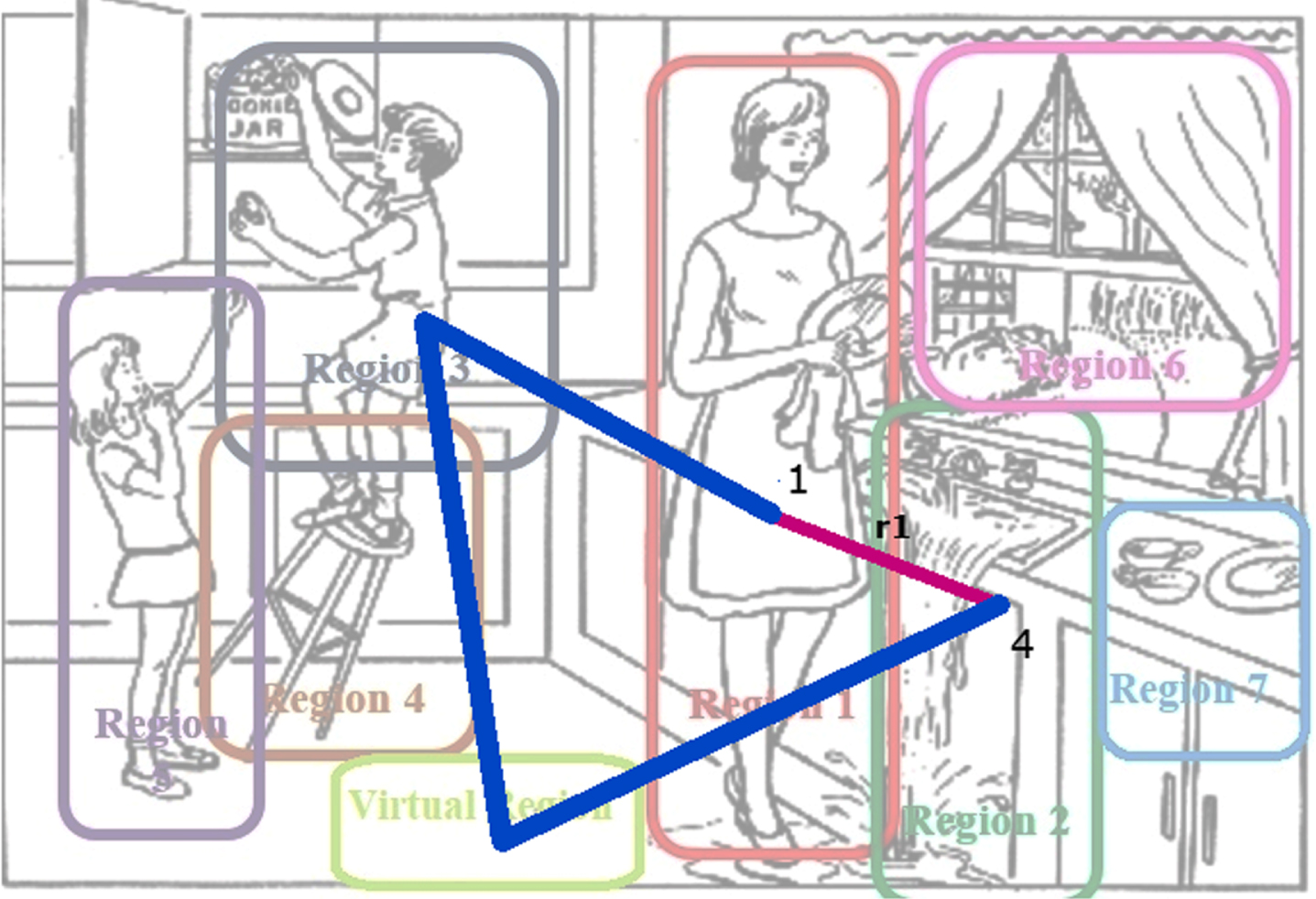
Extract first feature with geometric distance method from point 1 to point 4. r1 is the first feature.
In the first feature extraction, we calculate the length of the entire trajectory (P) and the distance between the starting and ending points (r1, point 1, and point 4, respectively). f1 is the first feature.
For extracting the following two features (f2 and f3), we considered the middle point (m) of the entire trajectory from point 1 to point 4; r2, r3 are the distances from the start point (1) to (m) and from (m) to the endpoint (4) (Fig. 10).
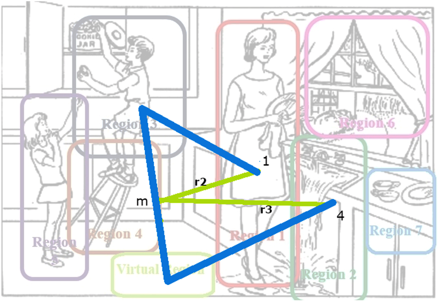
Extract two features with geometric distance method from point 1 to 4. m is a parameter that shows the division of the whole trajectory. r2 and r3 are distance from 1 to m and m to point 4.
For extracting the following three features (f4, f5 and f6), we divided the entire trajectory into two points (n&d) from point 1 to point 4; (r4, r5, r6), are the distances from the start point (1) to (n) from (n) to (d) and from (d) to endpoint (4) the endpoint (4) (Fig. 11).
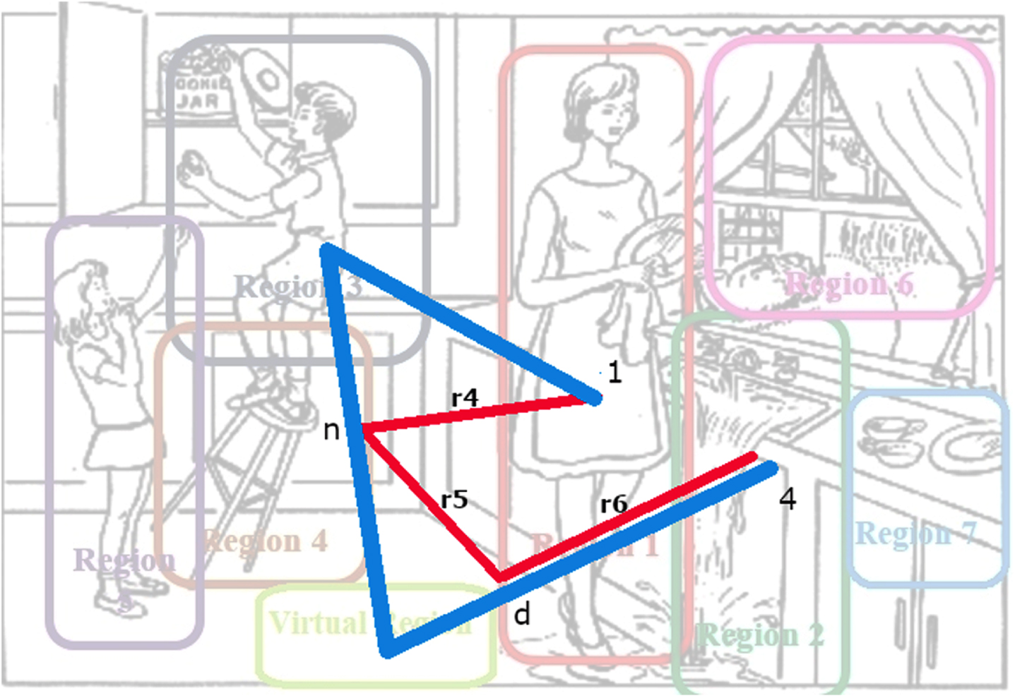
Extract next three features with geometric distance method from point 1 to point 4. n and d are division points of the whole trajectory. r4, r5, r6 are distances from point 1 to n, point n to point d and from point d$ to point 4 respectively.
Additionally, we applied the trajectory method by increasing the resolution (number of points in a specific trajectory). Hence, we extracted a higher number of features and feature vectors for AD and HC classification.
The feature vectors for both groups were extracted from each sample of trajectories with the same size (same number of features for both groups). The geometric distance method simplifies the complicated trajectories.
Based on our observations, we hypothesize that the individual distances r i or the total distance of r i will probably be smaller in AD patients than in HC participants. We will explore in-depth the trajectory features in the result section.
Feature extraction based on regions
We defined 5 main features based on our observation and inspired by “eye-tracking” metrics [22, 23]. Three types of features were applied on eight defined regions in Table 2. In total, 26 features were extracted. These five feature types are represented as follows: Number of AOI, Ratio of number of AOI, Visit of AOI, Duration of AOI, and Ratio Duration of AOI. Table 2 shows the definition of each feature.
Feature extraction on regions
Classification method
Additionally, we applied the trajectory method by increasing the resolution (number of points in a specific trajectory). Hence, we extracted a higher number of features and feature vectors for AD and HC classification. The feature vectors for both groups were extracted from each sample of trajectories with the same size (same number of features for both groups). The geometric distance method simplifies the complicated trajectories.
where TP are True Positives, TN are True Negatives, FP are False Positives and FN are False Negatives.
Furthermore, to ensure that the mean and the standard deviation values are between 0 and 1, we standardized our data by calculating the z-score (called “standard scaler” in Sklearn package).
The idea is to rescale the features with the same range and variance.
The z-score is calculated as follow:
where, X is an observation, σ is the standard deviation, and μ is the mean value. We used Sklearn library in python for the logistic regression classifier.
For the K-NN classifier, the number of neighbors was fixed to 3, and Minkowski distance was considered the power parameter. The Minkowski distance calculation is as follows:
For the decision tree classifier, we used entropy to measure the quality of a split by comparing each predicted probability to the actual class output, which can be either AD or HC. It calculates the score that penalizes the probabilities based on the distance from the expected value.
where S represents all the samples in our data set and P i is the probability of class i and n, the number of the distinct class values.
For the SVM classifier, we used the Radial Basis Function (RBF) kernel, which can be described as the following formula:
We considered ∥x - x′ ∥ 2 as the squared Euclidean distance between two feature vectors.
We used that kernel instead of a linear or polynomial one because the RBF kernel gave us better results.
For the RF classifier, the function to measure the quality of a split was also entropy.
We used five-fold cross-validation on the whole data set. Figure 12 shows how the performance of cross-validation which results in a division of our data into test sets (20%) and train sets (80%).
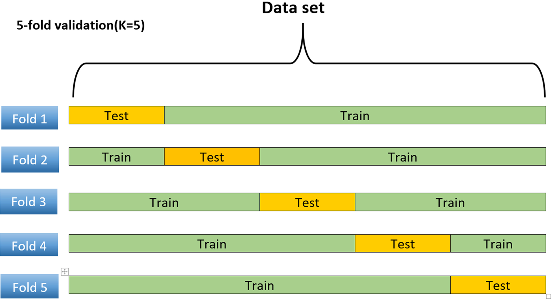
Data set with 5-fold cross-validation to evaluate classifiers. The orange cell shows the 20% of the testing set, and the green cells show the training set, which is 80% of the whole data set.
RESULTS
Experiment and results on region-based features
In this section, we have two objectives. First, identify the best classifiers and evaluate the features’ relevance. Figure 13 illustrates the pipeline of steps in 5 experiments. Each experiment will be examined in detail.
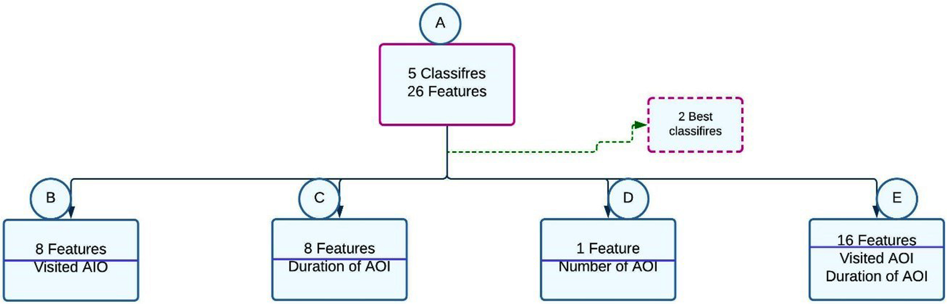
5 experiments pipeline architecture.
Experiment A used 26 features to select the best classifiers. Experiment B evaluates the relevance of “visited AOI” features. Experiment C evaluates the significance of the “duration of AOI” features. Experiment D evaluates the unique feature “ number of AOI.” Finally, experiment E evaluates the relevance of the combination of “visited AOI” and “duration of AOI” features.
We trained 5 classifiers (LR, k-nearest neighbors (K-NN), SVM, RF, and decision tree) on all features in experiment A. The results are presented in Table 3. SVM and Logistic regression have the highest values for the presented metrics (80% and 78.33% accuracy, respectively), and the K-NN shows the lowest value with 68.33% accuracy.
Experiment A with 5 different classifiers on all 26 features with 5-fold cross-validation. (RF stands for Random Forest and DT stands for Decision Tree
For experiment B, we chose two classifiers with the highest accuracy from the previous analysis, SVM with an accuracy of 80% and logistic regression with 78.33% accuracy were the best classifiers, respectively. For this step, we used only eight features out of our twenty-six visited areas of interest (visited AOI). These features had values between zero and three (0≤N≤ 3).
Therefore, feature scaling was not required (standardization) for this group of features. logistic regression gave 66.67% accuracy in both HC&AD, while SVM had better results with 76.67% accuracy for both HC&AD (see Table 4). Since the standard deviation was 0.00%, the mean accuracy for each 5 different fold was the same 66.0%.
Experiment B: LR and SVM classifiers on 8 features (visit AOI) with 5-fold cross-validation
For experiment C, we applied SVM and logistic regression classifiers to another eight features: the duration of time spent for each region (Duration of AOI). The results are presented in Tables 5 and 6. SVM shows higher values than logistic regression, with 73.33% for both AD and HC without standard scalar and 75.00%.
Experiment C: LR on 8 features (duration of AOI) with 5-fold cross-validation (W stands for standard scalar, and WO stands for without standard scalar
Experiment C: SVM on 8 features (duration of AOI) with 5-fold cross-validation validation (W stands for standard scalar, and WO stands for without standard scalar
For experiment D, we used one feature (Number of AOI). Table 7 shows the result of our two classifiers (logistic regression & SVM) with five-fold cross-validation. SVM shows higher values than logistic regression with (73.33% and 68.33% accuracy respectively).
Experiment D: LR and SVM classifiers on 1 feature (Area of AOI) with 5-fold cross-validation
For our last experience, E, we again applied two classifiers (SVM & Logistic regression) on sixteen features we separately analyzed in our previous experiments (Visit AOI & Duration of AOI). The results are presented in Table 8. SVM and logistic regression have the same results with 75% accuracy.
Experiment E: LR and SVM classifiers on mixed of sixteen features (Visit of AOI & Duration of AOI) with 5-fold cross-validation
We investigated the performance of the classifiers on various features. Thus, features with distinctive characteristics such as time duration, the number of areas of interest (AOI), and frequency of visited AOIs were analyzed. Our experiments show that SVM outperforms the logistic regression classifier in terms of accuracy. The highest accuracy associated with SVM (80%) was obtained in our first experiment with all twenty-six features. Logistic regression did not perform well and had the lowest accuracy on AOI duration (60%).
Experiment and results on trajectory-based features
In this section, we explored two sets of features based on trajectory. In the first experiment, we use the individual sub-distances r i as features. In the second experiment, we used r i as a feature.
Three to 6 divisions were applied for feature extraction and classification with LR and SVM. The result of these two classification approaches is almost identical (Table 9). The highest mean accuracy is associated with SVM (55%) with 3 division and extracted 6 features.
Trajectory analysis with LR classifier on individuals
Trajectory analysis with SVM classifier on individuals
DISCUSSION
Eye movement information plays an essential role in detecting AD. Medical findings show that people with AD have different eye-movement patterns compared to HC. However, using a patient’s eye movement for diagnosing at early steps is challenging.
The main goal of this work was to classify the probable AD and HC individuals by analyzing their points of gaze with the given transcripts and audio, which corresponded with the CT picture description task for AD diagnosis. In pursuit of this goal, we identified multiple regions in the CT picture that captured people’s attention by analyzing their descriptive speech. The identified regions were aligned with the time duration of the words they used.
As reported in Table 11, the total time spent describing the picture differs between the two groups (AD and HC). Our result shows that AD group spent more time than HC people representing the picture.
Total time spending for describing the whole picture
According to Table 12, our result shows that AD people spent more time on the virtual region (301.010 s). While HC individuals spent much less time on that region (16.481 s), HC participants seemed more focused on what they spoke about in each region. Moreover, there are noticeable differences between the time duration associated with each region. In general, AD people talked a lot more about some specific regions, for instance, VR, compared to the other regions. Thus, the variance or divergence of time spent on each region is more than HC participants. For four out of eight regions, AD participants talked over 300 s while HC participants mostly did not spend more than 262 s. Region 1 was one of the most interesting regions for AD, while it is one of the lowest regions of interest for HC.
Average time spent for each region in seconds
In region 1 (the woman), AD people spent more time (343.0415 s). In comparison, HC people among all regions spent more time on region 6 (the window). This shows a greater interest in details for the HC group since the backyard is not the focus point of the CT picture. AD people generally spent more time than HC describing the CT image (1961.75 s, Table 11). Table 12 shows the average time spent in each region for two groups of participants 30 HC and 30 ADs.
As shown in Fig. 14, AD people spent more time and attention on the virtual region (shown with blue color). While HC individuals (showed with orange color) spent more time in the region of 6. The region, 6 in the CT, represents the window and outside (yard, garage, bushes, etc.). It illustrates differences for region 7, region 5, and region 1.
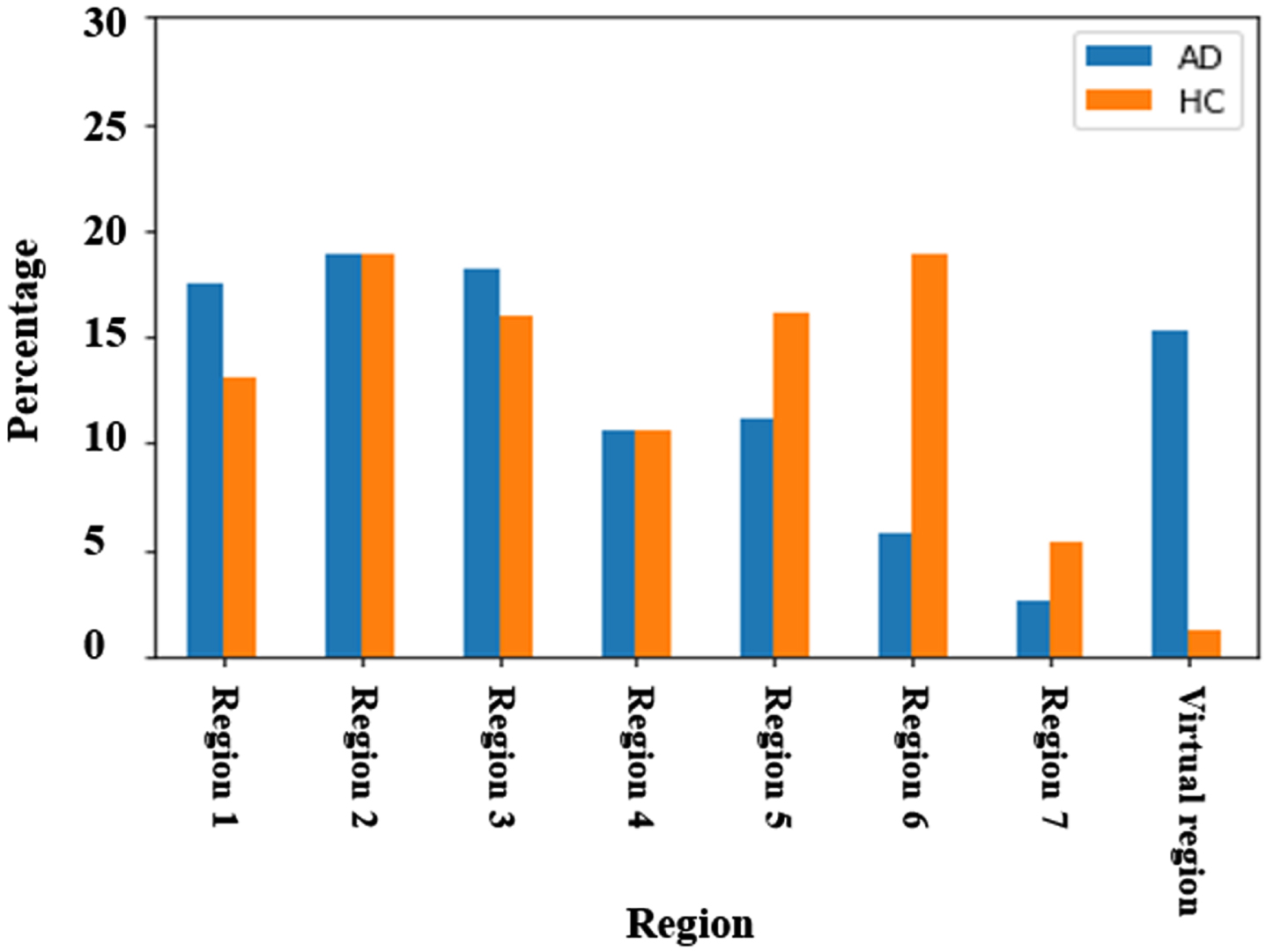
Percentage of total duration time on AOI for each group (AD and HC).
We also did a correlation analysis of features, reported in Table 13. The correlation matrix shows that AD people paid less attention to some regions than HCs. The highlighted values number of AOI and visited AOI in Table 13 can be interpreted as HC are 48% and 47% more likely to speak about more regions. AD individuals are more likely to speak about non-represented objects or characters (AOI VR is –36%).
Correlation matrix. Positive numbers in this table show probability of HC and negative values show the probability of AD
This method targets to classify the probable AD and HC individuals by analyzing their points of gaze, to develop a method for diagnosis of AD. In this context, the non-invasive and cost-effective nature of the method becomes crucial.
Firstly, our method does not require the use of expensive equipment such as an eye tracker. While eye-tracking devices are commonly used in dementia research, they can be costly and may pose a financial burden, especially for healthcare facilities with limited resources. By developing a method that does not rely on such specialized equipment, we eliminate the need for additional expenses and make the diagnosis more accessible.
Secondly, the method we propose avoids the need for imaging techniques like MRI. While MRI is a valuable tool for diagnosing various medical conditions, it can be expensive and often requires specific facilities and expertise. By focusing on early-stage diagnosis, which may not necessarily involve significant structural changes in the brain, we can bypass the need for MRI and its associated costs. This makes the method more affordable and readily applicable, especially in regions or healthcare settings where access to advanced imaging technologies may be limited.
One limitation of this work was the lack of data variations. Although the Pitt Corpus is public and available, the Picture Description task standard set is composed of pictures describing various scenes. The method should then be adapted to each new image.
Also, geographical and linguistic variations for data collection (the recorded transcript and audio) might help to come up with a more general solution. Therefore, in our future work, we will consider other samples and collective data from different sex, ethnicity, continent, and even language.
As it is, our method is not fully automated. Our next step will be to automate the association between the transcripts and the region. Furthermore, a complementary approach for the combination uses an accurate eye-tracker tool and word tracker.
This research offers a novel approach for feature extraction and selection for classifying the AD and HC participants using the Pitt Corpus data set on the cookie theft picture. The 80% accuracy achieved with SVM suggests that our approach is comparable with the results of methods that tackle the same problem (Fraser et al. [15] and Lagun et al. [17]) applied SVM with 86% and 87% accuracy, respectively; both of them used eye tracker tool, but without having an eye tracker tool.
In conclusion, contrary to other expensive or invasive methods, this study introduces a machine learning-based non-invasive, and economical approach that paves the road for clinicians and researchers for early AD diagnosis. Additionally, the proposed method could be seen as a complementary approach to the one that used linguistic features [24].
Footnotes
ACKNOWLEDGMENTS
The authors have no acknowledgments to report.
FUNDING
This research is supported by a grant from the NSERC (Natural Sciences and Engineering Research Council of Canada) RGPIN-2018-05714.
CONFLICT OF INTEREST
The authors have no conflict of interest to report.
DATA AVAILABILITY
All the results were added in the manuscript and if any extra data needed the corresponding author will provide it.