Sizing by SQP optimization of an electrical drive: Application to a switched capacitor connected to a permanent magnet synchronous generator

Abstract

The paper deals with the design by optimization in pre-sizing step of a drive system that combines a switched capacitor system and a permanent magnet synchronous machine (PMSM). The sizing of the converter and the machine are considered strongly dependent due to the series quasi-resonant topology. The system modelling is based on a semi-analytical approach validated by finite element (FE) simulations. It involves an analytical modelling of the electrical machine and a numerical time solving of the electrical circuit sub-model because of the natural switching events of diodes. The optimization is carried out by SQP (Sequential Quadratic Programming). The model gradients are computed combining mathematical laws, symbolic derivation and automatic differentiation. Finally, trade-offs and gains on the machine power density, the magnet volume and the efficiency are investigated through a Pareto approach.

Keywords

Analytical modelling permanent magnet synchronous machine flying capacitor interface model derivation SQP

1. Introduction

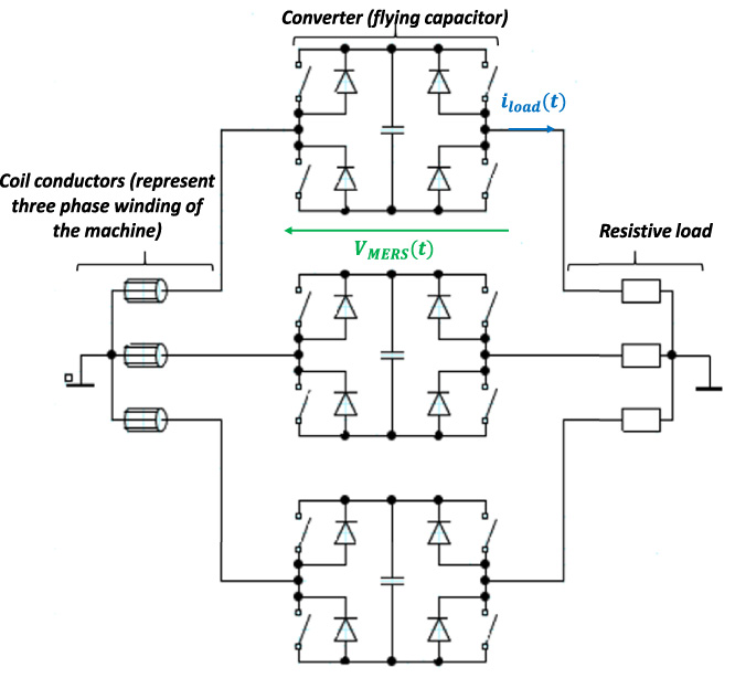
Nowadays, power converters that use quasi-resonant operating mode are numerous and are covering a wide application domain from small power energy systems to large power systems as wind turbine systems. In [1–3], the authors investigate one of those converters named Magnetic Energy Recovery Switch System that works like a quasi-resonant dimmer power circuit. This can be connected in series with a Permanent Magnet Generator and is suitably used to control the output power supplied to the load. Focusing on the same application case depicted in Fig. 1. In the paper, the authors focuses on how this flying capacitor type converter connected in series with a synchronous generator is modifying the design of the machine and the power electronics components. In this so-named pre-sizing step, the principal goal is to evaluate the expected gain on the machine by associating it to a flying capacitor converter and locate the compromises. It is therefore important to have a systemic approach in order to have an overview. Likewise, the use of medium and low fidelity modelling as well as gradients based algorithms is recommended in order to quickly browse all of the possible solutions included in the study space. Subsequently, the choice of SQP algorithm is made for optimisation. It allows solving of inverse problem with large input number with equality and inequality constraints and is able to converge very rapidly aiming to the gradients.

Fig. 1.

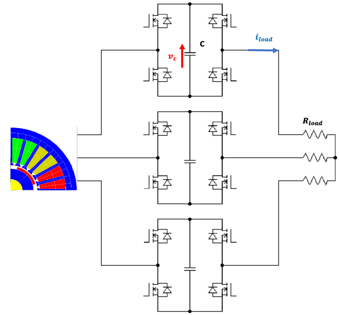
Electrical drive of studied application.

After presenting the global sizing model, the paper splits up the modelling into two sub-models: the machine model and the electrical drive model.

Firstly, the modelling of the machine is detailed. It involves homogenisation step to describe the machine topology. It results that teeth and slots are no more considered. It follows that some local outputs as magnetic flux densities in teeth and back-iron, electromotive forces, etc. have to be retrieved from homogenised values. Secondly, the power electronics modelling based on state systems is presented. The solving process detailed in [4] is no more described and focus is made on how outputs and their derivatives in respect to the inputs are calculated for both sub-models.

Thirdly, optimization results are presented using the Pareto front considering the trade-offs between the total losses versus the volume of the machine. Optimal sizings are then compared to the reference one considering that the output power and the specifications are fixed. Then, Pareto results are extended to specific ones aiming to demonstrate how flying capacitor converters could also change the design trade-off to reduce the permanent magnet volume of the machine.

2. Global sizing model

The global sizing model of the drive system is divided into sub-models as depicted in Fig. 2: the electrical machine sub-model and the power electronics one. The modelling of the machine aims to compute: the flux densities, the magnetic and Joule losses that are considered as outputs from geometric sizes and materials properties that are inputs. It must be noticed that other inputs have to be calculated by the power electronics sub-model as the current values (required to compute flux densities and Joule losses). Knowing that a loop appears between the inputs and the outputs of the two sub-models, it is worth to observe that there is no implicit solving. In the power electronics sub-model, the machine is represented by a linear equivalent electrical circuit model. Therefore, current value (rms and peak) are no more required and the equivalent electromotive force and the synchronous inductance are calculated without those.

Fig. 2.

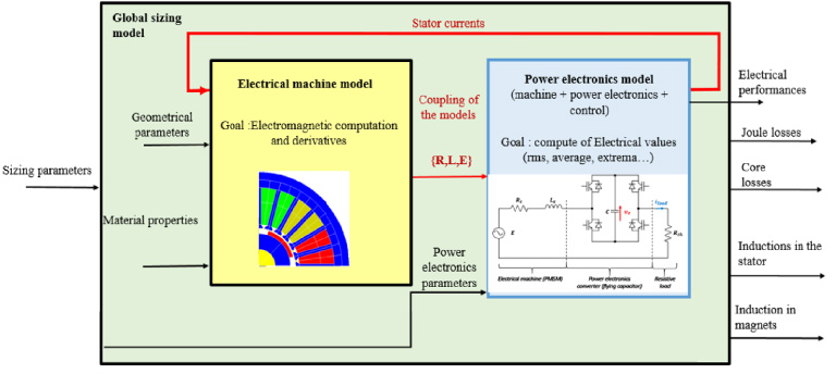
Architecture of the global sizing model of the electrical drive.

Electrical waveforms are computed by the power electronics sub-models deducing: rms, average and peak values of the currents and voltages. The power output feeding the load is computed through electrical waveforms so harmonics effects and load angle changes are considered. Finally, as described in the following sections, all the derivatives of the outputs according to the inputs are also calculated by the sub-models.

3. Electrical machine modelling

The initial electrical machine is an existing one, described in [5]. It is a surface mounted permanent magnet synchronous generator with two pole pairs, 24 stator slots and full-pitch winding. It will be used both to validate the modelling and to estimate the reference operating point given by the generator supplying the load without power electronics converter. All the specifications of the machine are given in Table 1 and the geometric parameters are described in Fig. 3.

Table 1
Parameters of the studied permanent magnet synchronous machine

Geometrical parameters

Rotor radius (R₁) [mm] 25.89

Stator radius (R₄) [mm] 75

Average teeth thickness (b_ts) [mm] 3.62

Magnets thickness (h_m) [mm] 3.14

Magnet pole’s opening angle (𝜓_m) [°] 60

Slot deep (h_ss) [mm] 32.5

Back-iron thickness (h_sy) [mm] 12.5

Air gap (GAP) [mm] 1

Active length (L) [mm] 160

Physical parameters

Number of turn per slot (N) 5

Residual induction of the magnet [T] 1.1

Relative permeability of the magnetic circuit material (μ_r) 5600

Fig. 3.

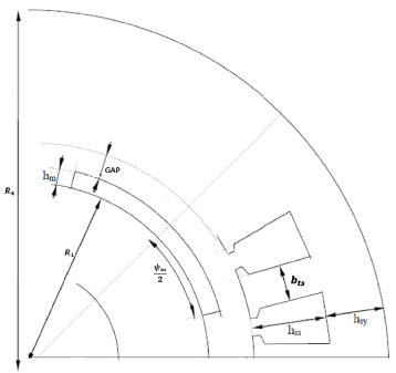
Geometry of one pole of the studied machine.

The aim of the design by optimization is to guide the engineers in the predesign phase. The goal is to evaluate the expected gain on the machine by associating it to a flying capacitor converter. High fidelity modelling (based on finite element (FE) simulation) used in design phase to reduce time-to-market and prototyping steps are not considered. In pre-design step, when engineers have to make choices, evaluating solutions and to defined specifications, focus is so made on a medium and low-fidelity modelling such as magnetic reluctance circuit [6] and analytical harmonic modelling approach [7–9]. These modelling enable to compute the Jacobians and allowing the use of gradients based algorithms in optimizing framework.

Analytical harmonic modelling is chosen here because it basically involves an homogenization step instead of a meshing one used in the other modelling approaches. It allows to describe various complex geometry by only one, replacing cut edges as slots, teeth and non-consequent permanent magnets by only equivalent concentric ring forms [7].

This modelling was historically applied to various permanent magnet magnetization patterns (radial, parallel or tangential) and was recently improved to step forward both slotting effects and saturation [8,9]. In the authors viewpoint, it follows that a modelling that could described in a parametric way various topologies of machines is attractive and should be supported.

It could also be noticed that after solving the field on annular forms, teeth and back-iron flux densities, demagnetizing field on magnets are suitably estimated even if geometrical effects were not precisely described due to the homogenization step.

In addition, the analytical modelling is based on the following hypothesis:

–

not taking into account 3D effects.

–

the initial geometry of the machine is replaced by concentric rings described by homogenised areas representing different magnetic regions, as described in Fig. 4.

–

the currents in the stator are represented by a linear current density at the stator inner diameter, equivalent to the ampere turns created by the coils and whose spatial distribution can be defined by: $\begin{eqnarray}k_{s}({\varphi})=\mathop{\sum }_{n_{s}=0}^{N}K_{s}{k_{w}}_{n_{s}}e^{in_{s}{\varphi}}\end{eqnarray}$ (1) where n_s is the spatial harmonic rank, k_w denotes the associated winding factor and K_s denotes the current source.

–

Rotor and stator magnetic materials are the same and described by linear magnetic behaviour of relative permeability μ_r = 5600; the magnetic flux densities in teeth, back-iron and rotor will be estimated a posteriori and constrained during optimization process.

–

the permanent magnets are treated as a homogeneous medium depicted by a relative permeability μ_rpm and a radial remanent magnetisation, continuously described by a Fourier series: $\begin{eqnarray}M({\varphi})=\mathop{\sum }_{n_{r}=1}^{\infty }\frac{1}{n}K_{pm_{n_{r}}}e^{in_{r}{\varphi}}\end{eqnarray}$ (2) where n_r is the spatial harmonic rank, K_pm the associated harmonic amplitude of the magnetization given for radial magnetization pattern by: $\begin{eqnarray}K_{pm_{n_{r}}}=-\frac{2pM_{r}}{{\pi}}\cdot \sin \left(\frac{{\pi}n_{r}{\beta}}{2p}\right)\cdot \left(\sin \left(\frac{n_{r}{\pi}}{2p}\right)-\sin \left(\frac{3n_{r}{\pi}}{2p}\right)\right)\end{eqnarray}$ (3) where p is the number of pair poles per phase and 𝛽 is the opening pole angle.

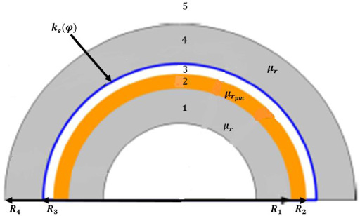
As depicted in the literature [7,8], the magneto static field equations are reduced to Poisson and Laplace partial differential equations of the magnetic potential $\overrightarrow{A_{z}}(r,{\varphi})\overrightarrow{u_{z}}$ in cylindrical coordinates, respectively in the permanent magnets and in all other areas: the magnetic stator and rotor, and the air-gap. The solutions of those equations are symbolically obtained by the Fourier method and are expressed as sum of spatial harmonics:

Fig. 4.

Modelling of the electrical machine: geometric simplification.

$\begin{eqnarray}A_{z}^{(m)}(r,{\varphi})=\mathop{\sum }_{n=1}^{\infty }(a_{n}^{(m)}r^{n}+b_{n}^{(m)}r^{-n})e^{in{\varphi}}.\end{eqnarray}$ (4) The solution of the Poisson equation in the magnet is given by: $\begin{eqnarray}A_{z}^{(2)}(r,{\varphi})=\mathop{\sum }_{n=1}^{\infty }\left(a_{n}^{(2)}r^{n}+b_{n}^{(2)}r^{-n}+\frac{{K_{pm}}_{n_{r}}r}{1-n^{2}}\right)e^{in{\varphi}}\end{eqnarray}$ (5) where $a_{n}^{m}$ and $b_{n}^{m}$ are coefficients that are found using the magnetic field interface conditions between areas denoted by over script (m): rotor (1), Permanent Magnet (PM) (2), air-gap (3) and stator (4) and air (5). It follows that only eight coefficients are used to define the solutions in all the areas, $b_{n}^{(1)}$ and $a_{n}^{(5)}$ remaining zero due to boundary conditions at r = 0 and r = ∞. Interface conditions for radial magnetic flux density and orthoradial field strength are finally used to define eight linear equations: $\begin{eqnarray}\displaystyle \text{} & \text{} & \displaystyle \left(\begin{array}{@{}cccccccc@{}}\displaystyle \frac{{\mu}_{\text{rpm}}}{{\mu}_{r}} & -1 & R_{1}^{-2n} & 0 & 0 & 0 & 0 & 0\\[10.0pt] \displaystyle 0 & 1 & -R_{2}^{-2n} & -{\mu}_{\text{rpm}} & {\mu}_{\text{rpm}}R_{2}^{-2n} & 0 & 0 & 0\\[5.0pt] \displaystyle 0 & 0 & 0 & u_{r} & -{\mu}_{r}R_{3}^{-2n} & -1 & R_{3}^{-2n} & 0\\[5.0pt] \displaystyle 0 & 0 & 0 & 0 & 0 & 1 & -R_{4}^{-2n} & {\mu}_{r}R_{4}^{-2n}\\[5.0pt] \displaystyle 1 & -1 & -R_{1}^{-2n} & 0 & 0 & 0 & 0 & 0\\[5.0pt] \displaystyle 0 & 1 & R_{2}^{-2n} & -1 & -R_{2}^{-2n} & 0 & 0 & 0\\[5.0pt] \displaystyle 0 & 0 & 0 & 1 & R_{3}^{-2n} & -1 & -R_{3}^{-2n} & 0\\[5.0pt] \displaystyle 0 & 0 & 0 & 0 & 0 & 1 & R_{4}^{-2n} & -R_{4}^{-2n}\end{array}\right)\cdot \left(\begin{array}{@{}c@{}}a_{1}^{n}\\[5.0pt] a_{2}^{n}\\[5.0pt] b_{2}^{n}\\[5.0pt] a_{3}^{n}\\[5.0pt] b_{3}^{n}\\[5.0pt] a_{4}^{n}\\[5.0pt] b_{4}^{n}\\[5.0pt] a_{5}^{n}\end{array}\right)\nonumber\\ \displaystyle \text{} & \text{} & \displaystyle \quad =\left(\begin{array}{@{}c@{}}\displaystyle \frac{K_{pm_{n}}R_{1}^{1-n}}{n(1-n^{2})}\\[10.0pt] \displaystyle \frac{-{K_{pm}}_{n}R_{2}^{1-n}}{n(1-n^{2})}\\[10.0pt] 0\\ 0\\ \displaystyle \frac{K_{pm_{n}}R_{1}^{1-n}}{1-n^{2}}\\[10.0pt] \displaystyle \frac{-{K_{pm}}_{n}R_{2}^{1-n}}{1-n^{2}}\\[10.0pt] 0\\ 0\end{array}\right)\quad \text{or }\left(\begin{array}{@{}c@{}}0\\ 0\\ \displaystyle \frac{-{K_{s}}_{n}{\mu}_{r}}{nR_{3}^{1-n}}\\[13.0pt] 0\\ 0\\ 0\\ 0\\ 0\end{array}\right)\end{eqnarray}$ (6) where R₁, R₂, R₃, R₄ are radius delimiting areas as described if Fig. 4.

The linear system (6) is written as matrix one CX = D and according to superposition property of linear system, the source vector D is splitted up, depending on the source taken into account. The corresponding unknown coefficients are then denoted by subscript “r” for rotor source (magnets) and subscript “s” for stator source (currents).

As rotor and stator saliencies are not taken into account due to homogenisation approach and according to the Curie principle, the harmonic contents to be considered are those of the linear current density (2) and the magnetisation (1) in the PM [7].

3.1. Calculated outputs

Knowing the magnetic potential values in the homogenised areas, a backward calculation from the homogenisation step are applied and the local magnetic flux densities values are estimated in the machine.

Fig. 5.

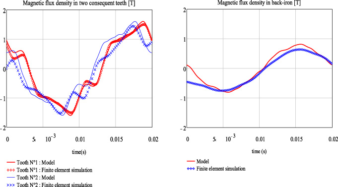
Comparison of magnetic flux densities in teeth and back-iron issue from analytical model and finite element simulation for the initial machine.

The magnetic flux per pole is calculated using the circulation of the magnetic potential around the arc defined by the stator inner radius and the pole angle π∕p: $\begin{eqnarray}{\phi}_{pole}=\left(A^{(4)}(R_{3},{\varphi}_{i},t)-A^{(4)}\left(R_{3},{\varphi}_{i}+\frac{{\pi}}{p},t\right)\right)\cdot L\end{eqnarray}$ (7) where L is the active length of the machine, φ_i is the reference angle of the pole defined by the rotor position, A⁽⁴⁾ denotes the total potential due to both rotor and stator sources $A^{(4)}(r,{\varphi})=A_{r}^{(4)}(r,{\varphi}+{\alpha})+A_{s}^{(4)}(r,{\varphi})$ , 𝛼 denotes the load angle.

The magnetic flux flowing in the back-iron is then estimated considering that the flux per pole split up into the two consequent poles. Then the average magnetic flux density is calculated according to the back-iron cross section and will be constrained in the optimization step (see Section 6).

The magnetic flux in the teeth are estimated in the same way, considering the pitch angle. To validate our approach, magnetic flux density in two consequent teeth and in the back-iron are compared to FE simulation results for the initial machine in Fig. 5 and shows good agreements between waveforms with errors less than 15% on the peak values and 31.5% on the rms derivatives that are quantities used to compute magnetic losses. It demonstrates that the modelling of the machine using simple geometry remains relevant at the scale of teeth when using reverse homogenisation step to estimate local flux densities.

When the magnetic flux densities in the teeth and the back-iron, and their time derivatives are well calculated, the magnetic losses in the stator are estimated by the Bertotti model. This one is based on physical meaning that losses could be separately estimated into hysteresis, Eddy current and excess losses [10]. The magnetic loss density in W/m³ is then easily calculated by: $\begin{eqnarray}P_{losses}=\frac{1}{T}\cdot \int _{0}^{T}\left(k_{h}fB_{m}^{2}+\frac{{\sigma}d^{2}}{12}\left(\frac{dB(t)}{dt}\right)^{2}+k_{e}\left|\frac{dB(t)}{dt}\right|^{\frac{3}{2}}\right)dt.\end{eqnarray}$ (8) As depicted in [5], the magnetic cores are made of M800-65A electrical steel sheets with the coefficients: k_h = 279.81; σ = 4 ⋅10⁻⁶; k_e = 1.28.

When designing permanent magnet actuators, one has to consider the field strength in the magnet to avoid their demagnetization. In our application case, magnetic field in the magnets could be increased by the reduction of their thickness and by increasing the stator current. It is so very important to estimate the magnetic flux density in the magnets in the optimization step. 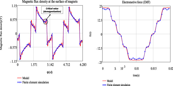According to our modelling, the radial flux density is easily deduced from the magnetic potential in the magnet by: $\begin{eqnarray}B_{r}(r,{\varphi})=\frac{1}{r}\frac{\partial A_{2}(r,{\varphi})}{\partial {\varphi}}.\end{eqnarray}$ (9) The flux density is then estimated depending in the load angle and where the field due to the stator is opposite to the one of the magnet, describing the worst case to be constrained. Figure 6 shows the radial flux density in the magnet for the reference machine and the circle gives the retained value.

Fig. 6.

Comparison of electromotive force and flux density in the permanent magnets obtained by analytical model and finite element simulation, for the initial machine.

3.2. Electrical equivalent circuit modelling

In order to consider the machine in the time simulation involved by power electronics and system modelling, the previous modelling is reduced to an electrical equivalent circuit. Assuming that the machine has no salient poles, and that the saturation is no more acting beyond the slot wedges, the machine is represented by the well-known Behn-Eschenburg circuit per phase (assuming balanced 3 phases).

The electromotive force (emf) denoted by the voltage source E is deduced from the magnetic flux due to permanent magnets (𝜙_r) and viewed by the coil considering Eq. (7) with $A_{r}^{(4)}$ in respect of A⁽⁴⁾. So, it is estimated considering the difference of the magnetic potential calculated at the slot opening. In the case of the initial machine with two slots per pole per phase, it is given by: $\begin{eqnarray}\displaystyle E(t) & = & \displaystyle Np∼{\omega}\left(A_{r}^{(4)}(R_{3},{\varphi}_{i},t)-A_{r}^{(4)}\left(R_{3},{\varphi}_{i}+\frac{{\pi}}{p},t\right)+A_{r}^{(4)}\left(R_{3},{\varphi}_{i}+\frac{2{\pi}}{24},t\right)\right.\nonumber\\ \displaystyle \text{} & \text{} & \displaystyle -\left.A_{r}^{(4)}\left(R_{3},{\varphi}_{i}+\frac{2{\pi}}{24}+\frac{{\pi}}{p},t\right)\right)\cdot L\end{eqnarray}$ (10) where, N is the number of turns per slots, ω is the electrical pulsation.

The electromotive force is depicted in Fig. 6 considering harmonics up to 17th rank and show good agreement with FE simulations.

In the same way, the inductance is deduced from the total magnetic flux due to the current flowing in the stator and viewed by the coil divided by the current itself. It is expressed by 𝜙_s replacing here A⁽⁴⁾ by $A_{s}^{(4)}$ in Eq. (7). The synchronous inductance is thus related to the cyclic inductance and is estimated by: $\begin{eqnarray}L_{s}=\frac{3}{2}\frac{N{\Phi}_{s∼max}}{I_{\max }}\end{eqnarray}$ (11) where Φ_s max and I_max are respectively the maximum value of the magnetic flux and the current flowing in the coil.

It should also be noticed that all the fluxes are estimated at the stator inner radius. It results that the leackage flux between teeth are not taken into account and may cause some inaccuracies when estimating the average flux in teeth and the synchronous inductance. The error is about 1.7% for the initial machine with L_s = 390 μH estimated by the model compared to L_s = 397 μH calculated by FE simulations.

Finally, the resistance R_s is only depending on the stator sizes. To validate the resistance calculation, FE simulations are not relevant (2D and the winding not precisely described in slots) and the considered value is the same in both modelling. Finally, the stator Joule losses is simply calculated using: $\begin{eqnarray}P_{\text{Joule}}=3RI_{\text{rms}}^{2}.\end{eqnarray}$ (12)

3.3. Derivatives related to the machine modelling

Derivatives of all the outputs (P_losses, P_Joule, L_s, flux densities, …) according to the inputs (geometric parameters, magnetic properties) are all deduced from those of magnetic potential coefficients $a_{n}^{(m)}$ by chain rules.

Assuming the matrix equation CX = D and denoting P the vector of all the input parameters, the derivative of the matrix equation CX = D with respect to P, is: $\begin{eqnarray}C\frac{\partial X}{\partial P}=\frac{\partial D}{\partial P}-X\frac{\partial C}{\partial P}.\end{eqnarray}$ (13) This new matrix equation has the same first member matrix C than the initial one (6). So, the LU decomposition used to solve (6) is simply re-use to solve (13) enabling to compute the derivatives without large additional computational and so time-consuming effort [11].

4. Power electronics modelling

4.1. Model

The power electronics converter is composed of three single-phase full bridge with flying capacitor as depicted in Fig. 1 [2]. The whole system consisting of the generator and the converter is assumed to operate in a three-phase balanced mode. It results that only an equivalent single phase is then considered.

The main objective is to compute the electrical waveforms at the switching frequency so switches and capacitor are assumed ideal. It results that the converter can be seen as a capacitor connected in one direction or in the other depending of the control or even as a short-circuit bypassing the capacitor when it is fully discharged [1]. It define three possible circuit topologies during an operating period as shown in Fig. 7 from which three different state systems are derived.

Fig. 7.

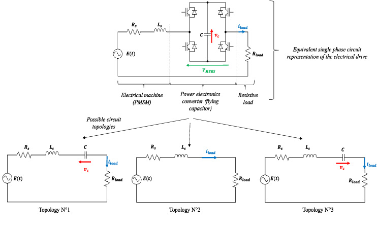
Equivalent single-phase circuit representation of studied electrical drives and state circuit topologies.

The state systems of circuit representations are solved in time domain using Runge–Kutta method (RK44) combined with an adaptive time step-size control strategy [4]. Tests on control to detect hard switching events and test on zero crossing of the voltage across the capacitor to detect soft switching of diodes are implemented to manage the solving process between the state systems.

The outputs of the model are extrema, rms values of currents and voltages, as well as average values. They are computed on one operating period, at steady state.

The integral expressions involved in the computation of the rms and average values, are carried out using trapeze method. Extrema are found using an algorithm based on tests on the corresponding variables.

4.2. Derivatives

Paper [4] discusses methods to compute the Jacobian of a time model of power electronics converters in the aim of sizing them using gradients based optimization. The method described in [12] is retained and a new state system that involves both state equations and their derivatives with respect to sizing parameters (E, L_s, R_s, R_ch) is derived. It allows solving the state variables and their derivatives in the same solving process.

Then, derivatives of outputs are obtained using several mathematic methods. The limit of the approach is the fact that derivatives according parameters formulated in a non-continuous way (control variables) are obtained using finite difference.

5. Implementation

The global sizing model has been implemented using CADES framework [13]. A specificity of CADES is its ability of coupling different models by exploiting the concept of software components. The electrical machine model and power electronics models, as well as the computation of their derivatives are implemented in Java language. Other analytical equations are defined for the coupling of models and the Joule and core losses. They are implemented in SML language and there derivatives are obtained using the automatic differentiation tool Adol-C implemented in CADES (Fig. 8). Optimizations are carried out with SQP (VF-13 from Harwell library).

Fig. 8.

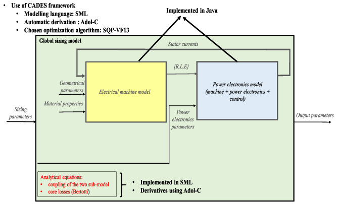
Global sizing model: Implementation in CADES Framework.

6. Optimization results and discussion

6.1. Specifications

The pre-design steps aims to determine the trade-offs that are acting on the sizing of the machine when it is driven by a flying capacitor converter. As previously said, the flying capacitor is suitable to boost the voltage across the machine by compensating the reactive energy and so hiding the drop voltage across the synchronous inductance. It results that, on one hand, the current and voltage could be higher, increasing the output power; or, on the other hand, the electromotive force could be smaller for the same output power. We choose to evaluate the design trade-off on the second way and we focus on reducing the volume of the machine under the constraint of constant power output. The output power is constrained and defined by the maximum output power supplied by the reference machine (3.6 kW) (Initial machine in Table 2) [5] connected to a resistive load without flying capacitor depicting the reference study case. The load resistance remains fixed during the optimization steps (R_load = 0.12 Ω), as well as the mechanical speed (1500 rpm). Therefore, mechanical losses are identical for the two machine (the initial machine and the optimized one) and are not taken into account in this study.

Table 2
Optimization results

Input parameters

Initial machine Optim No 1 Optim No 2 Optim No 3

Magnet thickness (h_m) [mm] 3.14 5 1.49 1.12

Pole’s opening angle (𝜓_m) [°] 60° 75° 61° 70°

External stator radius (R₄) [mm] 75 60.6 60.6 75

Back-iron thickness (h_sy) [mm] 12.5 10.3 1.7 5.64

Tooth width (b_ts) [mm] 3.62 3.77 2.5 4

Slot depth (h_ss) [mm] 32.5 21 44.25 41.37

Number of turns per slot (N) 5 3 11 5

Power electronics capacitor (C) [mF] 31.3 1.97 39.95

Power electronics control parameter (δ) 0.35 0.4 0.29

Output parameters

Electrical performances

Maximum voltage across capacitor [V] 6.9 97 24.15

rms current in the capacitor [A] 63.4 58.4 100.2

rms current in the machine [A] 100.2 100.2 100.2

Maximum current in the machine [A] 145 118.8 120.4 156.14

Current density j [A/mm²] 3.76 4.38 6.9 2.92

Power losses

Joules losses [W] 133 96.3 551 103.4

Core losses [W] 47 58.9 64.3 76.6

Total losses [W] 180 155.2 615.3 180

Electromagnetic performances

Maximum induction in teeth [T] 1.6 1.8 1.8 1.8

Maximum induction in back-iron [T] 0.81 1.4 1.4 1.15

Induction in magnet [T] 0.41 0.85 0.39 0.25

Dimensions of machines

Machine volume [L] 2.83 1.84 1.84 2.83

Permanent magnet volume [L] 0.0144 0.027 0.00328 0.00583

The design problem has ten input parameters including six geometrical sizes (magnet thickness, pole opening angle, external stator radius, back-iron thickness and tooth width and slot depth), the number of turns per slot and the current density and two parameters associated to the converter (the capacitor value and the control angle). The active length of the machine is fixed because of the 2D modelling and the lack of describing the end-windings effects. There are five outputs performances: the Joule and magnetic losses, the flux densities in the teeth and in the back iron and the machine volume. The flux densities are constrained to remain below 1.8 T in teeth and below 1.4 T in the back iron. The demagnetizing field in the magnet is estimated in the worst area of the magnet depending of the load angle of the machine. Its value is constrained to 0.1 T to avoid operating point close to the coercive field strength.

Two objectives are considered: the global volume of the machine (related to the power density because output power is fixed) and the total losses. So a Pareto strategy is used.

6.2. Pareto front building

The Pareto front is obtained by SQP optimisation minimizing the total losses according to 12 sampled values of the volume. These values are spread out in the range defined by the two limits of the Pareto front obtained from two optimisation: minimizing the total losses and minimizing the machine volume. The Pareto front is computed in approximatively 15 min on standard PC (Windows 10, core i5@2.6GHz, 4Go Ram).

Figure 9 presents this front. The initial machine (reference) appears in blue in the figure.

Fig. 9.

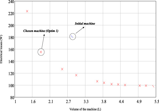
The Pareto front minimizing the total losses in the machine according to values the volume.

6.3. Chosen machine

It is valuable to compare the initial machine to the solution from the Pareto curve that offers a good compromise between objectives point circle on Fig. 9 and denoted by Optim No 1 in Table 2. The main difference between the two machines are summarized in Fig. 10.

Fig. 10.

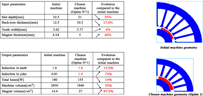
Comparison between the initial machine and the chosen solution (Optim No 1 in Table 2) from Pareto front.

The optimized machine exhibits a volume of 1840 cm³ (35% lower than the initial machine). The output power is fixed at 3.6 kW so power density is increased by 35% too. The thermal modelling is not considered here. So one as to notice that the thermal management should be more constrained considering the optimal machine with lower losses decreasing by 14% with an external surface reduced by 19%. However, in the other hand, the ratio between Joule and core losses changes significantly from 2.8 to 1.6 allowing re-considering the thermal management issue.

As expected, the flux densities are increased in the teeth (+12.5%) but mainly in the back-iron (+73%). Whereas the magnetic flux density values goes up, the core volume goes down. So, finally, the magnetic losses increase by 25%.

At the opposite, the Joule losses decreases by 28% because of the reduced number of turns per slot and of the lower sizes of the machine. The current density increases from 3.76 A/mm² (reference machine) to 4.38 A/mm, so, the slot area decreases by 48% while the current rms value is kept at 100 A. It should be noticed that the Ampere-turns per slot are reduced, so the magnetic field due to the stator coils is lower in the optimal machine than in the initial one. In addition, the permanent magnet thickness is increased by 59%, increasing the field due to the rotor source. The electromotive force (emf) is at the opposite reduced by 37% due to the lower number of turns per slot.

According to that, it is valuable to highlight that the phase-angle between the emf and the current is reduced as depicted in Fig. 11. The flying capacitor is able to change the current waveform and the phase-angle, with respect to the emf, i.e. the load angle to keep the output power constant. The converter is operating in a discontinuous mode where C is 31.3 mF and the control angle δ is 0.35. The voltage across the capacitor is low compared to the emf values and remains below 10 V as shown in Fig. 11 (Optim 1).

Fig. 11.

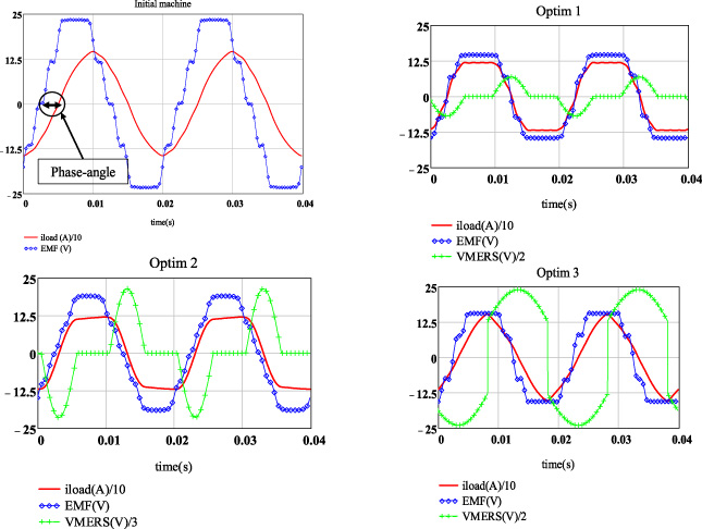
Comparison of waveforms for initial machine and optimums.

In order to validate the optimization results, finite element simulation of the complete drive system (PMSM connected in series with a flying capacitor) are carried out in a transient magnetic application with Altair Flux^TM software. Flux software is using field-circuit coupling: FE equations are coupled with circuit equations; the converter is defined using ideal switches and diodes as shown in Fig. 12 and the solution of the electrical circuit and magnetic field are solved simultaneously. It results that current and voltage waveforms are fully computed considering both FE simulation of the machine in magnetic transient application and considering the converter switching control. It allows comparing the waveforms to ones obtained in our models as shown in Fig. 13. It results that good agreements between both modelling is obtained with errors less than 10% on current and flux densities. The voltage across the capacitor of the converter is miscalculated due to bad zero-crossing detection because the time step is too large in the FE transient application. It also validate the robustness of the sizing model according to parametric variations.

Fig. 12.

Circuit diagram of the drive system in Altair Flux^TM.

Fig. 13.

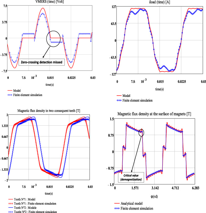
Comparison waveforms issues for analytical model and finite element simulation, for the optimal machine (Optim No 1 in Table 2).

6.4. Other solutions

Finally, the paper focuses on the volume of permanent magnets in the machine. When reducing the volume of the machine (Optim No 1 in Table 2) the volume of the magnets is increased by 87.5% up to 27 cm³ with respect of the initial machine. Two more optimizations are so made to minimize the volume of the magnets. One way is to set the volume of the machine to the one of the reduced machine (Optim No 1) and to minimize the magnet volume instead of the total losses. It results in a poor design (Optim No 2) where the losses are increased by 250% whereas the volume is reduced, leading to an important thermal issue. The other way is to choose to minimize the magnet volume and to set the total losses and volume at their initial values (Optim No 3), avoiding thermal issues. It results that the magnet thickness is greatly reduced down to 1.12 mm and the magnet volume is reduced by 60%. It is valuable to noticed that the flux density in the magnet is decreased to 0.25 T but above the lower limit: 0.1 T. In the same way, the use of the switched capacitor allows the reduction of the phase-angle between the electromotive force and the current as shown in Fig. 11 Optim No 3. It makes possible to provide the same power to load, despite the reduction of the amplitude of electromotive force, compared to the initial electrical drive. However, it can be noticed that the flux densities in airgap (due from one hand to the magnet and to the other hand to the current in stator) are well balanced, as shown in Fig. 14.

Fig. 14.

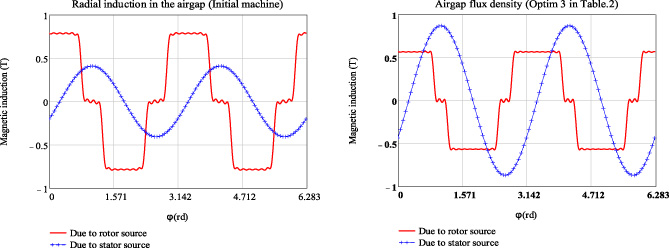
Comparison of radial induction created in the airgap for the initial machine and the optimal machine minimizing the volume of magnets (Optim No 3 in Table 2).

According to the converter, the capacitor value is 40 mF but the voltage is increased up to 24 V and the RMS current flowing in the capacitor is about 100 A in DC-offset mode.

7. Optimization results and discussions

The paper has proposed a complete model of an electrical drives. This model is spilt up in two sub-models: the machine model based on Maxwell equations and the electrical drive model based on ideal circuit representation. These models are faster than FEM element models or time simulation tools, and they implement their jacobian useful for SQP optimisations. Pareto front are obtained and discussed for the studied electrical drive.

In future works, for the studied drive, it will be interesting to precisely designing the converter for the operating point of the solution (optim No 4) in order to investigate a way that the flying capacitor could efficiently reduce the magnets volume.

References

Takaku

Homma

Isobe

Igarashi

Uchida

and Shimada

, Improved wind power conversion system using magnetic energy recovery switch (MERS), in: IEEE Industry Applications Conference, 2005, pp. 2007–2012.

Morel

Garbuio

Chazal

and Diarra

Z.D.

, Output power control of a surface mounted permanent magnet synchronous generator coupled with electronic capacitor system, in: XIII International Conference on Electrical Machines (ICEM), 2018, pp. 2269–2275. doi:10.1109/ICELMACH.2018.8507150.

Morel

Garbuio

Chazal

and Diarra

Z.D.

, Reduction of permanent magnet volume in PMSG using non-linear power conversion system, in: 9th International Conference on Power Electronics, Machines and Drives (PEMD), 2018.

Gerbaud

Diarra

Z.D.

Chazal

and Garbuio

, Obtaining the most exact Jacobian for the time modelling of a power electronics structures to be used by gradient optimization algorithms, in: 16th International Workshop on Optimization and Inverse Problems in Electromagnetism, 2021, pp. 103–104.

Meier

, Theoretical design of surface-mounted permanent magnet motors with field-weakening capability, Master thesis, Royal Institute of Technology department of Electrical Engineering Electrical Machines and Power Electronics, 2002.

Nguyen-Xuan

Dogan

Perez

Gerbaud

Garbuio

and Wurtz

, Efficient reluctance network formulation for electrical machine design using optimization, IEEE Transactions on Magnetics50(2) (2014), 869–872, Art no. 7021504. doi:10.1109/TMAG.2013.2282407.

Zhu

Z.Q.

Howe

Bolte

and Ackermann

, Instantaneous field distribution in brushless permanent magnet DC motors. Part I: Open-circuit field, IEEE Trans. Magn.29(1) (1993), 124–135, doi:10.1109/20.195557.

Sprangers

R.L.J.

Paulides

J.J.H.

, Magnetic saturation in semi-analytical harmonic modelling for electric machine analysis, IEEE Trans. Magnetics52(2) (2016), 1–10, doi:10.1109/TMAG.2015.2480708.

Djelloul-Khedda

Boughara

, Semi-analytical magnetic field predicting in many structures of permanent-magnet synchronous machines considering the iron permeability, IEEE Trans. Magnetics54(7) (2018), 1–21, doi:10.1109/TMAG.2018.2824278.

10.

Bertotti

, General properties of power losses in soft ferromagnetic materials, IEEE Transaction on Magnetics24(1) (1988), 621–630, doi:10.1109/20.43994.

11.

Gerbaud

Baraston

Schanen

J.-L.

and Delhommais

, Selectivity in frequency modelling of electrical circuit for the sizing by optimization of EMC filter for power electronics, in: ELECTRIMACS, 2017.

12.

Fisher

and Gerbaud

, From the electronic circuit to the simulation component: An automatic component building process, in: ESS’2003, 15th European Simulation Symposium and Exhibition, 2003, ISBN 3-936150-29X.

13.

Delinchant

Duret

Estrabaut

Gerbaud

Huu

, An optimizer using the software component paradign for the optimization of engineering systems, COMPEL, The International Journal for Computation and Mathematics in Electrical and Electronics Engineering (2007), 368–379, doi:10.1108/03321640710727728.

Geometrical parameters
Rotor radius (R₁) [mm]	25.89
Stator radius (R₄) [mm]	75
Average teeth thickness (b_ts) [mm]	3.62
Magnets thickness (h_m) [mm]	3.14
Magnet pole’s opening angle (𝜓_m) [°]	60
Slot deep (h_ss) [mm]	32.5
Back-iron thickness (h_sy) [mm]	12.5
Air gap (GAP) [mm]	1
Active length (L) [mm]	160
Physical parameters
Number of turn per slot (N)	5
Residual induction of the magnet [T]	1.1
Relative permeability of the magnetic circuit material (μ_r)	5600

Input parameters
	Initial machine	Optim No 1	Optim No 2	Optim No 3
Magnet thickness (h_m) [mm]	3.14	5	1.49	1.12
Pole’s opening angle (𝜓_m) [°]	60°	75°	61°	70°
External stator radius (R₄) [mm]	75	60.6	60.6	75
Back-iron thickness (h_sy) [mm]	12.5	10.3	1.7	5.64
Tooth width (b_ts) [mm]	3.62	3.77	2.5	4
Slot depth (h_ss) [mm]	32.5	21	44.25	41.37
Number of turns per slot (N)	5	3	11	5
Power electronics capacitor (C) [mF]		31.3	1.97	39.95
Power electronics control parameter (δ)		0.35	0.4	0.29
Output parameters
Electrical performances
Maximum voltage across capacitor [V]		6.9	97	24.15
rms current in the capacitor [A]		63.4	58.4	100.2
rms current in the machine [A]		100.2	100.2	100.2
Maximum current in the machine [A]	145	118.8	120.4	156.14
Current density j [A/mm²]	3.76	4.38	6.9	2.92
Power losses
Joules losses [W]	133	96.3	551	103.4
Core losses [W]	47	58.9	64.3	76.6
Total losses [W]	180	155.2	615.3	180
Electromagnetic performances
Maximum induction in teeth [T]	1.6	1.8	1.8	1.8
Maximum induction in back-iron [T]	0.81	1.4	1.4	1.15
Induction in magnet [T]	0.41	0.85	0.39	0.25
Dimensions of machines
Machine volume [L]	2.83	1.84	1.84	2.83
Permanent magnet volume [L]	0.0144	0.027	0.00328	0.00583