Filter based continuous median query algorithm in sensor network

Abstract

Poor quality and harsh condition can lead to the existence of error and abnormal data in sampling data of sensor nodes. Therefore, sometimes the average value query (AVG query) does not reflect the real average level of the monitoring area. In this case, median query is needed to reflect the average level of the monitoring area. In this paper, we first propose a median query algorithm HMA based on equal height histogram. We can establish the global histogram to determine which interval the median falls, and then we only collect data in the interval, so as to reduce the data we need to transmit. Then we extend HMA algorithm and put forward HFMA algorithm combining histogram and filter. In HFMA we only need to collect the data inside filter and aggregate influence coefficient during each sampling period. The base station can calculate the median according to the collected data and the aggregated value of the influence coefficient. Experimental results have shown that the HFMA algorithm is superior to the NAIVE algorithm and the HMA algorithm, which can effectively save the energy cost and improve the network lifetime.

Keywords

Sensor network continuous median query filter influence coefficient

1. Introduction

Wireless sensor networks are composed of a large number of micro sensor nodes deployed in the monitoring area. These nodes form a multi-hop self organizing network through wireless communication, and cooperate to perceive, process and transmit the collected data, enabling people to get the information needed remotely [1]. At present, sensor networks are being widely used in the fields of defense and military, environmental monitoring, traffic management, medical and health, manufacturing, anti-terrorism and disaster resistance [2].

The power of the sensor node is extremely limited. Sensor nodes often fail because of the short of power supply. How to save energy and maximize the lifetime of sensor network is an important challenge for the research of sensor network. Because the energy consumed by the node calculation is far less than the energy consumed by the data transmission, in-network query processing becomes an important method to improve the network lifetime. The core idea is to pre-process data in the network and reduce the number or size of message transmission, so as to achieve the effective use of energy.

Due to the the presence of error data and abnormal data in the monitoring area, the average value (AVG query) does not reflect the average level of the whole monitoring area very well. In this case, Median query is often used to reflect the average level of the entire monitoring area. Median query is similar to the AVG query, but it is very different. For AVG query, each node needs to send two data to its father node: one is the sum of all the children nodes’ sampling data on the sensor node and its sub tree; the other is the number of all nodes including the node and its child node. AVG queries can reduce communication overhead, save node energy and prolong the network lifetime through the way of aggregation processing in the network. However, Median query in wireless sensor networks must consider the distribution of the whole network sampling data to calculate the median value. So Median query can’t be handled by the common means of in-network. As the scale of the network expands, the energy consumption of the sensor network nodes involved in the Median query will rise rapidly. Therefore, it is a challenging research to find an efficient Median query processing method in wireless sensor networks.

In this article, we are committed to solving continuous, accurate median query in wireless sensor network. First we put forward HMA algorithm which is an equal height Histogram based Median Query Algorithm. Then we extended the HMA and proposed HFMA algorithm (Histogram and Filter based Median Query Algorithm). As far as we know, this is the first time to study continuous, accurate Median query processing in Wireless Sensor Networks.

This paper is organized as follows: the second section reviews the related works in the past. In the third section, we give the system model and formal definition of median query in wireless sensor network. In the fourth section, we introduce the HMA algorithm and HFMA algorithm in detail. In the fifth section, we evaluate the performance of HMA algorithm and HFMA algorithm through experiments. The sixth section is a summary of this paper.

2. Related work

In this section, we review the Median query processing in a centralized environment and Approximate Median query processing in Wireless Sensor Networks.

At present, some wireless sensor network data management systems have been developed to support query processing in sensor networks, such as TinyDB [3], Cougar [4], etc. Because of the limited hardware condition of sensor nodes (limited computing, storage capacity and battery energy limit), these systems only support some simple query processing such as selection, projection and simple aggregation operation.

With the development of microelectronic technology and wireless communication computing and the wider application of wireless sensor networks, higher requirements for data management in wireless sensor networks, especially for complex queries, are put forward. These complex queries include join query [5], abnormal query [6], skyline query [7, 8, 9] and Median query.

Paper [10] studies the Median query calculation on Quotient cube in data warehouses. Quotient cube is a technology proposed to solve the excessive amount of data produced by pre-computing in Olap analysis. In this paper, the author proposes a addset data structure and put forward a Median computing technology based on incremental maintenance of sliding windows and addset. This centralized algorithm is not suitable for the distributed structure of sensor networks.

Paper [11] makes use of the data distribution of the sensor network to automatically sets up the data into buckets of different size through some rules. On this basis, aggregation queries, MEDIAN queries, frequent value queries, and regional queries are carried out. This method makes a trade-off between query quality and energy consumption. It studies approximate MEDIAN queries, rather than precise MEDIAN computation, and is not suitable for ordinary QUANTILE queries. Paper [12] improved the method and studied how to get the approximate query results when the nodes were attacked. Paper [13] presented a distributed implementation for processing Maximizing Range Sum query in Wireless Sensor Networks. Paper [14] put forword in-network processing algorithm for k-Maximizing Range Sum queries in Sensor Network. Paper [15] propose a big data storage and retrieval algorithm for sensor network. There are few studies on Median queries in Sensor Networks.

3. System model and problem definition

In this section, we first introduce the wireless sensor network model, then we give a detailed definition of Median query in WSN.

3.1 System model

The sensor network is composed of hundreds of fixed sensor nodes. Sensor nodes can communicate with base station and transmit sampling data through one hop or multiple hops. The base station has unlimited energy supply and and is responsible for sending queries to all sensor nodes. In this paper, we assume that a routing tree based has been built using the algorithm in paper [16], and the sensing data can be transmitted back to the base station through routing tree.

Definition 1. (Sensor network). A sensor network can be expressed as an undirected graph $G(V,E)$ . $V$ represents the collection of all sensor nodes and Sink nodes. $E$ represents the hop routing among all sensor nodes and the routing set between sensor nodes and routing nodes. The formalized description is as follows:

$\displaystyle V=V_{\textit{sensor}}\cup V_{\sin k}$ $\displaystyle E=\{(u,v)\left|{u,v\in V_{\textit{sensor}}}\right.\}\cup\{(u,v)% \left|{u\in V_{\textit{sensor}},v\in V_{\sin k}}\right.\}$

We use $V_{i}$ to represent a node numbered as $i$ .

3.2 Problem definition

In a wireless sensor network composed of $N$ sensor nodes, each sensor node produces a sampling data during each sampling period. All sampling data during each sampling period constitutes a data set $Q$ . After sorting $Q$ , we get an ordered set of data $P$ . The median query (Median Query) and the quantile query (Quantile Query) are based on the data set $P$ . Median query is to find out the data that is located in the middle of $P$ , that is the 50% point. The quantile query is to find out the object in $P$ which is located at the specified quantile, such as the 10% point.

The median query is a special case of the quantile query, and its query algorithm can be easily extended to the quantile query. For the convenience of description, this article begins with the solution of the median query and then extends to the quantile query. This paper study continuous median and quantile queries in wireless sensor networks.

Definition 2. (Median). Let $Q$ be a set of data with $N$ values, and the $Q$ is sorted to get an ordered set of data, $P=\{P1,P2,P3,\ldots,PN\}$ . The median position is expressed in MPlace, and the median value is represented by $\textit{MValue},\textit{MPlace}=\frac{N+1}{2}$ .

When $N$ is an odd number, $\textit{MValue}=P_{\textit{MPlace}}=P_{(N+1)/2}$ ;

When $N$ is an even number, $\textit{MValue}=\frac{P_{(\textit{MPlace}-1/2)}+P_{(\textit{MPlace}+1/2)}}{2}=% \frac{P_{N/2}+P_{N/2+1}}{2}$ .

The following is an example of a median query.

SELECT Median

FROM Sensors $s$

SAMPLE PERIOD $e$ FOR $t$

We consider the sensor network as a virtual table sensors. The SELECT clause indicates the median query for the table, the parameter e in the SAMPLE clause represents the sampling frequency of sensor nodes, and the parameter $t$ indicates the duration of the query.

4. HMA algorithm and HFMA algorithm

In this section, we first describe the HMA algorithm. Then we put forward the improved HMFA algorithm based on the HMA algorithm. Finally we give the analysis of the algorithm.

4.1 HMA Algorithm

The basic idea of HMA algorithm is to use a histogram to determine which interval the median will fall. Then we can reduce the data to be transmitte by only collecting the data within the interval. The commonly used histograms include equal height histogram and equi-width histogram. For equal-width histogram the number of data falling in each interval can be arbitrary. In the worst case, you may need to collect data from all nodes. For equal height histogram the number of data falling in each interval is roughly the same. The effect of equal height histogram is more controllable, so we use the equal height histogram.

The HMA algorithm is divided into two phases, initialization phase and continuous query phase.

The initialization phase is mainly to understand the data distribution of the sensor network. The base station collects all the nodes’ data, and sets up the high histogram after sorting. After the equal-height histogram is established, the base station sends the equal height histogram to each node.

After the initialization phase is completed, we enter the continuous query phase. The continuous query phase is divided into 3 steps.

The first step is to establish the histogram. The local histogram is established from the leaf nodes according to the interval division. The middle node combines the local histogram of its own child node and passes it to the parent node. After receiving the global histogram, the base station calculates which interval the median fall in.

The second step is to collect the data. The base station notifies the node of the result interval to transmit data. All nodes transfer their data that falls in the result interval to the base station.

The third step is to compute the result. The base station calculates the median according to the global histogram and the received data and returns the result to the user.

For a snapshot query, it can be done once. For continuous queries, the initialization phase is completed first, then the continuous query phase is repeated.

4.2 HFMA algorithm

Compared with the method of transferring all data to the base station to calculate the median, HMA algorithm has been greatly improved. In the experiments we find that data collection interval in current round is often the same with data collection interval in last round. This is due to the time correlation of data acquisition. Data sampling changes in the two adjacent intervals will not be too large. So the median is very likely to fall in the same data collection interval.

It will achieve higher efficiency if we directly use the data collection interval in last round rather than build the histogram again in each round. But this will bring new problems. We do not known which data in the interval will be the median because the data distribution outside the interval is unknown. So we propose the concept of the influence coefficient, which is used to evaluate the effect of the data distribution outside the interval on the median.

HFMA algorithm is described below. First, equal height histogram one time query algorithm is performed. But at the second time we directly use the first time data collection interval rather than build the histogram again.

For the sake of convenience we use $F_{low}$ to express the min value of the data collection interval and $F_{\textit{high}}$ to express the max value of the data collection interval. Then we can build a filter $[F_{low},F_{\textit{high}}]$ . Filter $[F_{low},F_{\textit{high}}]$ will divide the sample data space into three intervals which are left interval $(-\infty,F_{low})$ , middle interval $[F_{low},F_{\textit{high}}]$ and right interval $(F_{\textit{high}},+\infty)$ . Each node determines which interval it will belong to based on the filter.

The continuous query phase is divided into two stages which are the data collection stage and the calculation stage.

In the data collection stage the node collects the sensor data and determine current interval based on the first time data collection interval. Then the node can determine its influence coefficient according to Table 1. When its current sample data fall in the middle interval $[F_{\textit{low}},F_{\textit{high}}]$ the node will send the sample data and its influence coefficient together to its parent node. When its sample data fall in the left interval or the right interval the node will only send the influence coefficient to its parent node.

Table 1
Computing method of influence coefficient

Situation	Original interval	Current interval	Transmission sign	Influence coefficient
1	Left	Left	0	0
2	Left	Middle	1	1/2
3	Left	Right	0	1
4	Middle	Left	0	$-$ 1/2
5	Middle	Middle	1	0
6	Middle	Right	0	1/2
7	Right	Left	0	$-$ 1
8	Right	Middle	1	$-$ 1/2
9	Right	Right	0	0

Definition 3. (Middle aggregation result). We use $A_{i}$ to express the Middle Aggregation Result of sensor node $V_{i}$ , $A_{i}=\left\{{S_{i},\mu_{i}}\right\}$ . $S_{i}$ indicates the data set of its subtree falling in the filter $[F_{\textit{low}},F_{\textit{high}}]$ . $\mu_{i}$ indicates the aggregation relult of influence coefficient of its subtree.

Definition 4. (HFMA aggregation). After it receives all middle aggregation results of its children $\left\{{V_{j},V_{K},\ldots,V_{n}}\right\}$ sensor node $V_{i}$ combines them and gets its own Middle Aggregation Result.

$\displaystyle S_{i}=S_{j}\cup S_{k}\cup\ldots\cup S_{n},\mu_{i}=\mu_{j}+\mu_{k% }+\ldots+\mu_{n}$

1) 1)

Process of leaf nodes

Leaf node $V_{l}$ first judgs its current interval, then it determines its influence coefficient based on its original interval and current interval and put the influence coefficient in $\mu_{l}$ . If its current interval is middle interval $V_{l}$ put its sample data in $S_{l}$ otherwise $S_{l}$ is empty. $V_{l}$ sends $A_{l}$ to its parent node.

Process of middle nodes

a) a)

$V_{i}$ executes HFMA aggregation after it receives middle aggregation results of its children.

$V_{i}$ executes a repeatly until all its children are processed and formates its own $A_{i}$ finally.

$V_{i}$ judgs its current interval, then it determines its influence coefficient based on its original interval and current interval and combines itsinfluence coefficient with $\mu_{i}$ . If its current interval is middle interval $V_{i}$ put its sample data in $S_{i}$ .

$V_{i}$ sends its $A_{i}$ to its parent node.

Finally, base station collects all data falling in filter $[F_{low},F_{\textit{high}}]$ and the aggregation value of influence coefficient. The data is sorted from small to large, and then MPlace is calculated according to the Eq. (1).

$\displaystyle\textit{MPlace}=\frac{M+1}{2}+\mu$ (1)

Here we do a simple analysis of the HFMA algorithm. Because of the cumulative variation of multiple sampled data during the adjacent sampling period, it can be obtained by the change of multiple individual sampled data. So we just prove the correctness of the HAMA algorithm when only a single sampled data is changed during the adjacent sampling period. At the same time, it is proved that the HAMA algorithm is correct when multiple sampled data are changed during the adjacent sampling.

Figure 1.

Impact of sampling data change.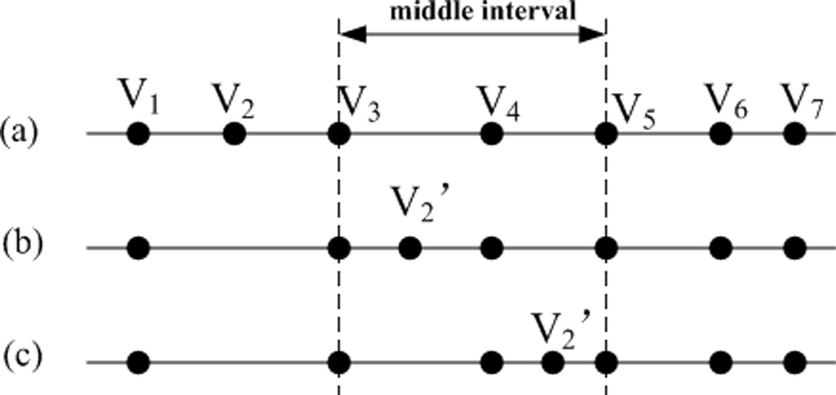

Table 1 show that we divide the changes of the sampled interval into 9 cases. Cases 1, 5 and 9 indicate that there is no change of the sampled interval, so the influence coefficient is 0. Here we take Case 2 as an example. In Case 2, the sample data from the left interval is changed to the middle interval. The data can be dropped before MValue or after MValue.

Figure 1a represents the original sampling situation. We can see that $V_{4}$ is the median and the middle interval is $[V_{3},V_{5}]$ . Suppose $V_{2}$ changes from the left interval to the middle interval and $V_{2}$ is before $V_{4}$ , as shown in Fig. 1b.

We can see that the median does not actually change, and the result is still $V_{4}$ . Because there is an extra node in the middle area, If we directly calculate the median of the data in the filter $M P l a c e$ will offset 1/2 from the $V_{4}$ to the left. So the influence coefficient should be 1/2.

Suppose $V_{2}$ changes from the left interval to the middle interval and $V_{2}^{\prime}$ is after $V_{4}$ , as shown in Fig. 1c. We can see that the median should be $V_{2}^{\prime}$ . If we directly calculate the median of the data in the filter MPlace will offset 1/2 from the $V_{4}$ to the right. So the influence coefficient should also be 1/2. Other things are similar and we don’t prove it one by one.

Because Median query is only a special case of Quantile queries, HAMA algorithm can be easily extended to the Quantile query processing of Wireless Sensor Networks. The only thing that needs to be changed is to change the calculation of the first step of the Median value in the HAMA algorithm to the calculation of the Quantile value, the Quantile value at this time is recorded as QValue, and the position is recorded as QPlace.

4.3 Setting of the equal height histogram interval

In this section, we consider the setting of the histogram interval. Since energy is an important indicator, we mainly consider the effect of interval setting on the energy consumption of nodes. From the algorithm it is easy to see that the energy consumption of the node is divided into two parts, the energy of building the histogram consumption and the energy consumed in the data acquisition phase.

Intuitively, the smaller the histogram is, the less data it needs to be transmitted during the data acquisition phase. But it will also consume energy to build a histogram per round. The smaller the histogram is, the more energy it takes to build a histogram. So we need to find the balance point.

Assuming that there are $S$ nodes in the sensor network and the equal height histogram has $K$ intervals, there are $S/K$ nodes in each interval. Suppose the available capacity of the node message packet is $M$ .

Using cost1 to represent the cost of establishing a histogram. $\textit{COST1}=\left\lceil{K/M}\right\rceil\ast S$ .

Using COST2 to represent the cost of the data acquisition phase, we need to collect samples of about $S/K$ nodes. $\textit{COST2}=\textit{Cost(S/K)}$ .

The cost of each query is $\textit{COST(HMA)}=\textit{COST1}+\textit{COST2}$ . Intuitively, the thinner the histogram is, the fewer data need to be transmitted in the data acquisition stage; however, it takes energy to construct the histogram in each round. The thicker the histogram is, the more data need to be transmitted in the data acquisition stage, so a balance needs to be found. Experiment 3 analyzed it.

4.4 Update strategy of data acquisition interval in HFMA

In the HFMA algorithm, because we do not set up histogram each round, we directly collect the data that falls in the filter $[F_{\textit{low}},F_{\textit{high}}]$ . When the Median value in a new round falls outside the filter, MValue can’t be calculated. Suppose the number of nodes falling in the filter is $M$ , when $\textit{MPlace}<1$ or $\textit{MPlace}>M$ the HFMA algorithm fails.

When the HFMA algorithm fails, we need some additional information to be able to complete the Median query, so we have adopted a new method of sending a new query.

If $\textit{MPlace}<1$ , send the following query.

$\displaystyle\textit{selectTop}(M-\textit{MPlace})$ FromSensors $\displaystyle\textit{Wheresample}<F_{\textit{low}}$

If $\textit{MPlace}>M$ , send the following query.

$\displaystyle\textit{selectBottom}(\textit{MPlace}-M)$ FromSensors $\displaystyle\textit{Wheresample}>F_{\textit{high}}$

Based on time correlation, the median will not be too far away. The data that the query needs to collect will be very small. But as time goes on, the deviation may be getting farther and farther, and the filter should be considered when the deviation is too far away. The adjustment does not need to collect global data, because when MValue jumps out the filter, the query has been sent down to calculate the MValue. We already have data on one side of the MPlace centric interval, and then we can restructure a MPlace centric interval by collecting the other half of the data.

If $\textit{MValue}<F_{\textit{low}}$ in the current round, send the following query.

$\displaystyle\textit{selectTop}\left({\displaystyle\frac{M}{2}}\right)$ FromSensors $\displaystyle\textit{Wheresample}<\textit{MValue}$

If $\textit{MValue}>F_{\textit{high}}$ in the current round, send the following query.

$\displaystyle\textit{selectBottom}\left({\displaystyle\frac{M}{2}}\right)$ FromSensors $\displaystyle\textit{Wheresample}>\textit{MValue}$

5. Experiments

In this section, we evaluate the HMA algorithm and the HFMA algorithm. Sampling and communication are the two main factors that determine energy consumption. Since all algorithms need to sample data, we mainly consider the cost of communication. We use the following two indicators to measure the cost of communication, the average number of packets per round and the lifetime of the network.

Average per round number of packets: the number of network packets within the average per query cycle.

Network lifetime: The network lifetime refers to the number of rounds running from the network to the failure of the node. The nodes near the base station need to transmit more data, so the energy consumption will be faster and it will fail earlier. So, from the view of the availability of sensor network, the network lifetime is a more useful indicator than the total energy consumption.

Table 2
Setting of experimental parameters

Experimental parameters	Value
Number of nodes	961
Area size	100 m*100 m
Communication radius	10 m
Size of message packet	29 byte
Interval of histogram	11
Query running cycle	1000 rounds

Our experiment is designed by OMNet $++$ . Nine hundred and sixty one nodes are distributed in the rectangular area of 100 m*100 m. The communication radius of the node is 10 m, the size of the message packet is 29 byte, the interval of the histogram is set to 11, and the query running cycle is 1000 rounds. Of course, the size of the histogram will have an impact on the performance of HMA and HFMA algorithms. Experiment 3 analyzed it. The node topology is shown as Fig. 2 including 49 nodes. The above is the default setting. If no special description is given, the experiments are used above.

Figure 2.

Network topology.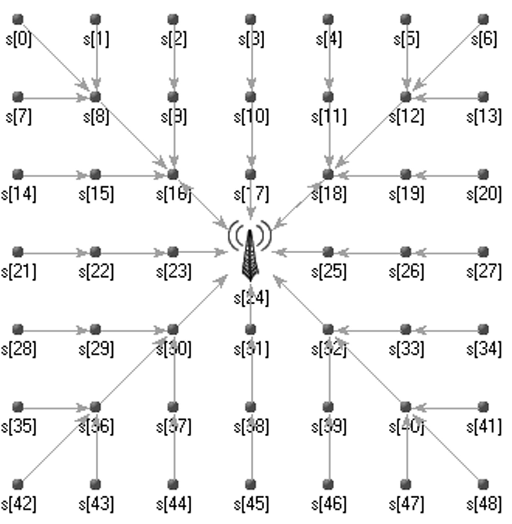

The experimental data contains 2 data sets generated by analog data and real data. We use sensor nodes to sample the temperature and illumination in different campus environment, and obtain the temperature and illumination change model in one day. The initial values of nodes in data set 1 and data set 2 are randomly generated. Sampling of nodes in data set 1 conforming to illuminance change model. The node sampling in data set 2 conforms to the temperature change model.

Figure 3.

The average number of packets per round.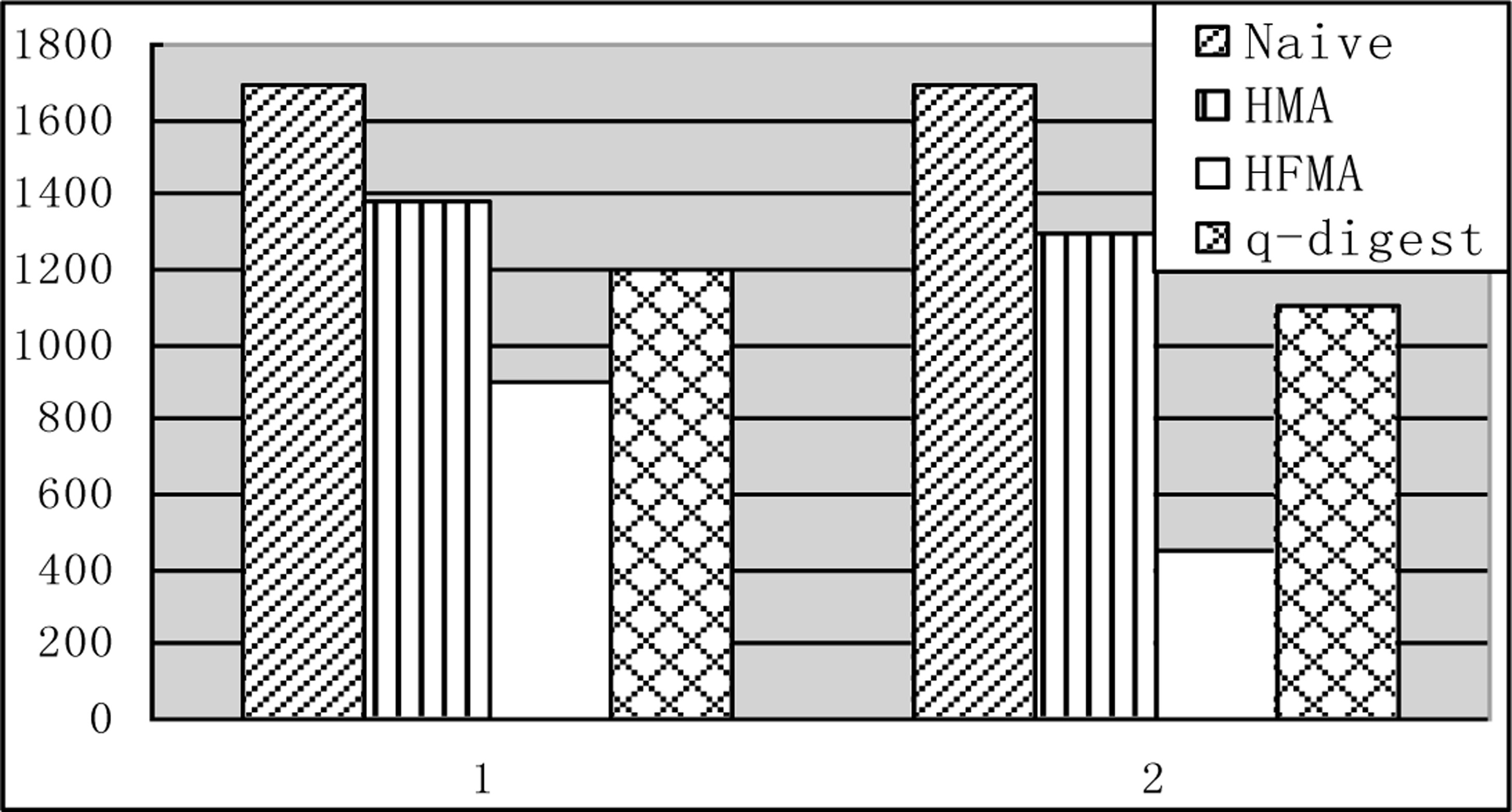

In Experiment 1, we compared the average number of packets per round of Naive, HMA and HFMA algorithms, as shown in Fig. 3. The transverse coordinates indicate the data set used in the algorithm, the longitudinal coordinates represents the number of packets. It can be seen from the graph that the Naive algorithm consumes the most energy, the HMA algorithm is the second, and the HFMA algorithm is the least. Because the Naive algorithm needs to collect the sampling data of all nodes, it consumes the most energy. The HMA algorithm only needs to collect data that falls within the interval of the middle histogram. Compared with the Naive algorithm, there will be a lot less sampling data. But since each round needs to set up a histogram first, it will consume a part of the energy, and in general it reduces energy consumption by about 20% comparing to the Naive algorithm. The HFMA algorithm has better performance than the HMA algorithm because it does not have to set up a histogram in every round.

In addition, we also find that for two different data sets, the performance of Naive algorithm is unchanged, because Naive algorithm always collects data of all nodes. The performance of the HMA algorithm does not change too much, because the cost of building a histogram is the same, and the number of data needed to be collected is roughly the same. The performance changes of the HFMA algorithm are relatively large. The performance in data set 2 is obviously better than in data set 1. We found that the number of effective rounds in the filter will be much more due to the smaller trend of temperature change. The change trend of the illuminance is larger, which leads to the increase of the frequency of the adjustment of the filter, so it will consume more energy.

Figure 4.

Network lifetime.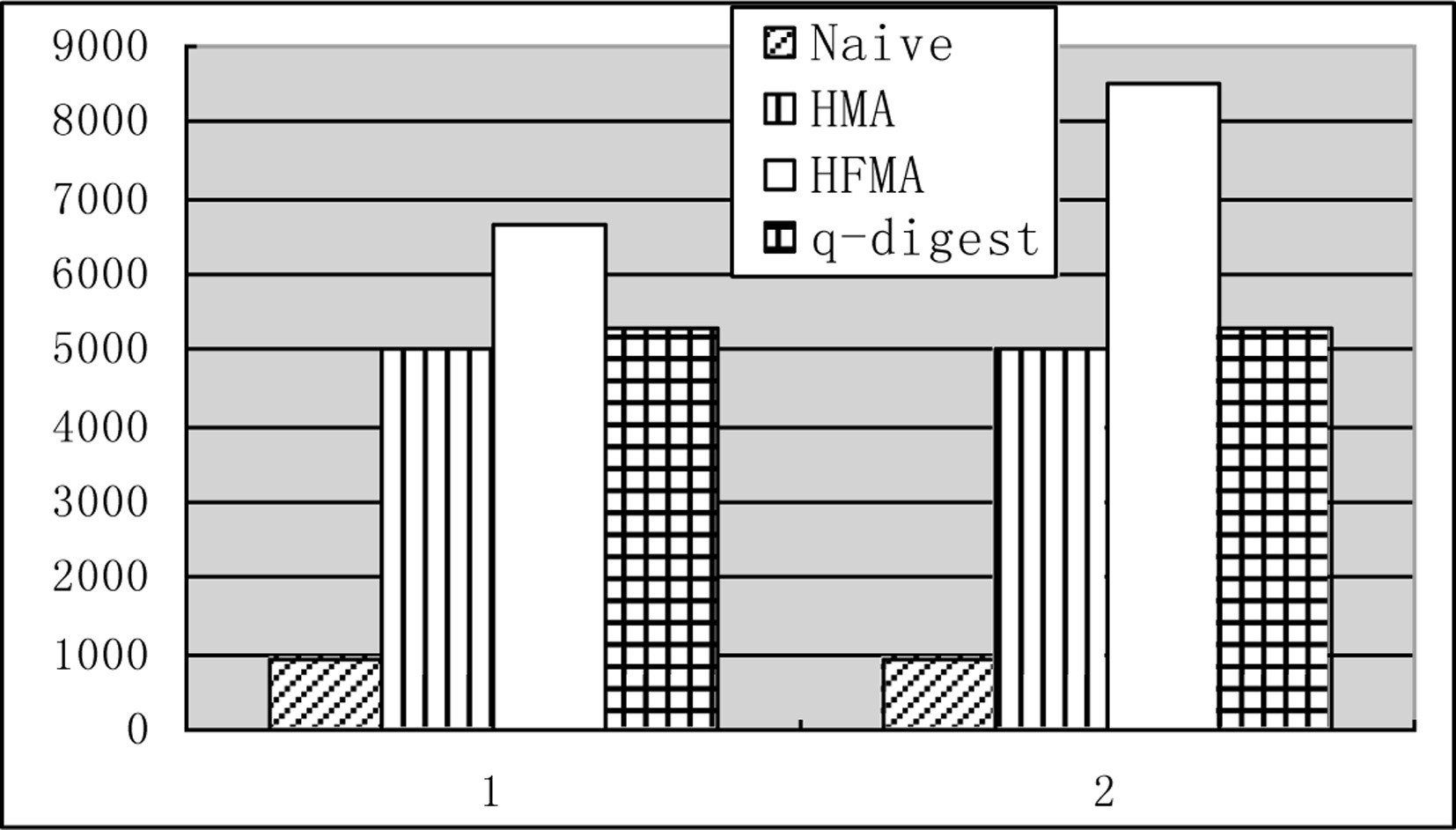

Experiment 2 compares the network lifetime of three algorithms, as shown in Fig. 4. The transverse coordinates indicate the data set used in the algorithm, the longitudinal coordinates represents the network lifetime. As we can see clearly from the diagram, the lifetime of the Naive algorithm is the shortest, the HMA is better, and the HFMA has the longest lifetime.

The lifetime of the HMA algorithm can reach 5 times that of Naive algorithm. For the Naive algorithm, the nodes near the base station need to transmit the sampled data of all nodes on the sub tree, so the energy consumption will be very fast. When it fails, the network lifetime will end. The first stage of the HMA algorithm is to establish global histogram. In the second stage, the data we need to collect has been greatly reduced, so the burden on the nodes near the base station will be reduced a lot, thus improving the lifetime of the network. HMA and HFMA algorithm are more balanced in energy consumption, so there is a longer network lifetime.

Figure 5.

The influence of interval numbers.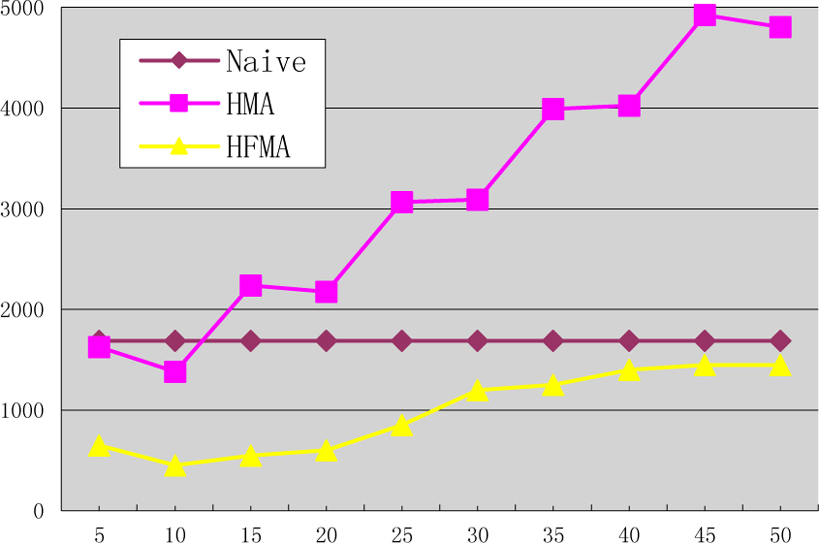

Experiment 3 compares the algorithm performance under different histogram intervals. As can be seen from the graph, the average number of packets in the HMA algorithm increases with the increase of the histogram interval. This is due to the limited capacity of the message packet. When the number of the histogram increases, the energy consumption of the global histogram is also greatly increased.

Of course, the number of intervals is not as small as possible, it can be seen from the figure the algorithm performance, when the interval is 10 are better than the performance when the interval is 5. Because small intervals indicate that more data need be collected.

HFMA achieves best effect when the interval number is 10. When the intervals continue to increase, data packets are on the increase. Less data will fall in the filter when the interval number increased, but the speed of the filter failure has accelerated, frequent adjustment of filter lead to waste more energy.

6. Summary

This paper has studied continuous, accurate median query in Wireless Sensor Networks. First, we propose a median query algorithm based on equal height histogram HMA. Then we extend it and propose HFMA algorithm which combines histogram and filter. In every sampling period, we only need to collect the data that falls in the filter and aggregate the influence coefficient of the data. The base station calculates the median according to the aggregated value of the collected data and influence coefficient. The experiment shows that the HFMA algorithm can effectively save the energy cost and improve the life cycle of the network.

Footnotes

Acknowledgments

The authors acknowledge the Hubei Ministry of Education Foundation (grant: B2016176), Discipline Groups Construction Foundation of Mechatronics and Automobiles of Hubei University of Arts and Science.

References

Kahn

J.M.

Katz

R.H.

and Pister

K.S.J.

, Next century challenges: Mobile networking for Smart Dust, in: Proceedings of the Fifth Annual International Conference on Mobile Computing and Networks, New York: ACM Press, (1999), 271–278.

J.Z.

J.B.

and Shi

S.F.

, Concepts, issues and advance of sensor networks and data management of sensor networks, Journal of Software 14(10) (2003), 1717–1727.

Madden

Franklin

M.J.

Hellerstein

J.M.

and Hong

, Tinydb: An acquisitional query processing system for sensor networks, in: Proceedings of ACM TODS, New York: ACM Press, 2005, pp. 122–173.

Demers

Gehrke

Rajaraman

Trigoni

and Yao

, The cougar project: A work-in-progress report, ACM SIGMOD Record 32(4) (2003), 53–59.

Kang

, In-network processing of joins in wireless sensor networks, Sensors (Basel, Switzerland) 13(3) (2013), 3358–3393.

Branch

J.W.

Szymanski

B.K.

Giannella

Wolff

and Kargupta

, Innetwork outlier detection in wireless sensor networks, in Proc. of ICDCS, 2006, pp. 51–81.

Roh

Y.J.

Song

Jeon

J.H.

Woo

K.G.

and Kim

M.H.

, Energy-efficient two-dimensional skyline query processing in wireless sensor networks, in: Proceedings of the 2013 IEEE Consumer Communications and Networking Conference (CCNC), Las Vegas, NV, USA, 11–14 January 2013, pp. 294–301.

Son

Stehn

Knauer

and Ahn

, Top-k manhattan spatial skyline queries, in: Algorithms and Computation; Springer International Publishing: Cham, Switzerland, 2014, pp. 22–33.

Xin

J.C.

Wang

G.R.

and Zhang

X.Y.

, Energy-efficient SKYLINE queries over sensor network using mapped SKYLINE filters, in: APWeb/WAIM 2007, pp. 144–156.

10.

C.P.

Cong

Tung

K.H.

and Wang

, Incremental maintenance of quotient cube for median, in: Proceedings of the Tenth Acm Sigkdd International Conference on Knowledge Discovery and Data Mining, New York: ACM Press, 2004, pp. 226–235.

11.

Shrivastava

Buragohain

Agrawal

and Suri

, MEDIANs and beyond: New aggregation techniques for sensor networks, in: Proceedings of the 2nd International Conference on Embedded Networked Sensor Systems, New York: ACM Press, 2004, pp. 239–249.

12.

Roy

Conti

Setia

and Jajodia

, Securely computing an approximate median in wireless sensor networks, in: Proc SecureComm, 2008, pp. 1–12.

13.

Hussain

M.M.

Wongse-ammat

and Trajcevski

, Demo: Distributed maxrs in wireless sensor networks, in: Proceedings of the 13th ACM Conference on Embedded Networked Sensor Systems, SenSys’15, pp. 479–480.

14.

Wonge-ammat

Hussain

Trajcevski

, et al., Distributed in-network processing of k-maxrs in wireless sensor networks, Proceedings of the 6th International Conference on Sensor Networks (SENSORNETS 2017), Porto, Portugal, 19–21 February 2017.

15.

Guo

Xiao

, et al., Energy-efficient big data storage and retrieval for wireless sensor networks with nonuniform node distribution, Concurrency and Computation: Practice and Experience 27(18) (2015), 5765–5779.

16.

Madden

S.R.

Franklin

M.J.

Hellerstein

J.M.

and Hong

, TAG: A tiny aggregation service for ad-hoc sensor networks, in: Proceedings of the ACM Symposium on Operating System Design and Implementation, New York. ACM Press, 2002, pp. 131–146.

Filter based continuous median query algorithm in sensor network

Abstract

Keywords

1. Introduction

2. Related work

3. System model and problem definition

3.1 System model

3.2 Problem definition

4. HMA algorithm and HFMA algorithm

4.1 HMA Algorithm

4.2 HFMA algorithm

Table 1 Computing method of influence coefficient

4.4 Update strategy of data acquisition interval in HFMA

5. Experiments

Table 2 Setting of experimental parameters

Footnotes

Acknowledgments

References

Table 1
Computing method of influence coefficient

Table 2
Setting of experimental parameters