1) The problem this paper is going to solve is how to determine the optimal number of dimension when using dimensionality reduction methods, and in this paper, we mainly use local linear embedding (LLE) method as example. 2) The solution proposed is on the condition of the parameter in LLE is set in advance. Firstly, we select the parameter , and compute the distance matrix of each feature in the source data and in the data after dimensionality reduction. Then, we use the Log-Euclidean metric to compute the divergence of the distance matrix between the features in the original data and in the low-dimensional data. Finally, the optimal low dimension is determined by the minimum Log-Euclidean metric. 3) The performances are verified by a public dataset and a handwritten digit dataset experiments and the results show that the dimension found by the method is better than other dimension number when classifying the dataset.
Nowadays, with the development of big data and artificial intelligence, the dimension of data is getting higher and the “curse of dimensionality” causes more difficulties for analyzing the datasets [1]. Dimensionality reduction is often adopted to relieve the critical problem, which can produce the low-dimensional data to represent the original high-dimensional data [2]. The dimensionality reduction methods are divided into linear and nonlinear. Linear methods are mainly principal component analysis (PCA), linear discriminant analysis (LDA) and so on [3], while nonlinear ones are mainly kernel PCA (KPCA) and manifold learning. Linear methods require the data features are independent and the whole data exists in a linear space. Obviously, these requirements limit the usefulness. While, KPCA introduces kernel method into PCA and makes PCA capable of performing complex nonlinear projections for dimensionality reduction [4]. However, the application of KPCA is highly restricted by the fact that there is no definitive way to choose kernel function. Manifold learning can extract the interaction effect and constraint relationship within data and maintain the structural information after dimensionality reduction. Studies have shown that manifold learning has a more proper dimensionality reduction performance on nonlinear data [5].
LLE is one typical method of manifold learning [6]. The essence of LLE is to construct a local linear plane using the sample vector and its nearest neighbor vectors. The sample vector can be linearly reconstructed by its neighbors, and the reconstruction weights minimize the linear reconstruction error between the sample vector and the neighborhood vectors. First, LLE needs to find the first nearest neighbors of sample vectors. Afterwards, it establishes the reconstruction weights embedding into dimension space. Therefore, there are two parameters: number of neighbors and low-dimension [7]. The value of is often chosen empirically, while -dimensional data lies on the nonlinear low-dimension manifold, which is embedded into the high-dimension space. -dimensional data represents the structural feature of manifold. If the dimension is reduced to a low value, the original information will be lost too much. While, if the dimension is still very high after reduction, the redundancy problem may still exist. Though there are many dimension reduction methods, they seldom discuss the determination of the number of low-dimension. In [8], the authors project the face images into two dimensions without giving any specific reasons. In Ref [9], the authors just set the low-dimension as 30,40 and 50 by human experiences. In Ref [10], the authors choose nine methods to reduce face images, regarding the dimension of the highest recognition rate as the best one. In ISOMAP [11] and LLE, the authors only show the variations of facial pose changes by reducing the dimension to be 2. Refs [12, 13] demonstrate that the recognition rate is different when dimensionality is reduced to different dimensions. Therefore, to choose the low dimension in the process of dimensionality reduction is a problem to be solved. Some related works are as follows.
In Ref [1], the authors state that there are two methods to get the estimated intrinsic dimension, which are projection techniques and geometric approaches. Projection techniques, mostly using feature mapping, is a method based on global PCA or local PCA, where the intrinsic dimension is determined by judging whether the number of the ratio of eigenvalues is greater than a threshold parameter. It means a threshold parameter is needed and has a great influence on the final result. On the other hand, geometric approaches use the correlation dimension to estimate the intrinsic dimension, and require the number of samples to be infinity at best, but in practice there are just finite sample vectors. In addition, Ref [11] calculates the correlation coefficient between the distance matrix of the high-dimensional data and low-dimensional data in order to obtain residual variance. Using the trend of the residual variation to find the elbow vector to be the intrinsic dimension, but the trend is not easy to locate the elbow vector. Ref [14] indicates that fractal methods require a -dimensional ball of radius and count the number of vectors which is a neighborhood of radius , but the condition requires the number of samples to be exponentially increasing if the dimension increases in order to obtain an accurate estimation. Ref [15] presents that maximum likelihood estimation methods [16] will give different low dimension results if the nearest neighbor number varies. In Ref [17], the authors propose to use -nearest neighbor graphs to establish the sum of distances between sample vectors and neighbors, and construct an approximation function to estimate the eigenvalues, and in Ref [18], the authors consider the structure and spectral information for selecting effective spatial-spectral neighbors of hyperspectral image pixels and explores the spatial relationship between each point and its neighbors to do dimension reduction, and in Ref [19], the authors propose a low-dimension estimator using only the distance of the first and the second nearest neighbor of each point in the sample and it is able to reduce the effects of curvature, of density variation, and the resulting computational cost, but all of them do not discuss the way to choose the number of low-dimension.
In this paper, we propose a solution to compute the optimal low dimension. First, we find nearest neighbor vectors of each sample vector, then find the graph relationship between the sample vector and its nearest neighbor vectors. We use Dijkstra algorithm to locate and determine the shortest path from the sample vector to each vector, and compute the distance matrix of each feature and low-dimension data. Next, we compute the metrics value between distance matrix of every feature and the distance matrix of low-dimension data by Log-Euclidean Metric. Distance matrix metrics can represent the distance relationship between high-dimension data and low-dimensional data. When the metrical values are small, it means that the information loss caused by dimensionality reduction is very low. Therefore, we choose the -dimension corresponding to the minimum metrics as the optimal dimension.
The main contributions of this paper are in the following:
The paper proposed a kind of solution to find the optimal number of low dimension for dimension reduction algorithms, specifically for LLE method adopted in the paper.
The paper gave a comparison experiment to verify that the dimension found by the proposed method can improve the classification accuracy for different dimension reduction algorithms.
This paper is organized as follows. In Section 2, the paper overviews the process of using LLE algorithm. Section 3 gives the main process of the proposed method to find the optimal number of low dimension. In Section 4, the experiments with results are shown. The conclusion is given in Section 5.
Overview of LLE algorithm
The processes of the LLE algorithm are:
To select nearest neighbors of each sample vector:
There are sample vectors, i.e. . We use Euclidean distance computation to determine neighborhood around a sample vector. Choose the number of nearest neighbors: . Imagine is the sample vector, and is its neighbor, and is the weight between and . As such, can be represented by :
To compute the reconstruction cost caused by the approximation of each sample vector and its neighbors, and the reconstruction weights are to be computed in the following:
where denotes the nearest neighbors of . By computing, can be computed by the following formula:
where .
In the process of embedding, the reconstruction weight remains fixed in the low-dimension space, so that each vector in the high-dimensional space corresponds to in the low-dimension space:
By formulating the coefficient matrix, we have . Computing eigenvalues and eigenvectors of matrix , we select the eigenvectors corresponding to the smallest eigenvalues of to be the low-dimension data , where . Further, we use the distance matrix and Log-Euclidean Metric to measure the effect of dimensionality reduction.
Computation of the number of low dimension
Distance matrix between sample vectors based on dijkstra algorithm
First we choose and different value of , then compute the distance matrix as follows:
where means distance matrix when we choose nearest neighbors for the -th feature. In this case, we find a problem: when , we describe all neighbors as a graph structure, but not all pairs of sample vectors are linked directly. It is unreasonable to compute that distance by Eq. (5). To solve this problem, we use Dijkstra algorithm to compute the sample pairs without directly connection. Dijkstra algorithm will determine a “source” node, which is a single node, and will choose the paths with the shortest length from the source node to the other nodes in the graph [20]. We can use it to compute the distance matrices , and do the same for the low-dimension data. For the low-dimension data, the following distance matrices formula is adopted:
where is the number of the nearest neighbors and the number of the low dimension is . As for computing matrix metrics between feature distance matrix, that is and feature distance matrix, that is , the paper adopts the Log-Euclidean Metric.
Log-euclidean metric
Log-Euclidean Metric can measure the distance between two matrices [21, 22]. It is flexible to compute and commonly used as a tool in computer science field.
Performing the diagonalization for , to obtain a matrix which is called the rotation matrix and a matrix with the eigenvalues of to be its diagonal elements. The equality holds: ;
Transforming all the diagonal elements within the matrix into their logarithm computation results, in order to procure a new diagonal matrix ;
Re-compose and to have the final logarithm computation results with the following equation
Compute the distance metrics via the following rule
For instance, we set three matrices :
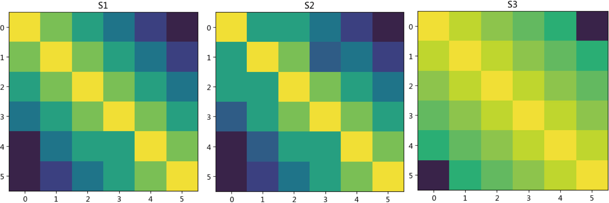
We draw the heat maps of in which the larger the value is, the lighter the color while the smaller the value is, the darker the color. We can see from the Fig. 1, that the color of and are similar, but the color of and are not. We use Log-Euclidean metric to compute and get the results in the following:
Heat maps of .
We can see the metrics between and is small, so the distance between and can be determined to be close. By this example, we can affirm that using Log-Euclidean metric to measure the distance between matrices is sound.
Selection of the optimal value of low-dimension
Compute the Log-Euclidean metric between each feature distance matrix and low-dimensional data distance matrix . After measuring all the features in sample vectors and low-dimension data, we sum the results and regard the sum as the relation metrics of and as follows:
where is the number of nearest neighbors, is the low dimension, is the original value of dimension, is the -th feature distance matrix, is the low-dimension data distance matrix, and is the metric cost with nearest neighbors and low dimension.
By iteration, we choose different value of low dimension as to get the corresponding metric cost of each chosen low dimension. Meanwhile, the number of nearest neighbors needs to be changed. Comparing all those iterative results, we select the minimum as the result:
where is just the optimal low-dimension value with nearest neighbors.
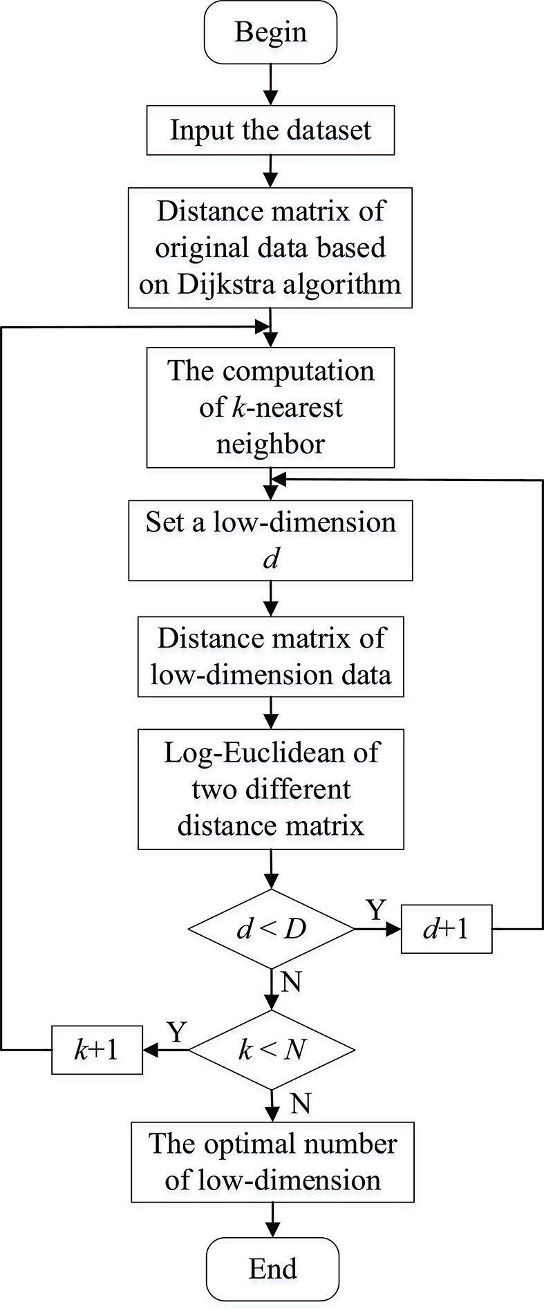
The flow chart of the proposed method is in the following:
Flow chart of the proposed method.
Experiments
Wine dataset
We use one public classic dataset from UCI, that is wine dataset, as experimental data. It has 178 samples with 13 dimensions.
Experiment procedure
In this experiment, we choose 15, i.e. . Low-dimensional data is . In the process of dimension reduction, we need choose two parameters: the number of nearest neighbors and the number of low dimension .
When , , we get three nearest neighbors of each sample vector, and draw the graph to compute the distance matrix of each feature;
Compute the low-dimension data, and get the distance matrix of low-dimension data, i.e., ;
Compute the distance metrics between distance matrix of each feature and low-dimension data, to get the metrics value, i.e., ;
Choose different number of , and get the distance value , by comparing those results to choose the with the minimum value as the best one;
Choose different number of , and obtain the minimum metric cost.
In Table 1, we show the neighbor sample results for wine dataset. For the chosen 15 samples, we give each sample the corresponding neighbor sample index.
The number of the neighbors for each sample vector with ,
Source
First neighbor
Second neighbor
Third neighbor
0
1
9
8
1
8
9
0
2
13
11
6
3
5
10
12
4
9
8
1
5
3
10
12
6
11
7
12
7
6
11
12
8
9
0
1
9
8
1
0
10
3
5
12
11
6
7
12
12
6
11
7
13
2
0
1
14
10
3
5
Experimental results
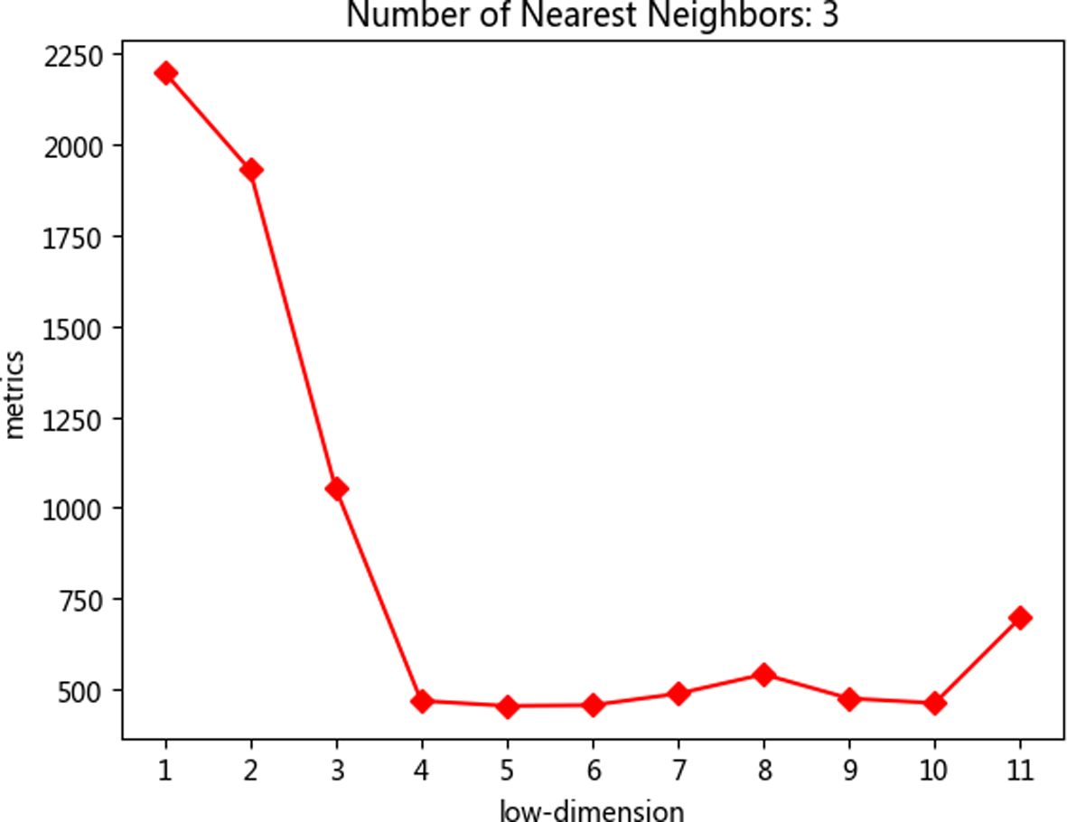
When , we get the metrics values for different low dimension, as shown in Table 2 and Fig. 3.
Metrics of different low dimension with
Low dim
1
2
3
4
5
6
7
8
9
10
11
Metric cost
2200.2
1930.7
1053.99
467.69
453.54
455.56
487.32
540.53
474.12
461.38
696.48
The metric costs of different when .
The metric costs of different and
Low dim
1
2
3
4
5
6
7
8
9
10
11
4
86.37
80.13
80.78
73.25
70.73
76.69
78.31
75.99
76.35
76.19
78.46
5
91.51
84.38
79.33
84.21
75.02
79.54
78.81
78.83
79.44
83.37
78.74
6
89.11
92.24
85.16
84.33
89.46
86.25
85.38
84.63
84.51
84.54
84.95
7
89.36
103.04
88.94
88.99
88.85
87.87
89.00
88.96
88.93
91.99
89.30
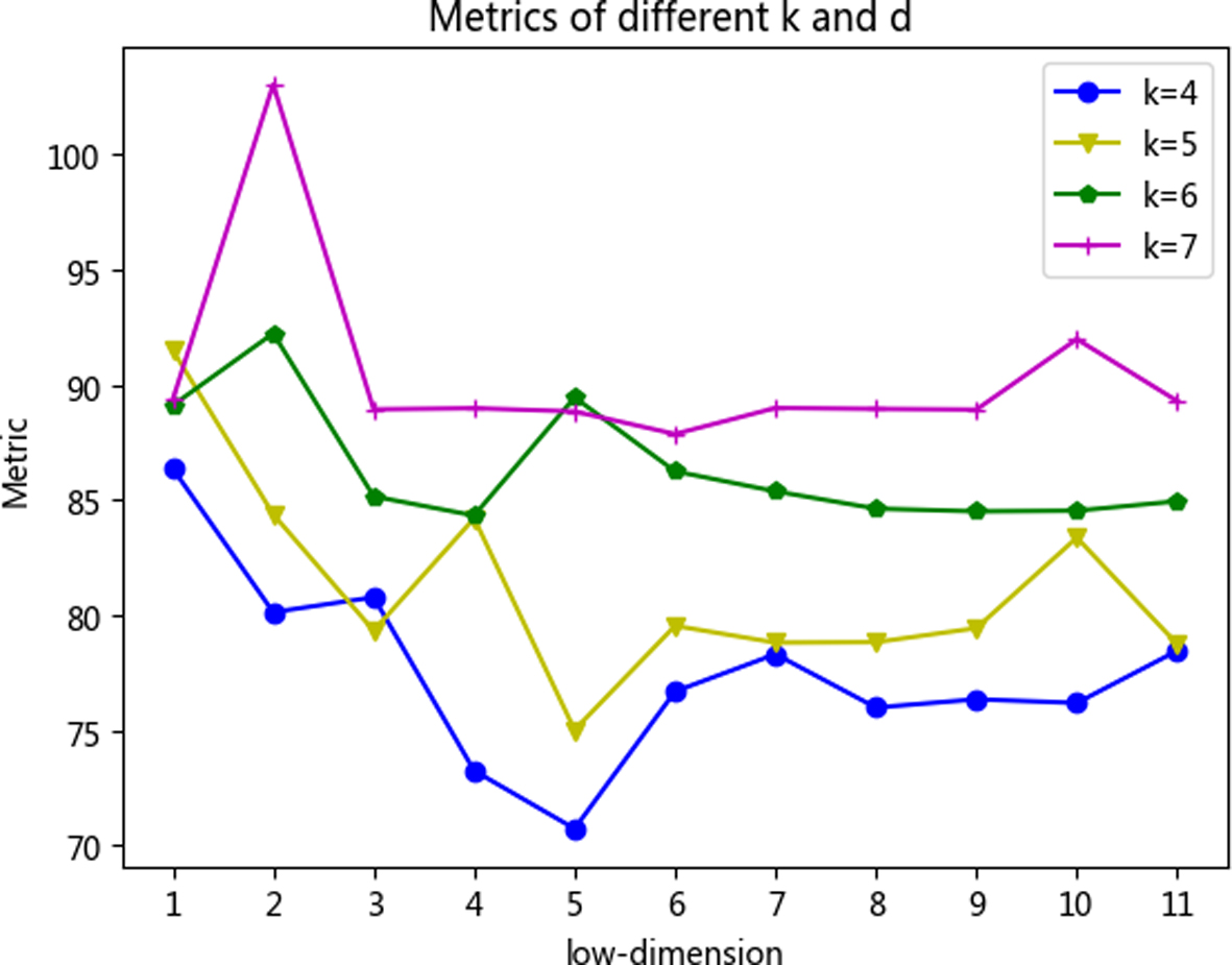
Metric costs of different and .
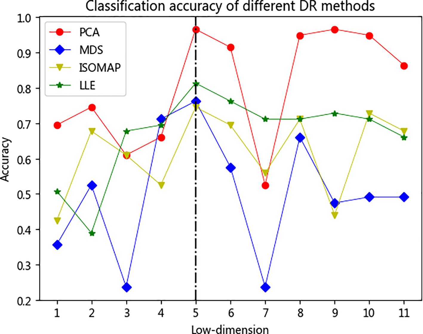
The classification accuracy after different dimension reduction methods.
From Fig. 3 and Table 2, we can see that when choosing 3 neighbors, the trend of the metric costs decline before dimension 5. When , we get the minimum metrics. After that, the metrics begin to rise and get the local maximum when and then decline again. In the whole process, we always have the minimum metrics when ; therefore, we let the optimal number of low dimension be 5.
When different number of is chosen and the number of neighbors is gradually increased from 4 to 7, the result are as follows:
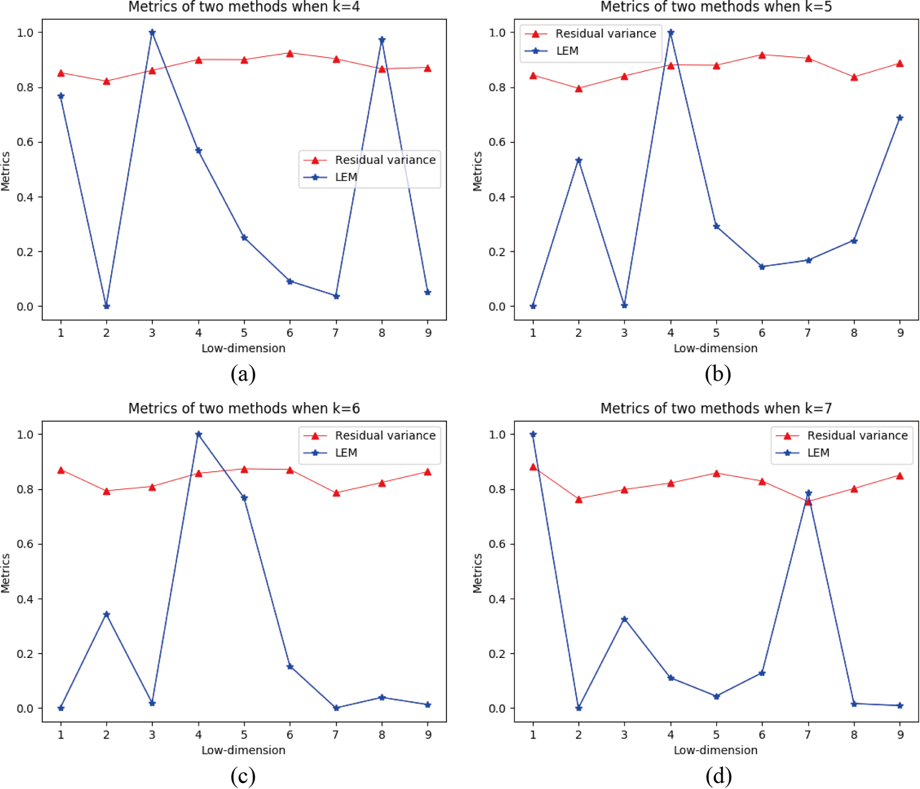
We use the line graph to draw the metrics for each dimension when the number of neighbors is varied from 4 to 7. As shown in Fig. 4, the optimal low-dimension of the wine dataset by LLE method can be determined by combining Fig. 3 and Table 3. The conclusion is that dimension is 5 with the number of neighbors to be 4.
Metric costs of the two methods with different and .
In order to show that the optimal low-dimension is efficient, we also use PCA, MDS, ISOMAP and LLE methods to reduce the dataset dimension to be for wine dataset. There are three class labels in the wine data set. We choose two thirds of dataset for training and the rest for testing. Linear SVM classifier is used to perform the classification prediction and the accuracy is used to judge the efficiency.
From Fig. 5, we can see that using different methods to have the dimension reduction results for the dataset ‘wine’, and when low-dimension is selected to be 5, all the methods can give the highest classification accuracy. Therefore, using our proposed technique to determine the optimal low-dimension is reasonable. It should also be noted that the wine data is not strictly manifold structured dataset, and in the whole, PCA shows higher accuracy than other methods based on manifold.
MNIST handwritten digits data set experiment
For handwritten digits dataset MNIST, we select the ‘5’ and ‘6’ digits in the handwritten number to conduct experiments. Each digit selects 100 images randomly, and each image is converted to a vector with dimension, then we get 200 samples, each of dimension 784.
When to reduce the dimension, we select the number of neighbors to be 4, 5, 6, and 7, and vary the target low dimension from 2 to 9. We compare the method of the residual variance in the literature [11] with our proposed method. The residual variance formula is , in which is the matrix of Euclidean distance in the low-dimensional embedding and is the matrix of Euclidean distance of the original high-dimensional data, while is the standard linear correlation coefficient. The proper low dimension given by residual variance is the elbow vector for the variation of the residual variance.
For the experimental dataset, we draw the proposed metric (LEM) values and the result of the residual variance into a line graph, as shown in Fig. 5, in which all the results are normalized by the proposed metric cost.
From Fig. 6, we can see that using the proposed metric to find the optimal dimension is much more obvious than residual variance. When , the optimal dimension is 2 and when , the optimal dimension is 3 and when , the optimal dimension is 3 while , the optimal dimension is 2. However, using the residual variance method, it is difficult to find an elbow vector in each case. And by this experiment, it is noticed that when the number of neighbor changes, the optimal dimension will also change also; therefore, the neighbour number should be selected properly.
Conclusions
In this paper, we propose a method to search the optimal value of low dimension, when using LLE. First, we select the nearest neighbors of each sample vector to compute the distance pairwise and then use the Dijkstra algorithm to construct the graph and measure distance matrix of each feature and low-dimension data. The metrics between the distance matrix of each feature and low-dimension data by Log-Euclidean metric is computed. Afterwards, we choose the optimal low dimension d with the minimum metrics. In the experiments, the results of the wine dataset from UCI and MNIST handwritten digits dataset show the proposed method can find an optimal low-dimension. By using our method, the information loss caused by dimension reduction is expected to be minimum. The further extension application is to use the proposed method for other dimension reduction algorithms to find the proper low dimension. The limitation of this method is that noises within the data can affect the performance. The further research will consider the effects of the noises in the data samples when to reduce the dimension and find the optimal number of low-dimension.
Footnotes
Acknowledgments
This work is partly supported by the National Key R&D Program of China (2017YFB0702100), National Natural Science Foundation of China (No. 61903029), National Material and Environment Corrosion Platform of S&T of China and project of The Ministry of Education, Youth and Sports of the Czech Republic (No. 8JCH1067).
References
1.
KéglB., Intrinsic dimension estimation using packing numbers, Advances in Neural Information Processing Systems (2003), 697–704.
2.
CunninghamJ. and ByronM., Dimensionality reduction for large-scale neural recordings, Nature Neuroscience17 (2014), 1500–1509.
3.
CunninghamJ. and GhahramaniZ., Linear dimensionality reduction: Survey, insights, and generalizations, Journal of Machine Learning Research16 (2015), 2859–2900.
4.
ZhenxueH.GuicangZ.JunQ. and LinyingY., Symmetric kernel principal component analysis and its application in face recognition, Computer Engineering39 (2013), 174–173.
5.
WangQ.WangW. and NianR., Manifold learning in local tangent space via extreme learning machine, Neurocomputing174 (2016), 18–30.
6.
RoweisS.T. and SaulL.K., Nonlinear dimensionality reduction by locally linear embedding, Science290 (2000), 2323–2326.
7.
LiuY.ZhangY. and YuZ., Incremental supervised locally linear embedding for machinery fault diagnosis, Engineering Applications of Artificial Intelligence50 (2016), 60–70.
8.
VepakommaP. and ElgammalA., A fast algorithm for manifold learning by posing it as a symmetric diagonally dominant linear system, Applied and Computational Harmonic Analysis40 (2016), 622–628.
9.
FanM.ZhangX. and QiaoH., Efficient isometric multi-manifold learning based on the self-organizing method, Information Sciences345 (2016), 325–339.
10.
WangG.ShiN. and ShuY., Embedded manifold-based kernel Fisher discriminant analysis for face recognition, Neural Processing Letters43 (2016), 1–16.
11.
TenenbaumJ.B.SilvaV. and LangfordJ.C., A global geometric framework for nonlinear dimensionality reduction, Science290 (2000), 2319–2323.
12.
WangJ.ZhangB.QiM. et al., Linear discriminant projection embedding based on patches alignment, Image and Vision Computing28 (2010), 1624–1636.
13.
AbazaA.RossA.HebertC. et al., A survey on ear biometrics, ACM Computing Surveys45 (2013), 1–35.
14.
FaccoE.D’ErricoM.RodriguezA. et al., Estimating the intrinsic dimension of datasets by a minimal neighborhood information, Scientific Reports7 (2017), 12140–12145.
15.
GolayJ. and KanevskiM., A new estimator of intrinsic dimension based on the multipoint Morisita index, Pattern Recognition48 (2015), 4070–4081.
16.
MoD. and HuangS., Fractal-based intrinsic dimension estimation and its application in dimensionality reduction, IEEE Transactions on Knowledge & Data Engineering24 (2011), 59–71.
17.
KpotufeS., KNN regression adapts to local intrinsic dimension, Advances in Neural Information Processing Systems1 (2011), 729–737.
18.
HongH.GuangyaoS.HaiboH.YuleD. and FulinL., Dimensionality reduction of hyperspectral imagery based on spatial-spectral manifold learning, IEEE Transactions on Cybernetics (2019), 1–13.
19.
ElenaF.MariaE.AlexR. and AlessandroL., Estimating the intrinsic dimension of datasets by a minimal neighborhood information, Scientific Reports12140 (2017), 1–8.
20.
QingG.ZhengZ. and YueX., Path-planning of automated guided vehicle based on improved Dijkstra algorithm, Control and Decision Conference (2017), 7138–7143.
21.
ArsignyV.FillardP.PennecX. et al., Log-Euclidean metrics for fast and simple calculus on diffusion tensors, Magnetic Resonance in Medicine56 (2006), 411–421.
22.
HuangZ.WangR. et al., Log-Euclidean metric learning on symmetric positive definite manifold with application to image set classification, Int Conference on Machine Learning37 (2015), 720–729.