Statistical approach to compute a surrogate input for building physics CFD simulations through experimental measurements

Abstract

Computational Fluid Dynamics (CFD) simulations are sensitive to input uncertainties and human errors. Using real-world data as an input for CFD simulations is not rare for building physics simulations and it is still an open topic. In most cases, computer simulations using CFD are for design purposes and they aim to represent the situations occur in the real-world. The real-world parameters are commonly set based on experimental measurements. However, it is known that experimental measurements are affected by uncertainties; hence the experimental values have to be processed to calibrate numerical simulations. This paper investigates the CFD simulation calibration through experimental measurements. In particular, a statistical approach is employed to study the experimental data of inlet-outlet velocities for ten non successive days in a test-room with the purpose of assuming a surrogate day input that is the most significant of the dataset. Moreover, five different input methods on the boundary conditions of inlet velocity obtained from the experimental measurements are implemented and the accuracy of the predicted results through CFD simulations is presented. For the first input, the actual measurements of one particular day were chosen among the ten available days. For the other four, the numerical input relating to each second of the synthetic day was constructed by means of a statistical assessment of the actual measures obtained at each corresponding second of the ten actual days. The Hermite polynomial chaos expansion was selected for the last approach. Results have shown a significant variability of airflow for both experimentally measured input and output signals. By using the experimental signal expansion through Hermite polynomials the experimental and numerical values give satisfactory results.

Keywords

Experimental data statistics Hermite polynomial chaos expansion CFD simulations

1. Introduction

Nowadays, the use of computational simulations is increasing day by day in order to optimize the costs of performing experimental tests. Computational fluid dynamic simulations (CFD) are usually calibrated by experiments [1, 2, 3]. In the field of wind and environmental engineering, experiments are carried out on scaled models in wind tunnel [4] or in the environment [6, 7]. Frequently, experimental tests entail high costs and a long time which results in a reduction of specimen size at the expense of accuracy to reproduce the phenomena. Sometimes CFD simulations are computed without experimental results to compare [8]. In addition, experiments carried out directly in an open environment are usually not so easy to reproduce and vulnerable to possible assessment flaws that may heavily affect the realistic reproduction of phenomena, as in the case of [9]. During several trials, he compared both wind velocities and directions, which were measured simultaneously without any corrections depending on the different height positions of the related instruments [10] discussed the reliability of their CFD simulation by comparing numerical and experimental results. In this case, the authors discussed the experimental setup but they did not give any clarification about the comparison. For example, they did not clarify whether the numerical results were compared with mean or peak experimental results [11] compared CFD results by following a similar approach. In fact, they did not give any information about the experimental signals statistics and the experimental data sample chosen to be compared.

Based on the motivations mentioned above, CFD simulations are calibrated by a restricted database. It is evident that both the selection of the experimental sample and the calibration-validation of the used numerical tool are crucial steps in order to obtain useful outcomes. The first (i.e. selection of the experimental sample) depends on objective factors, for example, the investigated phenomenon and the available instrumentation or the environmental conditions, while the second (i.e. calibration-validation) is often subjective. In fact, the analyses may be carried out by using a single value or a single time history of values that summarizes the experimental data set as input data. It is evident that, in both cases, the resulting selection should be the optimum choice for reproducing the investigated phenomenon.

The variability and uncertainty of the numerical values caused by the selected input data usually affected by a tolerance interval which should be taken into account in the evaluation of the results. This issue is partially discussed in the literature, not only in the CFD framework but also in many other fields. In particular [3], inferred that there is no clear procedure to validate numerical data and quality requirements to be satisfied by validation data [12]. At first, CFD steady-state models require validation data from experiments under steady-state atmospheric conditions, but the atmosphere is fundamentally time-dependent and never in a steady state. In fact, weather conditions are continuously variable and the fluctuations in the incoming wind affect flow stability. Consequently, measurements taken a few meters apart from each other might show largely different results [13].

In most field experiments only one reference station exists, which can be utilized to characterize the meteorological conditions and be used as model input, however, there are some exceptions. For example [14], acquired data using multiple locations in parallel. Observing the experimental data set variability based on the daily atmospherically variations, the purpose of the research executed by [1] was to analyze the dependence of CFD output on the input data statistics regarding a selected test case [15] provided a survey of the role of statistics on the interaction between experimental data and design. In particular, the author discussed the effect of data set in the field of medicine. Similarly [16], discussed the potential pitfalls of inadequate experimental design and provided suggestions for the selection of a suitable statistical test of experimental data. Moreover, in Geomechanics, some authors have been discussing the relations between the impact of the input data variability on the outcomes of numerical simulations [17, 18, 19, 20, 21, 22].

In this paper, experimental data statistics were used to obtain different CFD input data that are used to estimate different CFD output data to make comparisons with experimental values. The purpose was to assume a surrogate input representing the most significant experimental dataset. The goal was replacing the entire experimental database that is used to calibrate CFD simulations with the surrogate input. In order to achieve this, experimental measurements with three anemometric sensors were carried out on a sample case of a prismatic 5.2 $\times$ 3.4 $\times$ 2.7 m room located on the second floor of a building. The first sensor was located outside in the environment. The second sensor was in the inlet, while the third one was in the outlet of the room. The goal was to show the different results obtained by using different velocity time histories in the inlet as input for CFD simulations. The selection was the crucial aspect of this investigation. The measurements were repeated for ten days. For each second, ten time histories were obtained for the environmental wind velocity, inlet wind velocity and outlet wind velocity. However, the CFD simulations were executed to make comparisons between numerical outcomes and the measurement data obtained from one specific day which was considered as a surrogate day and representative of the entire experimental data set. Five different input time histories were explored by processing the experimental data acquired at the inlet measurement points. Details in regard to this are described in the following sections. In order to compare the numerical results obtained through the application of the CFD method, the experimental data related to the outlet flow velocities were re-elaborated according to the surrogate day by applying the same statistics adopted for the respective input time histories.

In this study, only one model was used for CFD simulations. However, systematic studies for a given problem that were performed by several operators who have applied the same model [23], or executed either by a single operator or by several operators who have applied different models [24] have shown significantly different numerical outcomes. The mean percentage error between the experimental inlet and outlet data set and numerically generated CFD input time histories and output results were assumed to be a good measure of precision [25].

2. Methodology

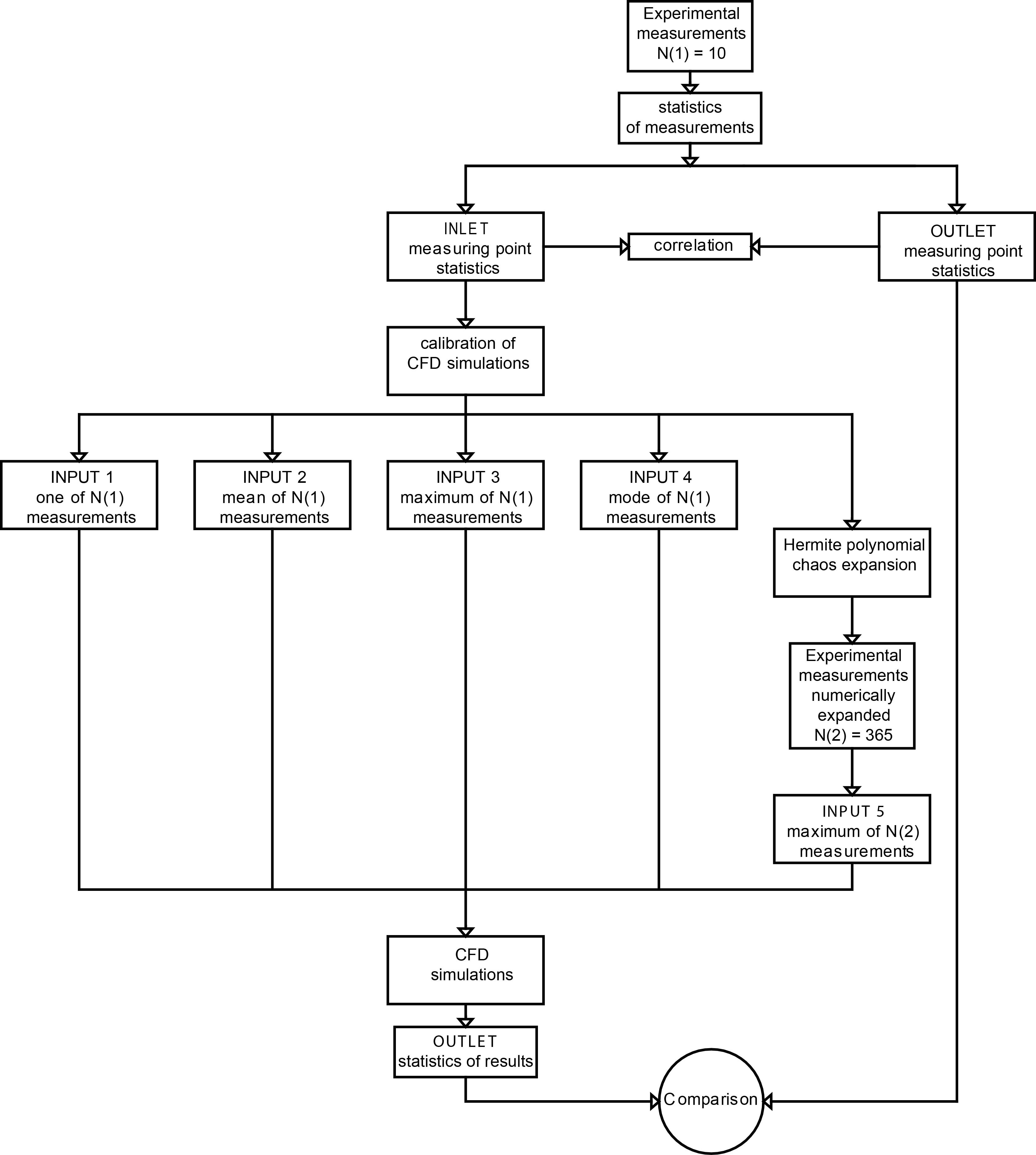
To facilitate the reading of the following sections, an overall step-by-step description of the approach followed in this research is presented in this section and illustrated in Fig. 1. The inlet and outlet air flow velocities are recorded for ten days and subdivided in ten records. All records can be used merged in one signal as inlet input for CFD simulations. However, in the case of several registrations it can require unsustainable time of calculation for the most of researchers.

In order to reduce the computational calculation time, the purpose is to estimate a surrogate input signal, derived from experiments, to perform CFD simulations. The goodness of the surrogate input signals was measured as the agreement between the numerical outlet signal and the measured outlet signal. These agreement was estimated comparing the statistics of the numerically and measured outlet signals and the correlation coefficients between inlet and outlet signals.

The correlation coefficient between inlet and outlet was used as a measure of the undisturbed flow streamlines propagation. In the case of big value of the correlation coefficients was concluded that the flow is undisturbed. It was assumed that a reliable simulation of the experimental tests should give the same good agreement in term of correlation between the inlet and outlet signals.

Figure 1.

Procedure overview.

The search for a surrogate inlet signals was completed examining five different surrogate inlet signals: the first was one inlet measurement, the second was the mean (i.e. second for second) of the ten measurements, the third is the maximum (i.e. second for second) of the ten measurements, the fourth is the mode (i.e. second for second) and finally, the fifth is a signal obtained expanding second for second the ten recorded time steps through Polynomial chaos Expansion [26, 27, 28, 29]. Ten days acquisitions were analytically expanded to one year signals. The fifth surrogate inlet signal was obtained by the maxima second for second of the one year data set.

The Polynomial Chaos Expansion (PCE) is based on a spectral representation of a random variable [30]. This approach is successfully used in the field of civil engineering to estimate the experimental error effects on the structures’ reliability [26, 27, 28, 29]. On a probability space ( $\Theta$ , $\Sigma$ , $P$ ), if one denotes by $\theta$ the random event belonging to the domain $\Theta$ , a generic realization of a random variable, in this case $V_{(1)}$ , can be formally written as $V_{(1)}$ ( $t;\theta$ ) according to Eq. (2):

$\displaystyle V_{\left(1\right)}\left({t;\theta}\right)=\mathop{\sum}\limits_{% j=0}^{P}h_{j}^{\ast}\psi_{j}\left({\xi\left(\theta\right)}\right)$ (1)

In the previous equation, the truncation order of the expansion is denoted by $P$ (degree equals 4 ${}^{\rm th}$ order in this paper); the $\psi_{j}$ quantities are polynomials of degree $j$ used by the expansion; $\xi(\theta)$ is a realization of a seed random variable; the $h_{j}^{\ast}$ is a quantity which is a normalized scalar coefficient of the polynomial chaos expansion that needs to be determined. This representation transforms a seed random variable $\xi(\theta)$ into a more general random variable by a nonlinear translation process [31]. The $\psi_{j}$ polynomials are selected as mutually orthogonal with respect to the probability density function of the seed variable. The seed is usually represented by a standard Gaussian variable recast in terms of normalized Hermite $\psi_{j}$ polynomials (or “Hermite chaos”), as in the original polynomial chaos decomposition [30]. Yet [32], worked on more general distributions.

The representation in Eq. (2) was applied to the distribution of the probabilities of several random variables obtained from experimental data, for example on uncertain stiffness properties of instrumented structures [33] , and on elastic properties of random media [34]. In the field of wind engineering, this representation and the concept of translation process based on the Hermite model were employed to replicate non-Gaussian features of intermittent wind pressure fields [35] and the non-Gaussian extreme values of the response in wind-excited structures [36]. Recently, the PCE and the corresponding spectral methods were explored to study flutter probability caused by the errors in flutter derivatives [37, 38]. This kind of expansion requires the estimation of $h_{j}^{\ast}$ coefficients. In this study, the numerical procedure proposed by [33] was utilized to determine $h_{j}^{\ast}$ .

3. Experimental measurements

3.1 Experimental setup

The experimental setup was equipped to measure the inlet and outlet velocities in a room with the purpose to investigate the induced error on CFD simulations by experimental values. The experimental setup is voluntarily simplified in order to reduce the most common effects, such as the pressure drop and the vortex shedding. It is important to note that the results discussed here represent a part of the research that is focused on the thermal isolation of a room in underground conditions that uses Polystyrene panels to reproduce the environmental conditions.

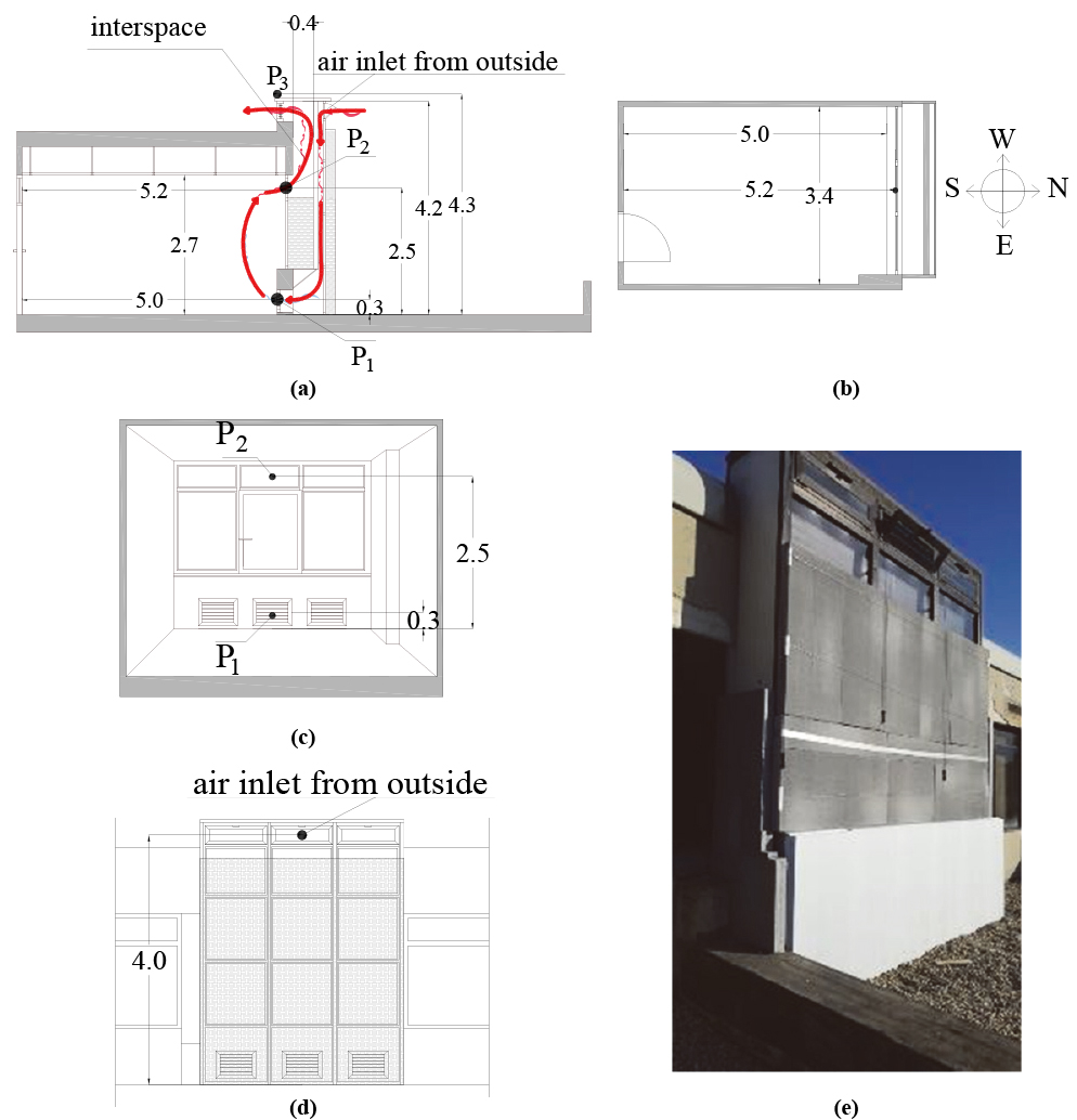
The test room is located at the University G. D’Annunzio building, in Pescara, Central Italy. The room dimensions and geometry are illustrated in Fig. 2 [25]. The room’s dimensions are about 5.0 $\times$ 3.4 $\times$ 2.7 m and it opens outward on the north-western border, while the other borders are adjacent to the other offices. Figure 2a and b show the cross-section and plan view of the room and the positions of outside ( $P_{3}$ ), inlet ( $P_{1}$ ) and outlet ( $P_{2}$ ) sensors. Figure 2c shows an internal perspective view of the room, whereas Fig. 2d shows an external view of the north-western border window. As shown in Fig. 2, in panels a and c, the sensors were located perpendicularly to the vent and to the façade.

Figure 2.

Schematics of the test rig: Schematic drawing of test room cross-section (a), plan view (b), in perspective internal view (c), external view (d) and a picture of the northern border window (e).

Except for the interspace with dimensions of 0.4 m in length and 4.2 m in height, the room is impermeable for airflow. Two ESV-BSV105 60 $\div$ 130 mV hot-wire anemometers (i.e. accuracy 0.1 m/s) were used in inlet ( $P_{1}$ ) and outlet ( $P_{2}$ ), and one DNA021 0 $\div$ 1235.67 Hz hemispherical cup anemometer was used outside ( $P_{3}$ ). In addition, three EST-BST101 $-$ 50 ${}^{\circ}$ C $+$ 80 ${}^{\circ}$ C temperature sensors (i.e. accuracy 0.2 ${}^{\circ}$ C) were coupled with three velocity sensors. All sensors were calibrated in February 2019.

Measurements were carried out for ten full days, from May 4 ${}^{\rm th}$ to May 17 ${}^{\rm th}$ . During the experiments, the outside temperature varied from 18 ${}^{\circ}$ C (i.e. during the night) to 28 ${}^{\circ}$ C (i.e. at noon), with mainly sunny weather without rain. The sampling frequency was assumed to equal to 1 Hz [19].

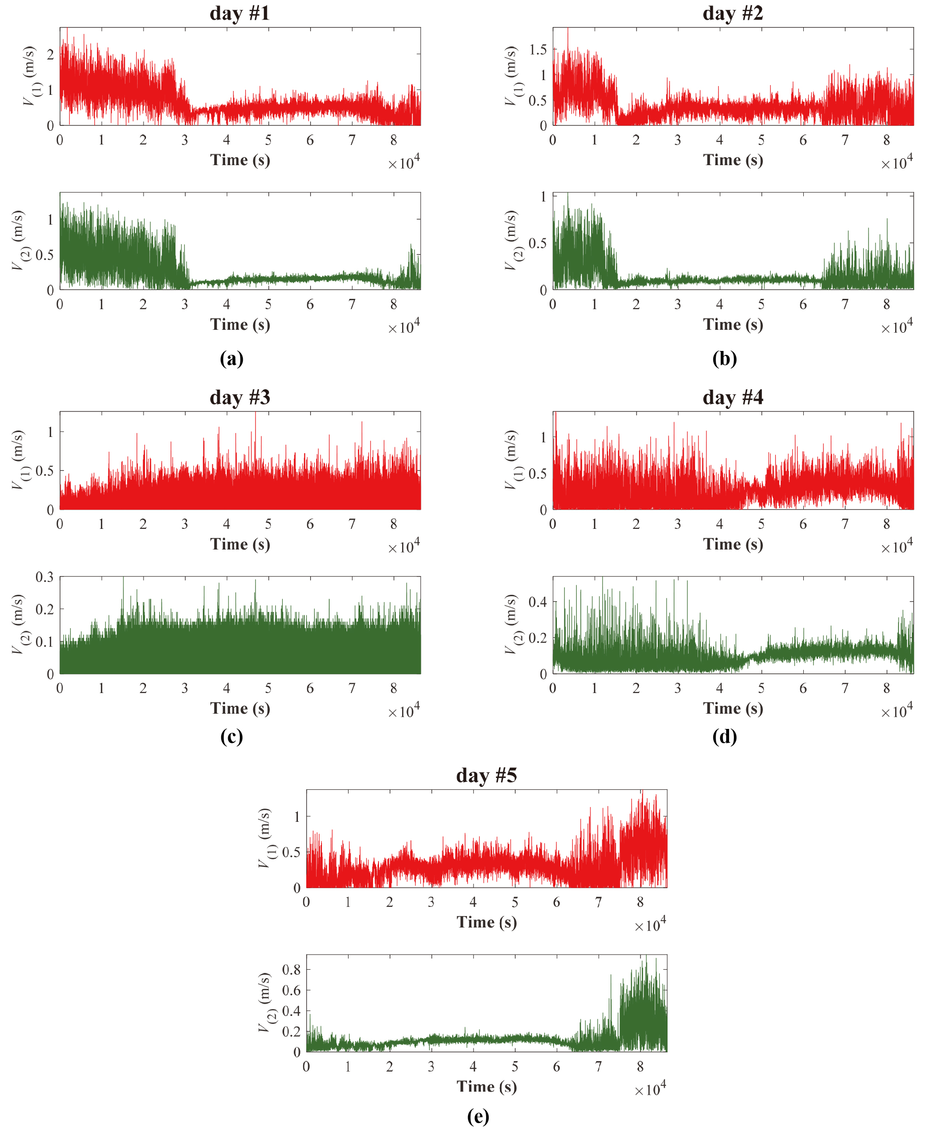
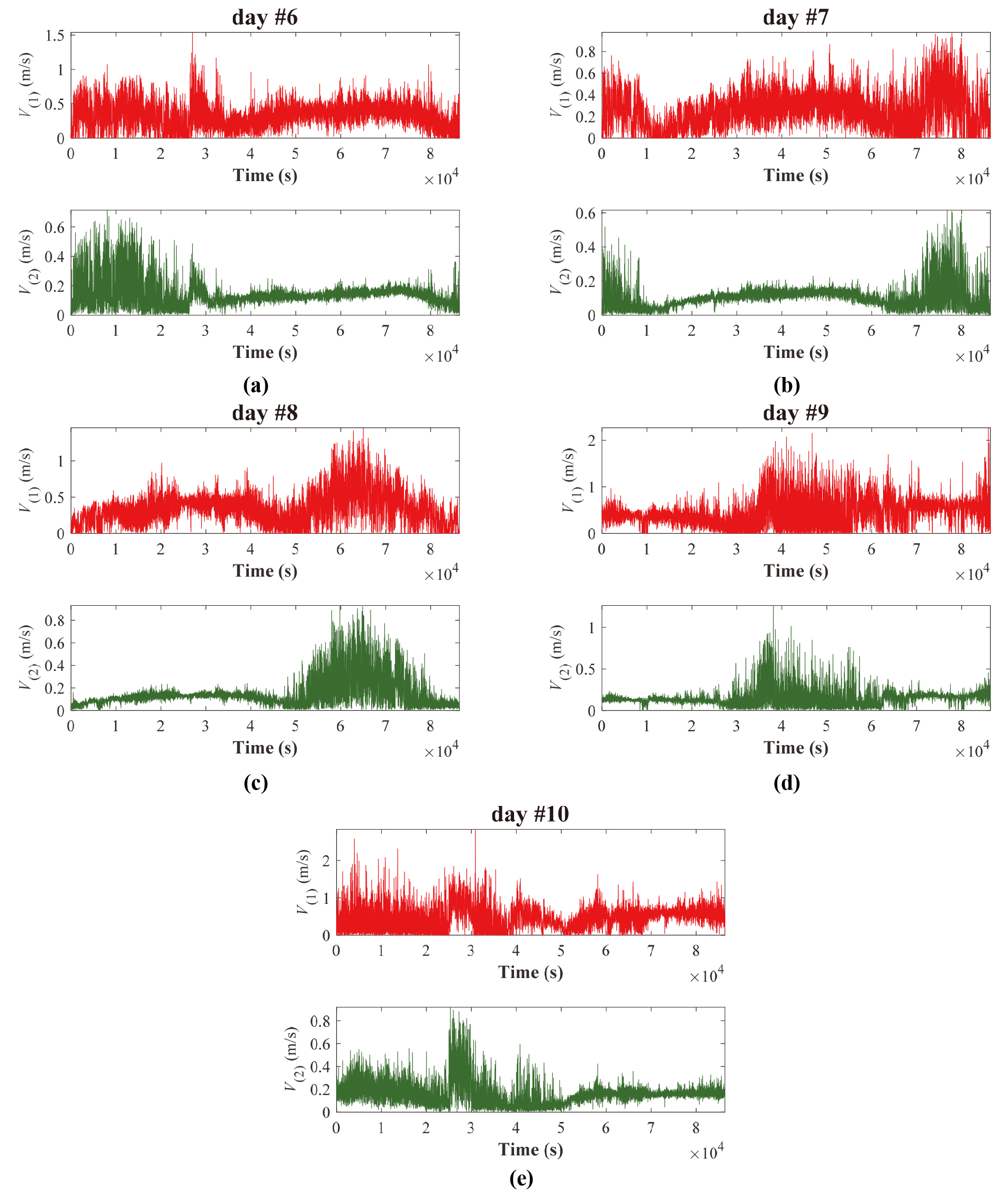
Due to some experimental difficulties, measurements were not acquired continuously. Therefore, the total measurement ensemble was divided into 10 equivalent days ( ten ensembles each consists of 86,400 numerical values). Figures 3 and 4 show the time history measurements for all ten (equivalent) days for both inlet ( $P_{1}$ ) and outlet ( $P_{2}$ ) points. In addition, surrogate time histories of measured data were developed in order to exploit a statistical approach. These time histories were relative to each second of a single synthetic equivalent-day and representative of the values obtained during the ten actual (not contiguous) days which were used as inputs at least for this first step of the study. For this purpose, 5 different approaches were explored.

Figure 3.

Days from #1 (a) to 5# (e); $V_{(1)}$ and $V_{(1)}$ velocities measurements, respectively, at the inlet point $P_{1}$ and at the outlet point $P_{2}$ .

It is easy to note the effect of atmospheric variability from Figs 3 and 4 because the velocity trends were very different day by day for both the measure points (i.e. inlet $P_{1}$ , and outlet $P_{2}$ ) as also discussed by [3]. Generally, velocities were low, ranging between 0 to 3 m/s in inlet (P1) and 0 to 2 m/s in outlet (P2). Some intervals of calm wind were observed in inlet $P_{1}$ , ranging between 1.5 $\times$ 10 ${}^{4}$ and 2 $\times$ 10 ${}^{4}$ s for day #2.

The velocity measured in $P_{1}$ was greater than that of $P_{2}$ where a great part of the measured data was smaller than 0.2 m/s. It is important to note that the lower velocity values were expected because the experimental test room had been set for passive internal ventilation. However, this occurrence did not affect the results discussed in this paper, since it focusses on the effects of the experimental data statistics on CFD model outcomes. In Section 3.2 the statistics of the series illustrated in Figs 3 and 4 are discussed.

Figure 4.

Days from #6 (a) to 10# (e): $V_{(1)}$ and $V_{(1)}$ velocities measurements respectively at the inlet point $P_{1}$ and at the outlet point $P_{2}$ .

3.2 Statistics of experimental measurements

Statistical analyses of experimental signals and numerical output time histories are discussed here so as to analyse the flow velocity variability (i.e. input and output). Working with experimental signals is a very important phase because the common purpose is to reproduce or to expand a few experimental values by using the mean value, the standard deviation or peak factors. This investigation is carried out through the signal PDF trend and consequently the Gaussianity test.

The statistics in terms of mean $V_{\mu}$ , maximum $V_{\textit{max}}$ , minimum $V_{min}$ , standard deviation $\sigma$ , skewness $\gamma_{3}$ , kurtosis $\gamma_{4}$ and peak factors (i.e. by minimum, $g_{\textit{min}}=-\frac{V_{\textit{min}}-V_{\mu}}{\sigma}$ , and by maximum, $g_{\textit{max}}=\frac{V_{\textit{max}}-V_{\mu}}{\sigma}$ ) are summarized in Table 1 for all measurement days (i.e. 10 days) and sensors ( $P_{1}$ , $P_{2}$ , $P_{3}$ ). The maxima values of peak factors $g_{\textit{max}}$ are bigger than 3.5, which is the common value given in the literature for Gaussian processes. Overall, the peak factors statistics can be surrogated by the analytical model. In the case of a Gaussian process [39], gives one of the best simulations of the experimental peak factor [40]. On the contrary, in the case of a non-Gaussian process, several analytical approaches give the experimental peak factor approximation. The analytical approach reliability depends on the specific case. For example, in the field of civil engineering, approaches given by [41, 42, 43] are successful to predict the peak factors on lateral surfaces of a high-rise building. In this research, the investigation of the Gaussianity of the measured processes was important to have a measure of the mean value significance. However, the investigation of the peak factors through the analytical model was not considered to be necessary, but this will be carefully investigated in the future.

Table 1
Statistics of velocity measurements (Ref. to Figs 3 and 4)

points	Day #	$V_{\mu}$ (m/s)	$V_{max}$ (m/s)	$V_{min}$ (m/s)	$\sigma$ (m/s)	$\gamma_{3}$	$\gamma_{4}$	$g_{\textit{max}}$	$g_{\textit{min}}$	COV
Measuring
$P_{1}$	1	0.631	2.746	0.000	0.373	0.481	3.920	5.676	1.693	0.591
	2	0.373	1.930	0.000	0.233	0.808	4.132	6.682	1.603	0.625
	3	0.130	1.270	0.000	0.175	0.716	2.629	6.516	0.743	1.346
	4	0.246	1.350	0.000	0.169	0.989	4.998	6.535	1.458	0.687
	5	0.293	1.373	0.000	0.185	0.310	4.218	5.824	1.581	0.631
	6	0.322	1.539	0.000	0.168	0.221	3.240	7.232	1.911	0.522
	7	0.252	0.977	0.000	0.159	0.307	2.922	4.563	1.582	0.631
	8	0.340	1.457	0.000	0.201	0.571	3.986	5.560	1.691	0.591
	9	0.435	2.269	0.000	0.257	0.817	5.329	7.136	1.692	0.591
	10	0.440	2.834	0.000	0.271	1.066	5.422	8.843	1.627	0.616
$P_{2}$	1	0.232	1.380	0.000	0.191	1.730	5.520	6.000	1.215	0.823
	2	0.133	1.040	0.000	0.116	2.708	11.118	7.838	1.150	1.248
	3	0.061	0.300	0.000	0.064	0.295	1.443	3.717	0.946	1.049
	4	0.096	0.539	0.000	0.048	0.993	6.892	9.260	2.006	0.499
	5	0.117	0.944	0.003	0.090	3.086	15.314	9.214	1.264	0.769
	6	0.139	0.714	0.000	0.076	1.866	9.007	7.543	1.827	0.547
	7	0.100	0.616	0.000	0.059	1.793	10.373	8.756	1.698	0.590
	8	0.143	0.931	0.000	0.113	2.139	8.378	6.956	1.263	0.790
	9	0.143	1.263	0.000	0.084	2.782	17.847	13.276	1.693	0.587
	10	0.159	0.918	0.000	0.093	1.871	10.062	8.176	1.713	0.585
$P_{3}$	1	1.679	7.033	0.000	0.890	0.301	3.750	6.013	1.886	0.530
	2	1.607	6.260	0.000	0.912	0.603	3.287	5.104	1.762	0.567
	3	0.853	5.140	0.000	1.004	0.822	2.724	4.270	0.850	1.177
	4	1.554	6.887	0.000	0.819	0.927	4.771	6.509	1.897	0.527
	5	1.308	6.742	0.000	0.853	0.843	4.052	6.374	1.534	0.652
	6	1.508	5.288	0.000	0.648	0.566	3.477	5.837	2.329	0.430
	7	1.354	4.416	0.000	0.660	0.245	3.119	4.644	2.053	0.487
	8	1.503	6.597	0.000	0.807	0.714	3.827	6.311	1.862	0.537
	9	1.634	7.905	0.000	1.011	1.127	4.785	6.203	1.617	0.619
	10	2.302	12.990	0.000	1.611	0.795	4.179	6.635	1.429	0.700

The COV index values of the measurements, which is defined as the ratio between the standard deviation of the fluctuating velocity ( $\sigma$ ) and the mean value ( $V_{\mu}$ ), was introduced. Inside the test room, the COV index related to the instrument collocated in point $P_{1}$ had values ranging from 0.522 m/s (i.e. day #6) to 1.346 m/s (i.e. day #3), whereas the measurements obtained from $P_{2}$ were ranging from 0.499 m/s (i.e. day #4) to 1.248 m/s (i.e. day #2). Outside (point $P_{3}$ ), the COV index values were between 0.430 m/s (i.e. day #6) and 1.177 m/s (i.e. day #3). The mean values ( $V_{\mu}$ ) of the time histories recorded at inlet ( $P_{1}$ ) ranged from 0.130 m/s (i.e. day #3) to 0.631 m/s (i.e. day #1). During all 10 days, the fluctuation of the mean values was significant. In fact, the standard deviation ( $\sigma$ ) of the means ( $V_{\mu}$ in Table 1) was 0.136 m/s. The maximum value of the velocity ( $V_{\textit{max}}$ ) was 2.834 m/s which was recorded during the last day of measurements. Similarly, the resulting standard deviations ( $\sigma$ ) of the ten-day series were very different from one another: from 0.159 m/s (i.e. day #7) to 0.373 m/s (i.e. day #1), confirming both day by day variability and fluctuations during the same day. Experimental values were confirmed through numerical estimations according to BS 5925:1991 [44]. Mean values between experimentally measured and numerically calculated values differed as much as 10%. Moreover, the skewness ( $\gamma_{3}$ ) and kurtosis ( $\gamma_{4}$ ) values suggested a globally non-Gaussian trend of the series. The Gaussianity of the processes was estimated through the approach given by [45] which was also adopted in [40]. According to [45], if the trend is Gaussian, the $\gamma_{3}$ and the excess kurtosis (i.e. $\gamma_{3}$ -3) should be less or equal to 0.5. Observing the data outlined in Table 1, it was noted that the measurements related to day #6 and #7 satisfied the [45] condition.

Figure 5.

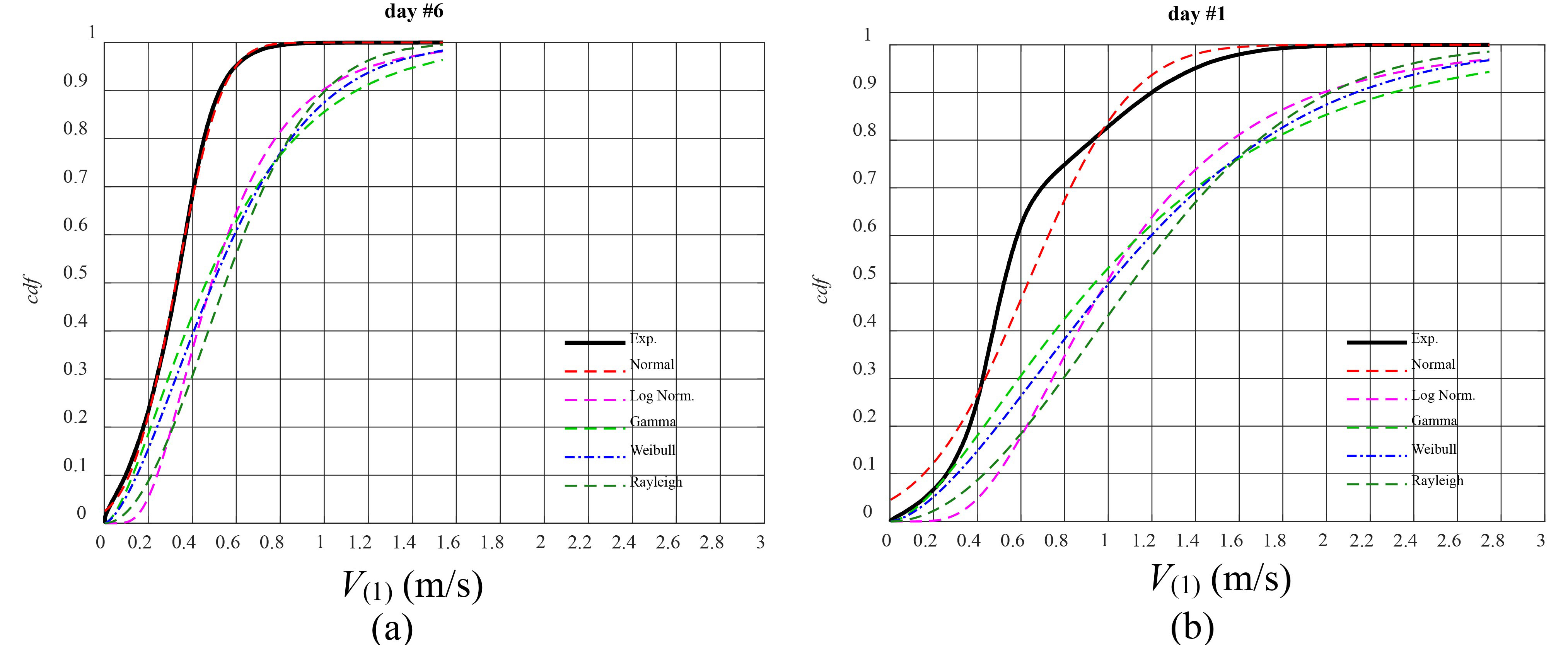
CDF of $V_{(1)}$ for day #6 (a) and day #1 (b).

This was also confirmed by the one-side Kolmogorov-Smirnov test applied on the CDF (i.e. cumulative density function) of the $V_{(1)}$ measurements. The comparison between the experimental CDF and the Normal CDF is shown in Fig. 5 for two examples, including Gaussian (i.e. day #6) process in Fig. 5a, and non-Gaussian process (i.e. day #1) in Fig. 5b. In addition, Fig. 5 shows the fitting of the empirical CDF with Weibull, Rayleigh, Gamma and Log Normal distribution.

The mean values ( $V_{\mu}$ ) of the time histories recorded in outlet ( $P_{2}$ ) ranged from 0.061 m/s (i.e. day #3) to 0.232 m/s (i.e. day #1). Similar to what was observed for $V_{(1)}$ , the fluctuation (the standard deviation) of the mean values was noteworthy, equal to 0.045 m/s, which was in any case smaller than the value obtained from $P_{1}$ measures. The maximum value of the velocity ( $V_{max}$ ) was equal to 1.380 m/s and it was recorded during the first day. Furthermore, the resulting variability of the related standard deviation was rather significant for each measurement.

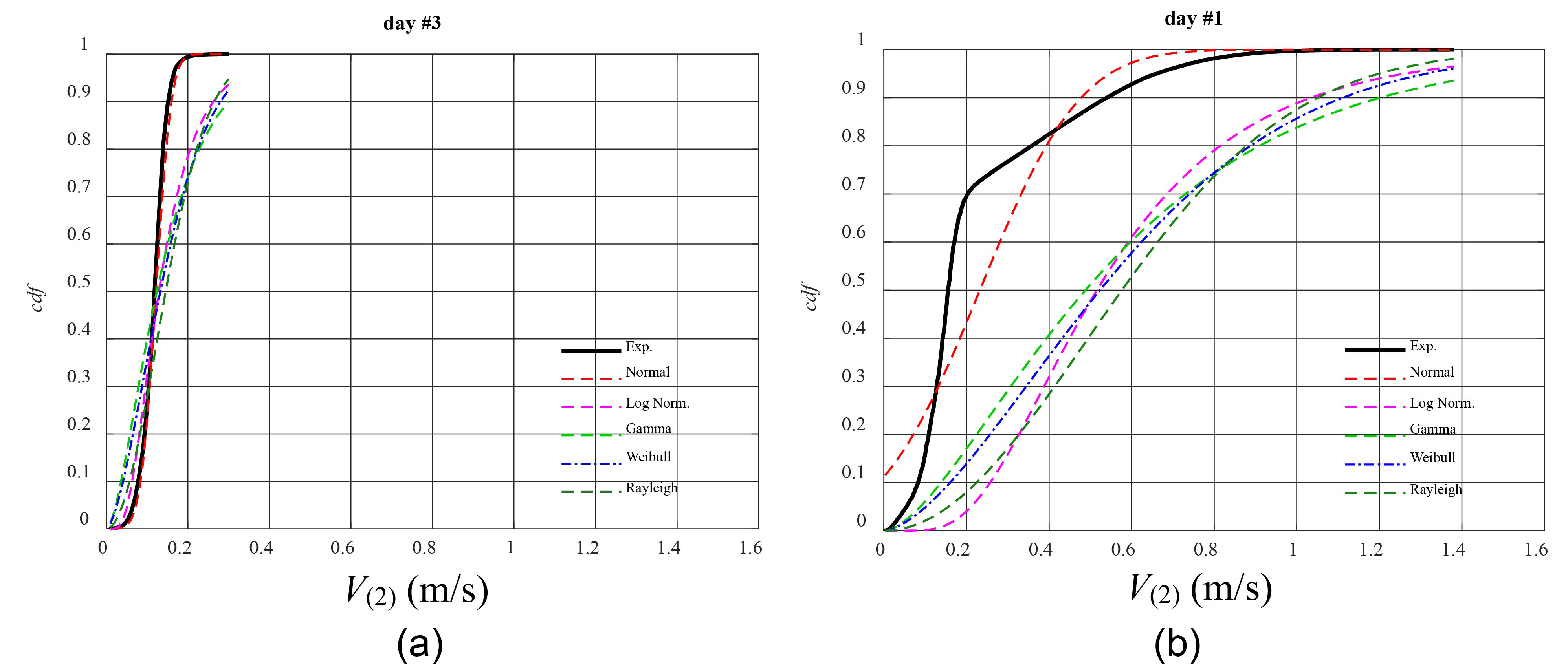
The values ranged from 0.048 m/s (i.e. day #4) to 0.191 m/s (i.e. day #1). The skewness ( $\gamma_{3}$ ) and kurtosis ( $\gamma_{4}$ ) values globally showed a non-Gaussian trend in the series. The results showed that the measurements on day #3 satisfied the [45] condition. This was also confirmed by the one-side Kolmogorov-Smirnov test applied to the cumulative density function (CDF) of the $P_{2}$ measurements.

The comparisons between the experimental CDF and the Normal CDF are shown for Gaussian (i.e. day #3) and non-Gaussian (i.e. day #1) processes in Fig. 6a and b, respectively. In particular, it is noted that the CDF illustrated in Fig. 6b and in Fig. 5b has a typical bimodal shape that is very difficult to represent by a single mode distribution.

Figure 6.

CDF of $V_{(1)}$ for day #3 (a) and day #1 (b).

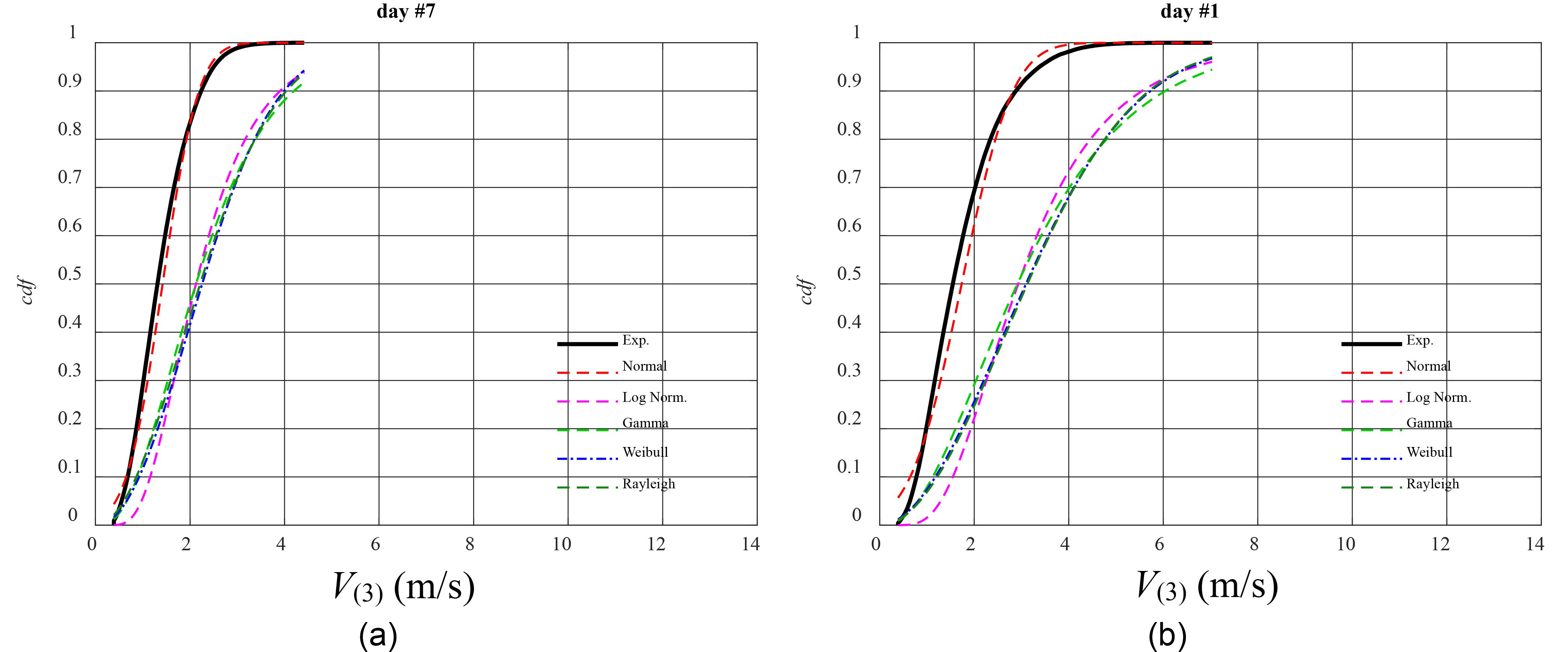
The time histories recorded by the outside sensor ( $P_{3}$ ) were characterized by a mean value ( $V_{\mu}$ ) ranging from 0.853 m/s (i.e. day #3) to 2.302 m/s (i.e. day #10). Similar to the indoor values, the fluctuation of the mean values taking place during all the analysed days was again significant and the related standard deviation was equal to 0.36 m/s. The maximum value of the velocity ( $V_{\textit{max}}$ ), which was recorded during the last day of measurements, was equal to 12.99 m/s. The standard deviation ranged from 0.648 m/s (i.e. day #6) to 1.611 m/s (i.e. day #10). The skewness ( $\gamma_{3}$ ) and kurtosis ( $\gamma_{4}$ ) values confirmed that these series were also characterized by a non-Gaussian trend except for day number 7 [45]. Figure 7a shows the empirical CDF and theoretical fittings for the time history recorded during day #7, whereas Fig. 7b shows the same for day #1. It is evident that Normal distribution gives a good fitting for empirical CDF on day #7 and it was also confirmed by the one-sided Kolmogorov-Smirnov test.

Figure 7.

CDF of $V_{(3)}$ for day #7 (a) and day #1 (b).

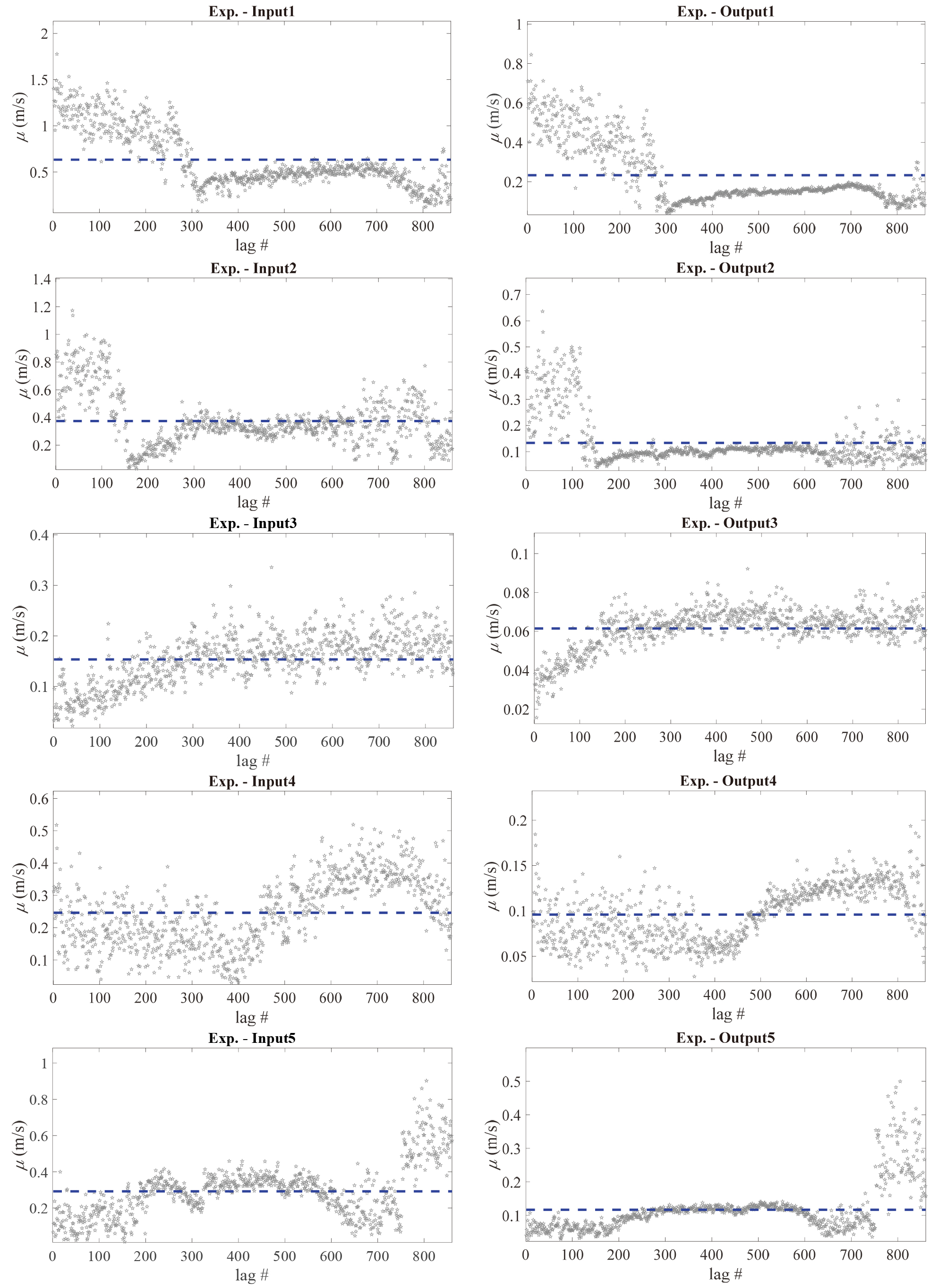
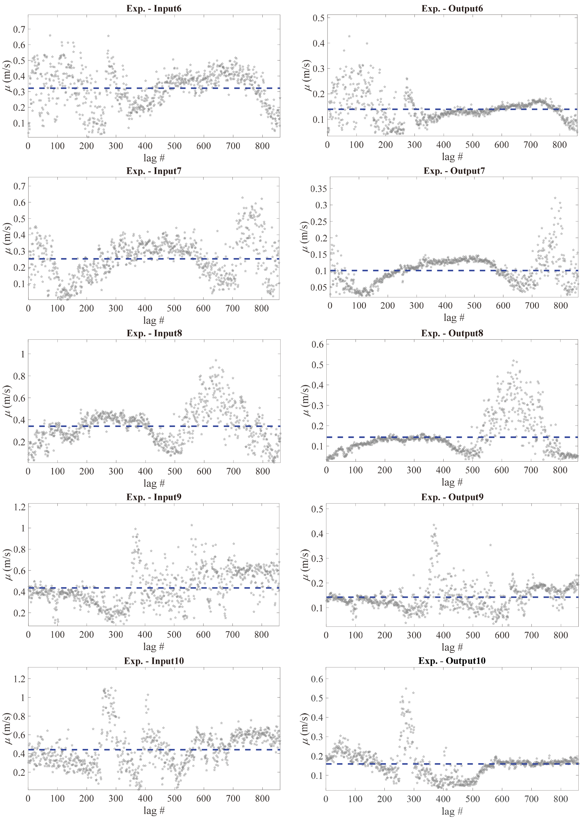
In order to have a measure of mean significance, the mean stationarity of measured signals (i.e. by sensors in $P_{1}$ , $P_{2}$ and $P_{3}$ ) was analytically estimated considering a lag equal to 100 seconds. Results show a non-stationary trend of the mean. Figures 8 and 9 show the trend for each experimental input and output measures. A similar trend is noted for variance and it can be concluded that the signals are non-stationary. This confirms that the mean signals or other statistical approximations of the full experimental database cannot surrogate the experimental measures accurately.

Figure 8.

Mean value variation for different lags for from 1 to 5 Input and Output signals measured.

Figure 9.

Mean value variation for different lags for from 6 to 10 Input and Output signals measured.

4. Fluid-dynamics simulations

In order to carry out numerical simulations of the phenomena described so far and explore how input data may affect the numerical outcomes, Unsteady Reynolds Average Navier-Stokes (URANS) simulations were carried out using the commercial CFD code ANSYS Fluent, 2013 [46] . In the following subsection, the exploited velocity inputs are discussed.

4.1 Velocity time history inputs selection

In the present research, the purpose of the experimental campaign was to acquire time histories that would be useful to calibrate a CFD numerical domain. Discussions in Section 3 have clarified that the daily measurements were statistically very different from each other. In particular, this occurrence was true for velocities measured at point $P_{1}$ , which were employed as input time histories for CFD simulations. Even if all measurements can be used as a merged input, they can be used as a representative of a few days or a month, and in any case, this requires high computational power. The purpose here is to obtain the most significant input for representative CFD analyses through statistical investigation of the measurements. The goal is to compute numerical analyses using only one input day to perform the most significant output of all measured input days. For this reason, in order to compare the numerical outcomes resulting from the CFD simulations of velocities at point $P_{2}$ with the related measured values, only one surrogate day was examined which considered to be representative of the entire experimental data set obtained at point $P_{1}$ . Accordingly, surrogate time histories of the velocity inputs (at point $P_{1}$ ), with reference to each second of the examined single “ten-day-equivalent” day, were acquired by processing the entire related experimental data from a statistical point of view. The surrogate input time histories were obtained by extracting the most important statistical information from the entire set of experimental measurements carried out at point $P_{1}$ .

Five different time history velocity inputs related to point $P_{1}$ were examined based on considerations discussed in the previous sections. The first one was the data acquired during the first measurement day (hereafter called: Input 1). For the other four input time histories, for each second of the surrogate day, different statistical combinations of the actual measurements obtained at each corresponding second of the ten days were considered. For instance, examining all the values measured on the 5400 ${}^{\rm th}$ second of each of the ten days (1:30 a.m.) can be counted as an example of this procedure. In total, 86,400 ensembles were obtained, each consisting of ten values. For each of these ensembles, four different statistical values were exploited as input data. Hence, the second time history (Input 2) was constructed by the arithmetic mean of the ten values of each ensemble, the third (Input 3) was based on the maximum value, the fourth was based on the mode (Input 4) and the fifth (Input 5) was based on Hermite polynomial chaos expansion. It is reasonable to expect that Input 3 is unrealistic because maximum values did not occur simultaneously. However, it was useful to verify the extreme values predicted by CFD simulations.

Figure 10.

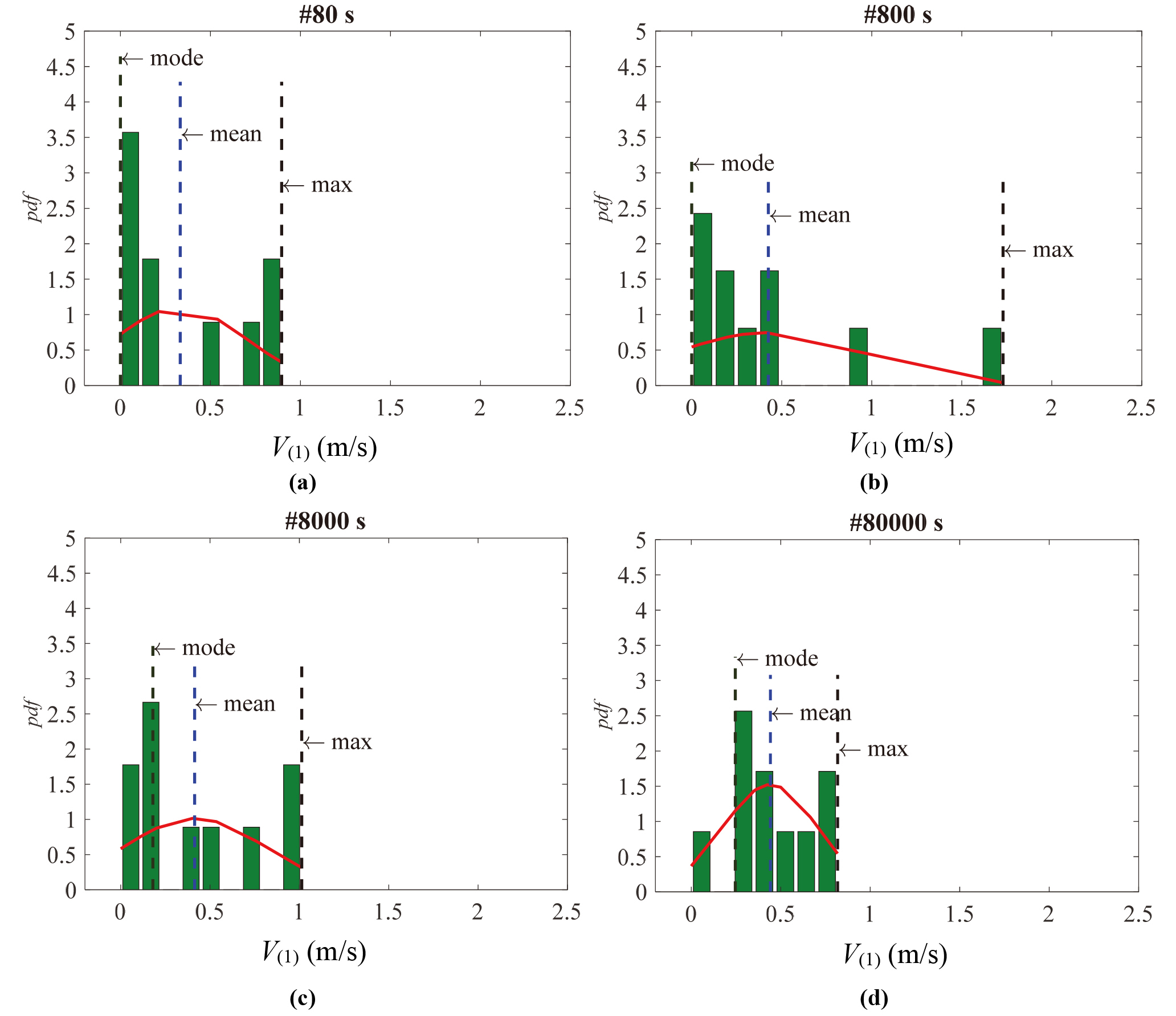
Empirical PDF of the 10 velocities measured at point $P_{1}$ on second #80 (a), #800 (b), #8000 (c) and #80,000.

Regarding Input 2, the mean values may not be considered significant for two reasons: firstly each sample corresponds for only 10 values, and secondly, since the sample may not be Gaussian, the mean would not be a good estimator. For this reason, the gaussianity of the 86,400 samples (each formed by 10 numerical values) was inspected. Figure 10 shows PDF (i.e. probability density function) related to 4 samples (each containing 10 measured values of velocities) obtained at point $P_{1}$ for randomly selected time intervals (i.e. 80, 800, 8000 and 80,000 s). The Normal distribution was overlapped in order to compare the probability distributions. From the figure, it appears clearly that the Normal distribution does not correctly represent the sample. This was confirmed by two-sided Kolmogorov-Smirnov tests on the empirical CDF. As a result, the mean was not quite representative of the sample. Similarly, both the maximum values (Input 3) and the mode values (Input 4) were not expected to be very efficient in order to acquire a satisfactory comparison between numerical results and the measured data.

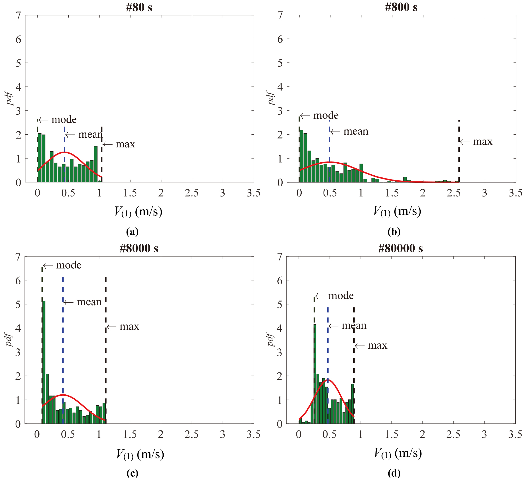
Further attempts were made for Input 5 by exploring the approach of the Polynomial Chaos Expansion (PCE) based on a spectral representation of a random variable [30]. The 10 day by day and second by second measurement samples were expanded to 365 measurement sets. Though the authors are aware that ten days are not representative of one year, this procedure was carried out to explore to what degree the results are affected by the sample size. The results are a new set of numerically generated measurements. Negative values are eliminated from the numerical data set. Figure 11 shows the PDF of the numerical data set at the same time steps illustrated in Fig. 10 (i.e. 80, 800, 8000 and 80,000 s). The Normal distribution was overlapped to the PDF, as well. The figure shows that the Normal distribution does not give a satisfactory approximation of the empirical PDF. The same trend is noted for all time steps.

Figure 11.

Empirical PDF of the 365 velocities in $P_{1}$ , numerically generated by chaos polynomial expansion, on second #80 (a), #800 (b), #8000 (c) and #80,000 (d).

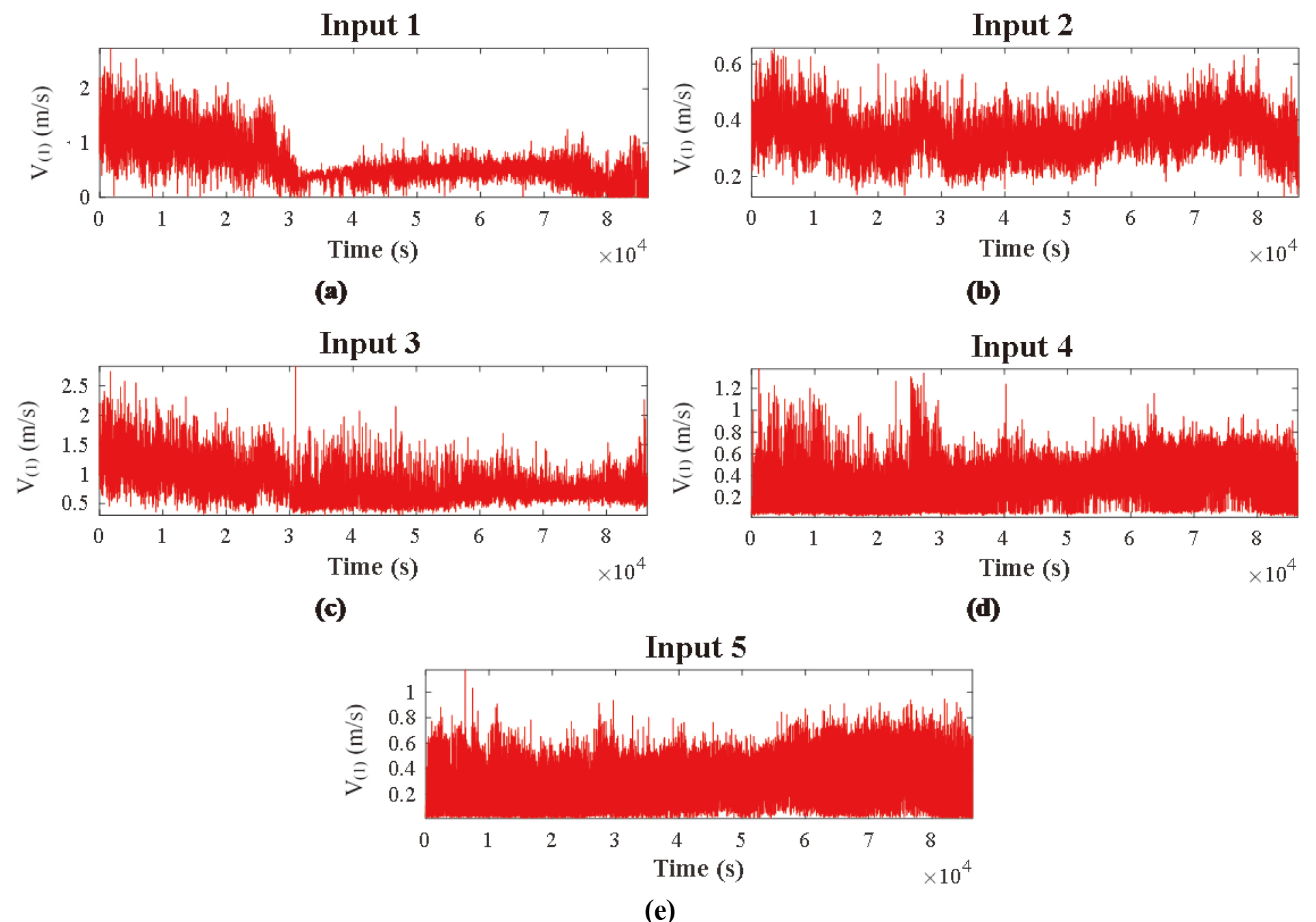
The five estimated input time histories at point $P_{1}$ used for CFD analyses are illustrated in Fig. 12 and the statistics of these time histories are summarized in Table 2. In addition, the maximum, minimum and mean values of relative error in percentage between the input time history magnitudes (i.e. mean, maximum, minimum, standard deviation, skewness, kurtosis and peak factors) and the 10-day measurements at point $P_{1}$ are listed in Table 2. The error is defined as: $\varepsilon=$ 100 $\cdot\left({V_{\textit{exp.}}-V_{\text{CFD}}}\right)/V_{\text{CFD}}$ . The mean error is estimated from the absolute values of the error. Results reported in Table 2 confirm that Input 4 and 5 give low values of mean error for all magnitudes taken into account. In particular, Input 5 (i.e. the time history given by the second after second mode of the numerically expanded sample data) gives the lowest values of mean error. In all 10-day measurements, Input 5 has mean error values (i.e. in percentage) ranging between 13.7% (i.e. peak factor) and 45.1% (i.e. skewness). These results do not guarantee that Input 5 gives an accurate CFD output at point $P_{2}$ in reference to the experimental data obtained at point $P_{2}$ . However, as will be discussed in the next sections, this is confirmed by CFD results.

Table 2

Statistics of Input time histories (Ref. to Fig. 11)

Input		$V_{\mu}$ (m/s)	$V_{\textit{max}}$ (m/s)	$\sigma$ (m/s)	$\gamma_{3}$	$\gamma_{4}$	$g_{\textit{max}}$	$g_{\textit{min}}$
		$\varepsilon$ (%)
		0.631	2.746	0.373	1.128	4.926	5.676	1.693
1	max	385.3%	181.1%	134.3%	410.4%	87.4%	24.4%	127.8%
	min	0.0%	$-$ 3.1%	$-$ 0.1%	5.8%	$-$ 9.1%	$-$ 35.8%	$-$ 11.4%
	mean	114.7%	73.4%	81.9%	132.9%	31.1%	14.8%	17.9%
2		0.348	0.656	0.068	0.239	2.898	4.549	3.266
	max	168.0%	$-$ 32.9%	$-$ 57.5%	8.2%	10.2%	$-$ 0.3%	339.6%
	min	$-$ 44.8%	$-$ 76.9%	$-$ 81.9%	$-$ 77.6%	$-$ 46.5%	$-$ 48.6%	70.9%
	mean	37.0%	58.7%	67.0%	52.3%	27.0%	27.5%	123.1%
3		0.829	2.834	0.304	1.144	4.810	6.603	1.742
	max	537.6%	190.1%	91.0%	417.6%	82.9%	44.7%	134.4%
	min	31.4%	0.0%	$-$ 18.6%	7.3%	$-$ 11.3%	$-$ 25.3%	$-$ 8.9%
	mean	182.0%	78.3%	51.9%	136.2%	29.5%	13.8%	20.7%
4		0.334	1.174	0.168	0.215	2.050	4.798	1.893
	max	156.8%	20.2%	5.3%	$-$ 2.6%	$-$ 22.0%	5.2%	154.8%
	min	$-$ 47.1%	$-$ 58.6%	$-$ 55.1%	$-$ 79.8%	$-$ 62.2%	$-$ 45.7%	$-$ 0.9%
	mean	34.9%	30.2%	19.3%	55.5%	46.9%	24.5%	29.5%
5		0.283	1.379	0.186	0.370	2.929	6.236	1.477
	max	117.8%	20.2%	5.3%	$-$ 2.5%	$-$ 25.3%	9.9%	29.8%
	min	$-$ 55.1%	$-$ 58.6%	$-$ 50.2%	$-$ 79.7%	$-$ 62.2%	$-$ 45.7%	$-$ 12.8%
	mean	32.7%	23.7%	18.1%	45.1%	26.5%	13.7%	19.1%

Figure 12.

Input 1 (a), Input 2 (b), Input 3 (c), Input 4 (d) and Input 5 (e) time history.

4.2 Implemented CFD mathematical modelling

The balance of mass, momentum and energy are the equations on which the CFD approach is built. In order to include turbulence, a very popular approach is the $k$ - $\varepsilon$ model [47, 48, 49, 50] which requests less power and time for calculation than the other approaches, such as the Large Eddy Simulation (LES) and the Direct Numerical Simulation (DNS). However, the standard $k$ - $\varepsilon$ model is actually valid only for fully turbulent flows. However, based on the main motivation and purpose of this article, this approach was selected as the first step. In the appendix, the equations and key parameters implemented in the Fluent computer code to execute the simulations discussed in this paper are briefly summarized. Essentially, the balance of mass, momentum, energy and the two turbulence equations (advection, production and dissipation of turbulent kinetic energy) were exploited. More details are reported in ANSYS Fluent, 2013 [46].

4.3 Simulations and experimental-numerical data comparison

The 3D Finite Volume Model (FVM) [52] of the room which was already implemented in the Fluent computer code was selected. The equations were integrated through a method called ‘Pressure-Based Solver’. This approach is based on an algorithm, which belongs to a general class of technique called the ‘Projection method’ [53]. The constraint of mass conservation (continuity) of the velocity field is achieved by solving a pressure (or pressure correction) equation.

The pressure equation is derived from the continuity and the momentum equations in such a way that the velocity field, which is corrected by the pressure, satisfies the continuity. The solution process involves iterations wherein the entire set of governing equations is solved repeatedly until the solution converges. The selected time step was equal to one second. In order to achieve a good balance between the computational time and result precision, preliminary simulations were repeated with different grid dimensions. Finally, the geometric domain was divided into 150,000 prismatic elements.

4.3.1 Numerical setup and main hypothesis

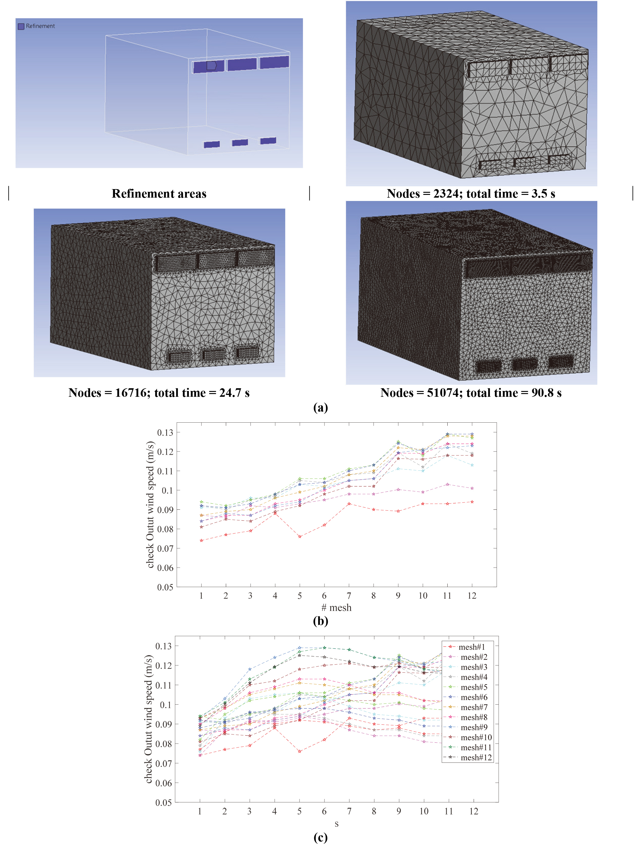
The numerical model (i.e. Fig. 13) constructed to simulate the CFD analyses in this study (i.e. Fig. 2) was a simplification of the real setup. In fact, in the numerical model (i.e. Fig. 13), the interspace (air tank and chimney, Fig. 2) through which the airflow moves into the room was neglected. Its effect was modelled through the measured inlet velocity which was applied as a time history. Thus, the airflow due to both this inlet velocity and the buoyancy forces were generated by a vertical gradient of temperature. The computational fluid domain was modelled using an inlet and an outlet velocity conditions. Figure 13 shows examples of different mesh setups and the convergence graph. As expected, the best convergence was obtained from the model with 51074 nodes mesh setup which was used for further calculations. The mesh size ranges from 9.6 $\times$ 10 ${}^{-4}$ to 9.6 $\times$ 10 ${}^{-2}$ m.

The room was modelled as a prismatic volume. As illustrated in Fig. 2, for the full-scale setup, the test room at full-scale consists of three walls made of plasterboard, a floor and a roof ceiling made of brick elements, and an aluminum and glass window. Polystyrene panels were applied on the outside surface of the glass window to simulate the soil effect. In the numerical model scale (Fig. 12), all surfaces were simulated taking into account the heat exchange between inside the test room and outside.

The three walls and the floor surfaces were modelled with a constant temperature value of 23 ${}^{\circ}$ C which was obtained from site measurements. The wall density, specific heat and thermal conductivity coefficients were assumed to be equal to 1100 kg/m ${}^{3}$ , 840 J/kgK and 0.36 W/mK, respectively. The floor was modelled as an equivalent surface with a density equals to 1600 kg/m ${}^{3}$ , the specific heat coefficient of 1000 J/kgK and the thermal conductivity coefficient of 0.80 W/mK. The glass window and the polystyrene layers were modelled as an equivalent layer with a density value equals to 35 kg/m ${}^{3}$ , the specific heat coefficient equals to 1700 J/kgK and the thermal conductivity coefficient equals to 0.034 W/mK.

The initial condition used for the first time step of the unsteady analysis was computed through the measurements and the values in literature. The density was assumed to be equal to 1186 kg/m ${}^{3}$ . The specific heat coefficient and the thermal conductivity coefficient were taken as 1007 J/kgK and 0.026 W/mK, respectively. 1.51 $\cdot$ 10 ${}^{-5}$ Pa $\cdot$ s of viscosity and 50% of relative humidity values were adopted. This condition varied step by step as a function of the temperature gradient.

The room temperature distribution varied step by step as a function of the inlet velocity, outside temperature and the heat exchange with all surfaces. These effects provided a vertical temperature gradient and buoyancy forces, consequently. All these conditions were confirmed through measurements and the numerical domain was calibrated based on the test room conditions. During the measurements were taken, the temperature outside the room was lower than that of inside all the time. Even though this condition was expected for nighttime only, it was also observed during the daytime thanks to a polystyrene layer. Based on these measurements, the inlet temperature was assumed to be equal to 20 ${}^{\circ}$ C. It is reasonable to expect that this condition will change from month to month and these assumptions can be considered invalid for a different period of the year. However, it is worth noting that the goal of this paper was to give a statistical approach to compute CFD simulations of ventilation through measurements.

Figure 13.

CFD model grid: different modelling (a), graph of convergence for different modelling setup (b) and Outlet velocity trends at different seconds of calculation for each mesh setup.

5. Analyses results

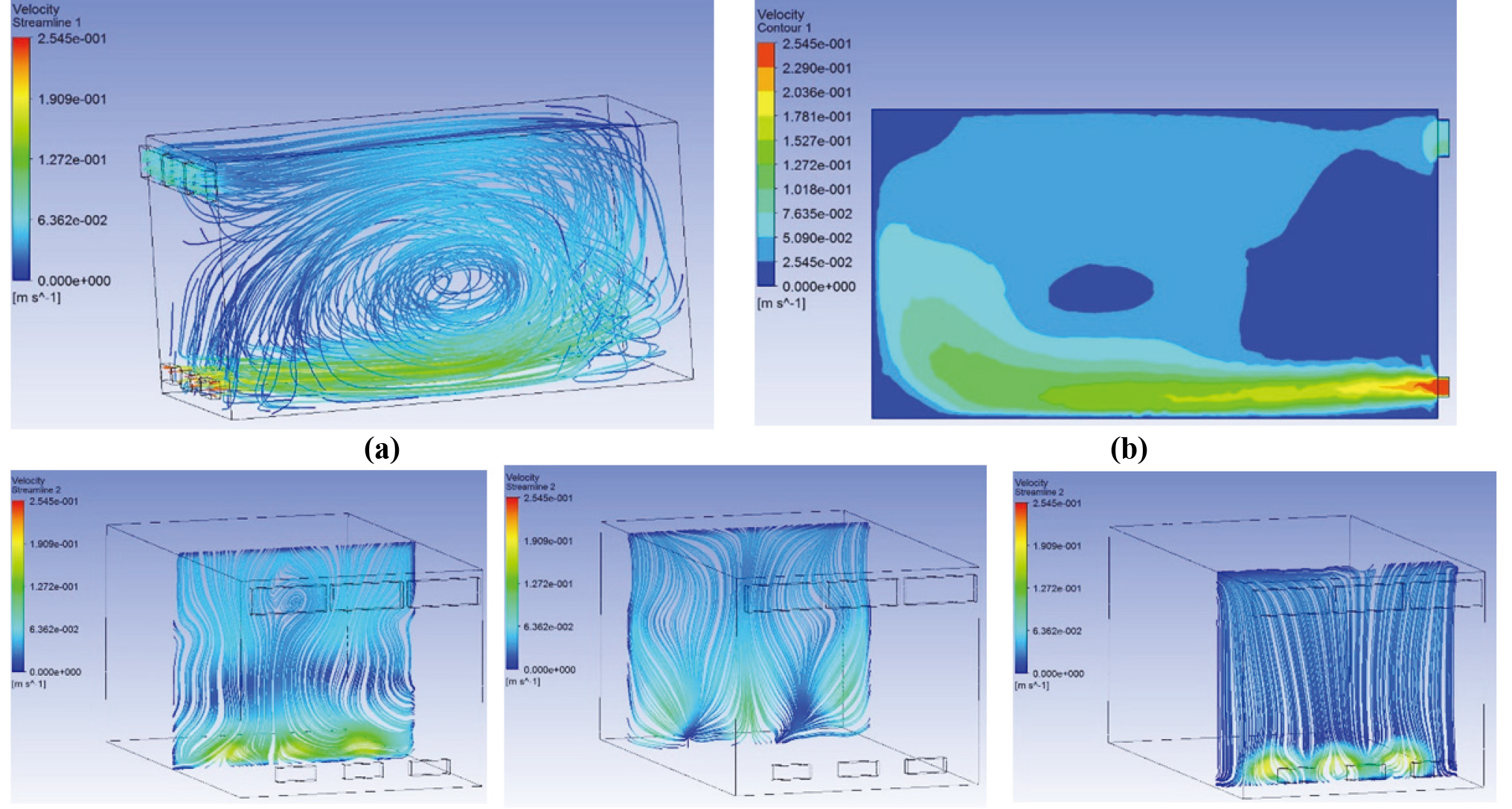
The initial attempt involved exploring Input 1 and selecting day #1. Consequently, the velocity data measured at point $P_{2}$ (Fig. 3) were compared with the corresponding velocity outcomes of the numerical simulation at the same $P_{2}$ point for day #1. The RMSE (root mean square error) was used to measure the correspondence between numerical and experimental data. The total inlet temperature and pressure, as well as the static outlet pressure were imposed at the domain boundaries based on the mean value of the measurements. Figure 13 shows the model grid used for CFD calculations. Figure 14 shows some significant results of the CFD simulations. In particular, the vector velocity 3D trends and the velocity streamlines for different room cross-sections are shown in Fig. 14a and b, respectively.

Table 3
Correlation coefficients ( $C$ ) between $V_{(1)}$ (Input) and $V_{(1)}$ (Output) time histories

Experimental	$C$	Cfd simulation	$C$
Day #		Input/output
1	0.91	1	0.28
2	0.78	2	0.01
3	0.90	3	0.31
4	0.67	4	0.36
5	0.78	5	0.60
6	0.69	7	0.69
8	0.79
9	0.66
10	0.60
max	0.91
min	0.60
mean	0.75

Figure 14.

CFD velocity contours plot: 3D (a) and 2D cross-section plot, different cross sections velocity streamlines at 1m, 2.5 m and 4 m distant from the air Inlet area.

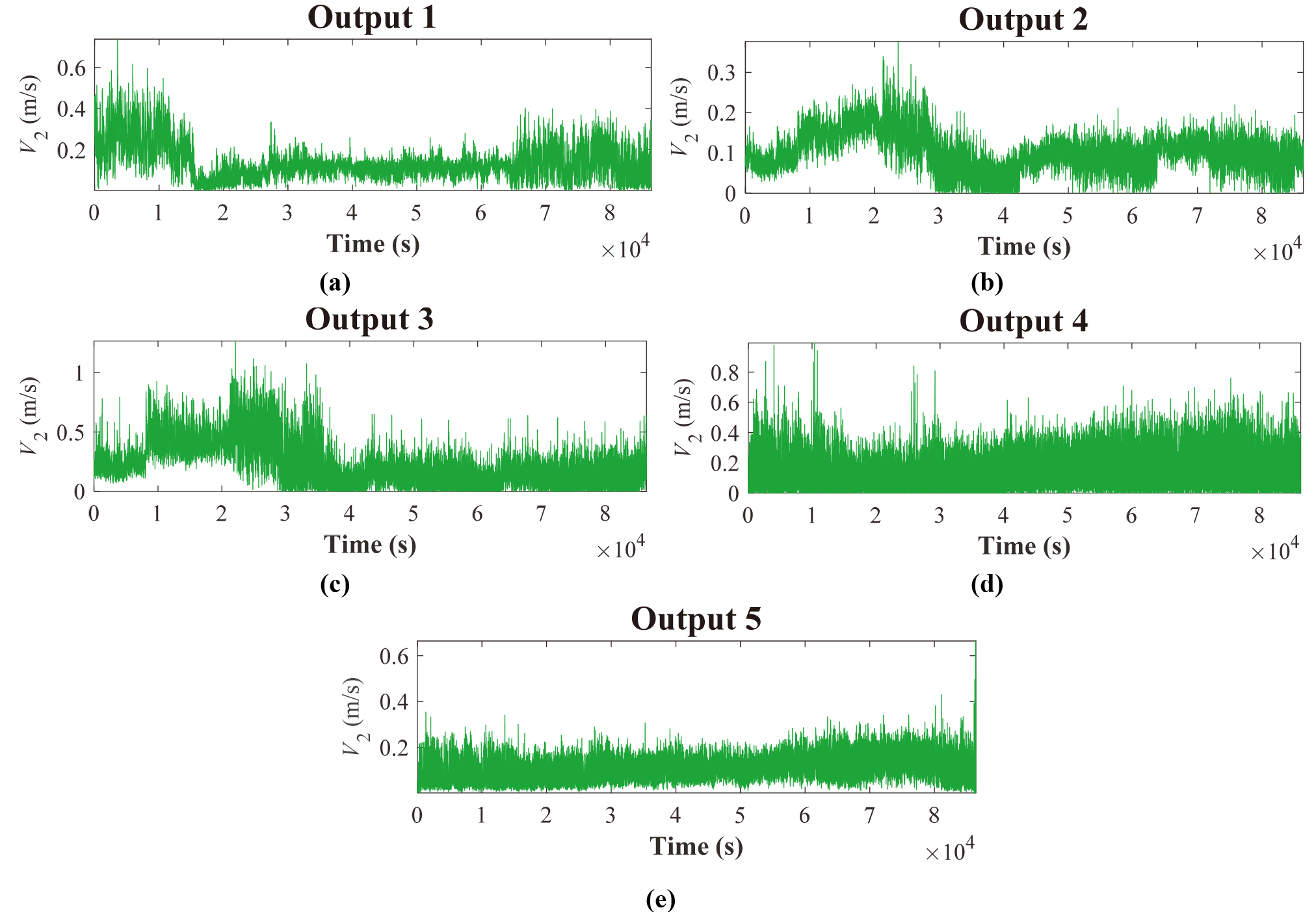
Following an optimal configuration of the CFD model grid obtained after grid independence was reached, analyses were repeated using all the selected input data (i.e. input from 1 to 5). In the following, Output 1 to 5 represent the $V_{(1)}$ time history calculated by CFD analyses using input 1 to 5. Figure 15 shows the output time histories numerically generated by CFD simulations. In the same way, as was done for input time histories, CFD output time histories were compared with measurements at point $P_{2}$ for all days (Figs 3 and 4).

Table 4

Statistics of the CFD results

Output		$V_{\mu}$ (m/s)	$V_{\textit{max}}$ (m/s)	$\sigma$ (m/s)	$\gamma_{3}$	$\gamma_{4}$	$g_{\textit{max}}$	$g_{\textit{min}}$
		$\varepsilon$ (%)
		0.136	0.738	0.099	1.260	8.649	10.903	1.615
1	max	122.1%	146.1%	107.3%	327.2%	499.4%	193.3%	70.7%
	min	$-$ 41.6%	$-$ 46.5%	$-$ 47.9%	$-$ 59.2%	$-$ 51.5%	$-$ 17.9%	$-$ 19.5%
	mean	28.6%	38.5%	37.2%	68.4%	73.7%	52.7%	24.6%
		0.103	0.377	0.046	0.486	3.402	5.957	2.237
2	max	68.5%	25.6%	$-$ 4.2%	64.7%	135.8%	60.3%	136.4%
	min	$-$ 55.7%	$-$ 72.7%	$-$ 75.9%	$-$ 84.3%	$-$ 80.9%	$-$ 55.1%	11.5%
	mean	28.7%	52.7%	43.4%	73.5%	70.8%	30.6%	59.7%
		0.238	1.265	0.167	1.238	3.952	6.157	1.428
3	max	290.5%	321.6%	247.5%	319.5%	173.9%	65.6%	51.0%
	min	2.7%	$-$ 8.3%	$-$ 12.7%	$-$ 59.9%	$-$ 77.9%	$-$ 53.6%	$-$ 28.8%
	mean	101.7%	77.6%	107.8%	68.3%	69.3%	29.4%	21.8%
		0.139	0.992	0.103	1.252	4.462	8.394	1.347
4	max	127.6%	230.6%	114.8%	324.5%	209.2%	125.8%	42.4%
	min	$-$ 40.2%	$-$ 28.1%	$-$ 46.0%	$-$ 59.4%	$-$ 75.0%	$-$ 36.8%	$-$ 32.9%
	mean	29.3%	48.8%	40.0%	68.4%	67.9%	26.7%	20.5%
		0.112	0.664	0.056	0.927	5.088	7.969	1.306
5	max	83.5%	84.0%	114.8%	26.1%	$-$ 7.8%	32.8%	13.5%
	min	$-$ 51.7%	$-$ 51.9%	$-$ 70.8%	$-$ 65.8%	$-$ 75.0%	$-$ 36.8%	$-$ 32.9%
	mean	27.6%	38.1%	34.6%	67.5%	66.2%	24.8%	19.9%

Figure 15.

CFD Output 1 (a), Output 2 (b), Output 3 (c), Output 4 (d) and Output 5 (e) time history.

Figure 16.

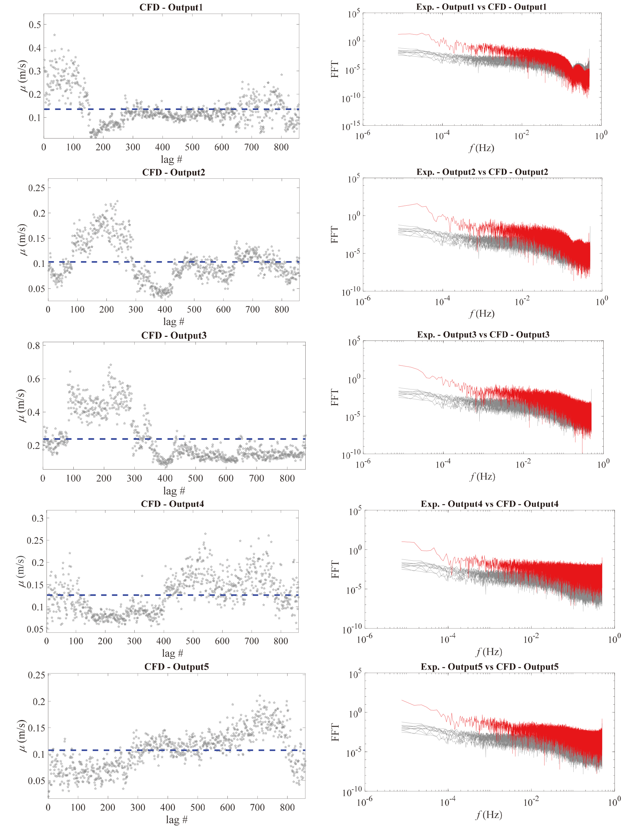
Mean value variation for different lags for from CFD Output signals and comparison between FTT of experimental (i.e. gray curves) and numerical Output signals (i.e. red curves).

In order to define a measure of agreement between input and output time histories, the correlation coefficients ( $C$ ) between the time histories at $P_{1}$ and $P_{2}$ for both numerical and experimental data sets are reported in Table 3. $C$ is calculated through Eq. (2), where $A$ and $B$ are two generic time depending processes.

$\displaystyle C\left({A,B}\right)=\frac{1}{N-1}\sum_{i=1}^{N}\left({\frac{% \overline{A_{i}-\mu_{A}}}{\sigma_{A}}}\right)\left({\frac{\overline{B_{i}-\mu_% {B}}}{\sigma_{B}}}\right)$ (2)

The correlation coefficients between the experimental measurements and the numerical results were compared for both data series acquired at inlet (P1) and outlet (P2). It was found that the experimental values measured for 10 days give a correlation coefficient ranging from 0.91 to 0.60 with a mean value of 0.75. These values are significantly large suggesting that the flow field from inlet to outlet is not disturbed. On the contrary, the correlation coefficients estimated between inlet and outlet series in numerical analyses are particularly small. The biggest value is given between Input 5 (i.e. generated through PCE) and Output 5 and it is equal to 0.6. This result confirms the eligibility of Input 5 values generated by chaos polynomials. Finally, statistics regarding CFD output time histories were compared with the experimental data statistics at point $P_{2}$ . Table 4, similarly to Table 2, presents the statistics of the CFD output time histories together with the min, max and mean errors in percentage between the numerical and experimental outputs.

Output 5 (i.e. CFD Output 5 resulting from Input 5 which was numerically generated by chaos polynomials) gives the best result in terms of mean error of the statistics. The mean error ( $\varepsilon$ %) of the mean value ( $V_{\mu}$ ) is similar for all outputs except for Output 3 (i.e. coming from Input 3, based on maximum values of each second) and it ranges from 27.6% (i.e. Output 5) to 29.3% (i.e. Output 4). The value obtained from Output 3 is equal to 101% which is much greater than the others.

The mean error ( $\varepsilon$ %) of the maximum value ( $V_{\textit{max}}$ ) varies from 38.1% (i.e. Output 5) and 77.6% (i.e. Output 3). Values for Output 1, 2, 4 and 5 are similar to each other. The mean error ( $\varepsilon$ %) of the standard deviation ( $\sigma$ ) ranges from 34.6% (i.e. Output 5) to 107.8% (i.e. Output 3). In addition, the mean values assumed by the $\sigma$ variance, related to Output 1, 2, 4 and 5 ranges from 34.6% (i.e. Output 5) to 43.4% (i.e. Output 2). The mean error ( $\varepsilon$ %) of the skewness and kurtosis is globally greater than others and all outputs give similar values. The Mean error ( $\varepsilon$ %) of the skewness varies from 67.5% (i.e. Output 5) to 73.5% (i.e. Output 2), whereas the mean error ( $\varepsilon$ %) of the kurtosis ranges from 66.2% (i.e. Output 5) to 73.7% (i.e. Output 1). Table 4 shows that the skewness and kurtosis of experimental data are not satisfactorily reproduced by all CFD numerical values. Finally, the mean error ( $\varepsilon$ %) for peak factors (i.e. $g_{\textit{min}}$ and $g_{\textit{max}}$ ) is found to be acceptable because it ranges between 24.8% (i.e. Output 5) and 52.3% (i.e. Output 1) for $g_{\textit{max}}$ ; and between 19.9% (i.e. Output 5) and 59.7% (i.e. Output 2), respectively for $g_{\textit{min}}$ . Figure 15 shows that the numerical output signals preserve a non-stationary trend. In addition, the comparison between the FFT of experimental output measurements (i.e. gray curves) and the numerical output signals (i.e. red curves) shows a satisfactory agreement for Output 4 and 5.

6. Conclusions

In this paper, the effect of an experimental statistics data set on the numerical outcomes of a selected CFD simulation was investigated. An ensemble of air velocity values, which were measured for each second over ten days at both inlet and outlet locations in a 5.2 $\times$ 3.4 $\times$ 2.7 m room, were exploited as test cases. CFD analyses were executed with different time histories of inlet velocities, in order to compare numerical and experimental outlet time histories. Respectively, the selected inputs were: a single day of measurement (i.e. Input 1), a mean value time history (i.e. Input 2), a maximum value time history (i.e. Input 3), a mode value time history (i.e. Input 4) and a mode time history of a numerically expanded (by chaos polynomials) data set (i.e. Input 5). Overall results show that the experimental signals are not stationary and that mean, maximum and minimum of the measured signals are not significantly affected by the measurement processes.

A preliminary comparison between the statistics (i.e. mean, maximum, minimum, standard deviation, skewness, kurtosis and peak factors) of measurements and input time histories were given in terms of the mean error in percentage. Results show that the Input 5 statistics were closer to the experimental data set statistics than others. Similarly, the CFD output (i.e. in outlet) time history statistics were compared with the corresponding measurements in the outlet. The results confirm that Input 5 gives the best approximation of the experimental data statistics. The reason is that the expansion by chaos polynomials gives a greater data set based on experimental data set seed and this increases the possibility to determine the statistics of the ten experimental data sets. However, the analyses also showed that using different inputs resulted in significant variability between the obtained results. Accordingly, the study highlights the importance of selecting the input for CFD analysis, which applies to the calibration process even more. The main conclusion, from the aforementioned arguments is that one should investigate different cases separately in order to determine the most significant input for each specific case to perform numerical analyses. However, it is worth mentioning that the results presented in this paper are obtained from a specific case study. Further research and analyses are required to generalize findings.

Footnotes

Appendix

References

Minson

A.J.

, Use of laser doppler anemometer measurements near model buildings to determine wind loading on building attachments, D. Phil Thesis, University of Oxford, 1993.

Minson

A.J.

Wood

C.J.

and Belcher

R.E.

, Experimental velocity measurements for CFD validation, Journal of Wind Engineering and Industrial Aerodynamics 58 (1995), 205–215.

Schatzmann

and Leitl

, Issues with validation of urban flow and dispersion CFD models, Journal of Wind Engineering and Industrial Aerodynamics 99 (2011), 169–186.

Lee

I.B.

Okushima

Ikeguchi

Sase

and Short

T.H.

, Prediction of natural ventilation of multispan greenhouses using CFD techniques and its verification with wind tunnel test, In: the 2000 ASAE 93r⁢d Annual International Meeting, Milwaukee, USA, July 9–12, 2000.

Mamou

Tahia

Benmeddour

Cooper

K.R.

Abdallah

Khalid

and Fitzsimmons

, Computational fluid dynamics simulations and wind tunnel measurements of unsteady wind loads on a scaled model of a very large optical telescope: A comparative study, Journal of Wind Engineering and Industrial Aerodynamics 96 (2008), 257–288.

Abdelrazaq

Kijewski-Correa

Song

Y.H.

Isyumov

and Kareem

, Design and full-scale monitoring of the tallest building in Korea: Tower Palace II. In: The Sixth Asian-Pacific Conference on Wind Engineering, 2004.

van Hooff

and Blocken

, Full-scale measurements of indoor environmental conditions and natural ventilation in a large semi-enclosed stadium: Possibilities and limitations for CFD validation, Journal of Wind Engineering and Industrial Aerodynamics 104–106 (2012), 330–341.

Gan

and Riffat

S.B.

, CFD modelling of air flow and thermal performance of an atrium integrated with photovoltaics, Building and Environment 39 (2004), 735–748.

Hertwig

, Dispersion in an urban environment with a focus on puff releases, Study Project, University of Hamburg, Meteorological Institute, 2008.

10.

Cook

M.J.

and Hanby

, CFD modelling of natural displacement ventilation in an enclosure connected to an atrium, Building and Environment 42 (2007), 1158–1172.

11.

Cook

and Hunt

, CFD modelling of buoyancy-driven natural ventilation opposed by wind, Ninth International IBPSA Conference, Montréal, Canada, August 15–18, 2005.

12.

Leitl

and Schatzmann

, Validation data for urban flow and dispersion models – are wind tunnel data qualified? In: Proceedings of the Fifth International Symposium on Computational Wind Engineering (CWE2010), Chapel Hill, North Carolina, USA, May 23–27, 2010.

13.

Repschies

Leitl

and Schatzmann

, Validation of urban dispersion models: how representative are locally measured wind velocities? In: Proceedings of the 10th Annual George Mason University Conference on Atmospheric Transport and Dispersion Modeling. Fairfax VA, USA, August 1–3, 2006.

14.

Allwine

K.J.

Leach

M.J.

Stockham

L.W.

Shinn

J.S.

Hosker

R.P.

Bowers

J.F.

and Pace

J.C.

, Overview of JOINT URBAN2003 an atmospheric dispersion study in Oklahoma City, In: Proceedings of the AMS Symposium on Planning, Nowcasting, and Forecasting in the UrbanZone, January 11–15, 2004, Seattle, Washington, USA.

15.

Fry

, Experimental data and design, and the role of statistics, Surgery 27(9) (2009), 375–380.

16.

Jordan

M.A.

Powell

and Phillips

C.V.

, Experimental data analysis: a guide to the selection of sample statistical tests, Minerals Engineering 10(3) (1997), 275–286.

17.

Calista

Pasculli

and Sciarra

, Reconstruction of the geotechnical model considering random parameters distributions, Engineering Geology for Society and Territory, 353(1) (2015), 1347–1351.

18.

Hanna

S.R.

Brown

M.J.

Camelli

F.E.

Chan

S.T.

Coirier

W.J.

Kim

Hansen

O.R.

Huber

A.H.

and Reynolds

R.M.

, Detailed simulations of atmospheric flow and dispersion in downtown Manhattan: an application of five computational fluid dynamics models, Bulletin of the American Meteorological Society 87(12) (2006), 1713–1726.

19.

Sepe

Rizzo

Ricciardelli

and Avossa

A.M.

, Characterization of mean wind profiles and surface roughness assessment from wind LIDAR measurements, In: Proceedings of the Italian Association for Wind Engineering conference (IN-VENTO XV), September 9

{}^{\rm th}

–12

{}^{\rm th}

2018, Naples (Italy), 2018.

20.

Vu-Bac

Lahmer

Zhuang

Nguyen-Thoi

and Rabczuk

, A software framework for probabilistic sensitivity analysis for computationally expensive models, Advances in Engineering Software 100 (2016), 19–31.

21.

Hamdia

K.M.

Silani

Zhuang

and Rabczuk

, Stochastic analysis of the fracture toughness of polymeric nanonparticle composites using polynomial chaos expansions, International Journal of Fracture 206 (2017), 215–227.

22.

Pasculli

, Viscosity variability impact on 2D laminar and turbulent Poiseuille velocity profiles; Characteristic-Based Split (CBS) stabilization, In: the 5th Int. Conf. On Mathematics and Computers in Sciences and Industry MCSI2018, August 25–27, Corfù, Greece, 2018.

23.

Hall

R.C.

, WS Atkins Consultants Ltd, Woodcote Grove, Ashley Road, Epsom, Surrey KT18 5BW, UK1997.

24.

Ketzel

Berkowicz

Muller

W.J.

and Lohmeyer

, Dependence of street canyon concentrations on above roof wind speed – implications for numerical modelling, International Journal of Environment and Pollution 17 (2002), 356–366.

25.

Di Crescenzo

, Meccanismi di scambio termico tra aria e terreno e ventilazione naturale in edifici interrati, Studio numerico e sperimentale di un prototipo in scala reale (in Italian). Graduate thesis, G. D’Annunzio University, Chieti-Pescara, 2018.

26.

Rizzo

Caracoglia

and Montelpare

, Predicting the flutter speed of a pedestrian suspension bridge through examination of laboratory experimental errors, Engineering Structures 172 (2018), 589–613.

27.

Rizzo

and Caracoglia

, Examining wind tunnel errors in Scanlan derivatives and flutter speed of a closed-box, Journal of Wind and Structures 26(4) (2018), 231–251.

28.

Rizzo

and Caracoglia

, Artificial Neural Network model to predict the flutter velocity of suspension bridges, Computers and Structures 233 (2020), 106236.

29.

Rizzo

Ricciardelli

Maddaloni

Bonati

and Occhiuzzi

, Experimental error analysis of dynamic properties for a reduced-scale high-rise building model and implications on full-scale behaviour, Journal of Building Engineering 28 (2019), 101067.

30.

Ghanem

and Spanos

P.D.

, Stochastic Finite Elements: A Spectral Approach, Springer-Verlag, New York, New York, USA, 1991.

31.

Grigoriu

, Stochastic calculus, Applications in science and engineering, Birkhäuser, Boston, MA, USA, 2002.

32.

Xiu

and Karniadakis

G.E.

, The Wiener-Askey polynomial chaos for stochastic differential equations, SIAM Journal on Scientific Computing 24(1) (2002), 619–644.

33.

Schoefs

Yáñez-Godoy

and Lanata

, Polynomial chaos representation for identification of mechanical characteristics of instrumented structures, Computer-Aided Civil and Infrastructure Engineering 26(3) (2011), 173–189.

34.

Desceliers

Soize

and Ghanem

, Identification of chaos representations of elastic properties of random media using experimental vibration tests, Computational Mechanics 39(6) (2007), 831–838.

35.

Gurley

and Kareem

, Analysis, interpretation, modeling and simulation of unsteady wind and pressure data, Journal of Wind Engineering and Industrial Aerodynamics 69-71 (1997), 657–669.

36.

Ding

and Chen

, Assessment of methods for extreme value analysis of non-Gaussian wind effects with short-term time history samples, Engineering Structures 80 (2014), 75–88.

37.

Canor

Caracoglia

and Denoël

, Application of random eigenvalue analysis to assess bridge flutter probability, Journal of Wind Engineering and Industrial Aerodynamics 140 (2015), 79–86.

38.

Caracoglia

, An Euler-Monte Carlo algorithm assessing Moment Lyapunov Exponents for stochastic bridge flutter predictions, Computers & Structures 122 (2013), 65–77.

39.

Davenport

A.G.

, Note on the distribution of the largest value of a random function with application to gust loading, Proceedings of the Institution of Civil Engineering 28(1) (1964), 187–196.

40.

Rizzo

Barbato

and Sepe

, Peak factor statistics of wind effects for hyperbolic paraboloid roofs, Engineering Structures 173 (2018), 313–330.

41.

Kwon

and Kareem

, Peak Factors for Non-Gaussian Load Effects Revisited, Journal of Structural Engineering 137(12) (2011), 1611–1619.

42.

Walpole

Myers

and Ye

, Probability and Statistics for Engineers and Scientists, 9

{}^{\rm th}

edition, Upper Saddle River, NJ, USA: Pearson - Prentice Hall, 2002.

43.

Huang

M.F.

Lou

Chan

C.M.

Lin

and Pan

, Peak distributions and peak factors of wind-induced pressure processes on tall buildings, Journal of Engineering Mechanics 139(12) (2013), 1744–1756.

44.

BS 5925:1991, Code of practice for Ventilation principles and designing for natural ventilation.

45.

Suresh Kumar

and Stathopoulos

, Wind loads on low building roofs: a stochastic perspective, Journal of Structural Engineering 126(8) (2000), 944–956.

46.

ANSYS Fluent. Release 15.0. Theory Guide. November, Ansys Inc., 2013.

47.

Launder

B.E.

and Spalding

D.B.

, Lectures in Mathematical Models of Turbulence, Academic Press, London, England, 1972.

48.

Chung

T.J.

, Computational Fluid Dynamics, Cambridge University Press, 2006.

49.

Pasculli

, CFD-FEM 2D Modelling of a local water flow. Some numerical results, Alpine and Mediterranean Quaternary 21(B), (1), (2008), 215–228.

50.

Richards

P.J.

and Hoxey

R.P.

, Appropriate boundary conditions for computational wind engineering models using the k–e turbulence model, Journal of Wind Engineering and Industrial Aerodynamics 46-47 (1993), 145–153.

51.

Pasculli

Calista

and Sciarra

, Variability of local stress states resulting from the application of Monte Carlo and finite difference methods to the stability study of a selected slope, Engineering Geology 245 (2018), 370–389.

52.

Versteeg

H.K.

and Malalasekra

, An Introduction to Computational FluidDynamics, The Finite Volume Method, Longman Scientific & Technical, Harlow, England, 1995.

53.

Chorin

A.J.

, Numerical solution of Navier-Stokes equations, Mathematics of Computation, 22 (1968), 745–762.

Statistical approach to compute a surrogate input for building physics CFD simulations through experimental measurements

Abstract

Keywords

1. Introduction

2. Methodology

3.1 Experimental setup

Table 1 Statistics of velocity measurements (Ref. to Figs 3 and 4)

4.1 Velocity time history inputs selection

4.3 Simulations and experimental-numerical data comparison

4.3.1 Numerical setup and main hypothesis

Table 3 Correlation coefficients ( C ) between V ( 1 ) (Input) and V ( 1 ) (Output) time histories

Footnotes

Appendix

References

Table 1
Statistics of velocity measurements (Ref. to Figs 3 and 4)

Table 3
Correlation coefficients ( $C$ ) between $V_{(1)}$ (Input) and $V_{(1)}$ (Output) time histories