Development of look-ahead NURBS interpolation based on the exponential function

Abstract

Aiming at the problem of large number of points and complex calculation of NURBS pre-interpolation, this paper puts forward a look-ahead interpolation with offline feedrate optimization. The NURBS interpolator is divided into two stages: pre-interpolation and real-time interpolation. The pre-interpolation preprocesses the curve segment by segment according to the curvature characteristics, at the same time the exponential function method is adopted during the pre-interpolation in the look-ahead module. This method makes the step increment of interpolation parameters change exponentially in the area with gentle curvature, and greatly reduces the number of pre-interpolation points, which reduces the amount of calculation and improves the real-time performance. The real-time interpolation stage adopts the bidirectional adaptive acceleration and deceleration control method to realize speed smoothing without needing to calculate the deceleration point. The simulation results show that the real-time performance of the algorithm is greatly improved.

Keywords

NURBS interpolation look-ahead interpolation exponential function

1. Introduction

A nonuniform rational B-spline (NURBS) curve unifies analytic graphics and free shape with a general mathematical expression and is determined as the only expression form of free parts and products by the ISO. In fact, it has become the standard of industrial CAD geometric modeling. NURBS curve interpolation technology has many obvious advantages, such as small data storage, complete information, and smooth speed. High-speed and high-precision machining is easily realized [1, 2] and has been widely used to describe and machine complex parts in modern CNC systems [3, 4].

NURBS interpolation is a research hotspot of CNC in recent years. Shpitalni et al. [5] used the Taylor series expansion algorithm for parametric curve interpolator with a constant feedrate. However, this method has large contour error at sharp corners and is not practical. Yeh and Hsu [6] developed an adaptive feedrate interpolation which adjusted the feedrate based on curvatures and confined chord errors. Tikhon et al. [7] considered the constant material removal rate to improve machining accuracy and proposed an improved adaptive interpolation method, the performance of adaptive interpolation method is further improved. Park et al. [8] developed a real-time NURBS interpolation based on the two-stage method which can make good use of the geometric characteristics of NURBS. Tsai et al. [9] presented an acceleration/deceleration method before interpolation, thus the interpolation accuracy is improved. In order to improve the interpolation performance, some interpolation algorithms combined with the dynamic characteristics of machine tools are proposed. Yong and Narayanaswami [10] developed an interpolation by detecting sharp corners based on chord error information in offline. Sencer et al. [11] proposed an optimization method of feed speed considering axis constraints. However, frequent acceleration and deceleration changes may cause jerk out of tolerance. Nam and Annoni [12, 13] considered the influence of Jerk and proposed the Jerk-limited feedrate planning. Beudaert et al. [14] Considered the 5-axis NURBS jerk constraints and proposed 5-axis feedrate NURBS interpolation. Nam and Yang [15] developed a generalized parametric interpolator with real-time jerk-limited acceleration. Jahanpour and Alizadeh [16] proposed a novel acc-jerk-limited NURBS interpolation enhanced with an optimized S-shaped quintic feedrate scheduling scheme. Wei et al. [17] developed a NURBS interpolator which maintains constant speed at federate sensitive regions considering drive and contour-error constraints. Liu et al. [18] presented an adaptive feedrate planning with geometric and kinematic constraints, effectively improved the accuracy of interpolation.

In addition, due to the continuous influence of NURBS curve curvature, feedrate planning has always been the key problem of NURBS interpolation. Erkorkmaz et al. [19] proposed a federate optimization based on linear programming and windowing. Wang et al. [20] developed an adaptive smooth feedrate scheduling to solve the problem of feedrate fluctuation. Chen and Sun [21] presented a contour error-bounded parametric interpolator for five-axis CNC machine tools with minimum feedrate fluctuation. Zhong et al. [22] proposed a new real-time interpolator, which adjusted the look-ahead length dynamically to minimize the calculation load and kept the feed rate as high as possible with minimum fluctuation. Zhang et al. [23] developed adaptive feedrate planning with an iterative method that considered the error and higher-order kinematic constraints, but the real time could not be guaranteed. Ni et al [24] proposed a jerk-continuous NURBS interpolation using the polynomial and trigonometric functions to construct the jerk-continuous ACC/DEC profile, improved the flexibility of feedrate control.

The above NURBS interpolation methods are usually based on a single processor. The shorter the interpolation time of NURBS curve, the smaller the interpolation point distance and the higher the machining accuracy. A high-speed and high-precision interpolation cycle generally must be controlled at the millisecond level, which imposes higher requirements for the real-time performance of the interpolator. Considering the mechanical, electrical and system performance factors in the actual processing process, the feed speed cannot always be kept constant, so flexible acceleration and deceleration control is needed. However, because the NURBS curve is constructed by the B-spline basis function, no exact mathematical relationship holds between arc length and parameters in the interpolation process of the NURBS curve, so accurate control of the acceleration and deceleration is difficult. Therefore, more functional modules must be added to realize smooth interpolation, which makes the system load grow exponentially.

In order to improve the real-time performance of pre-interpolation and the interpolation accuracy, this paper proposes a real-time NURBS interpolation method based on a two-level interpolation mechanism. The NURBS interpolator is divided into two stages: pre-interpolation and real-time interpolation. The first stage of pre-interpolation preprocesses the curve segment by segment according to the curvature characteristics and obtains the initial and final parameter vector, feed speed, and length of the curve segment. The second stage of real-time interpolation adopts a two-way speed planning method, which improves the performance of the acceleration and deceleration modules and improves the accuracy of deceleration point positioning as much as possible. According to the de Boor recursive algorithm, the interpolation points are generated in real time. In the pre-interpolation stage, the exponential function is used to control the increment of step size, which greatly reduces the number of interpolation points, thus effectively reducing the computational complexity of preprocessing. At the same time, the speed planning method can well control the speed fluctuation of interpolation, effectively improve the accuracy of interpolation and realize the purpose of high-speed and high-precision machining.

2. The concept of interpolation of the NURBS curve

A $p$ -degree NURBS curve is defined as:

$\displaystyle C(u)=\frac{\sum\limits_{i=0}^{n}{N_{i,p}(u)w_{i}P_{i}}}{\sum% \limits_{i=0}^{n}{N_{i,p}(u)w_{i}}}$ (1)

where the index $i=$ 0, 1, $\ldots$ , $n$ ; {Pi} is the set of control points; { $\omega_{i}$ } is the set of weights; {Ni, $p(u)$ } is the set of $p$ -order $B$ -spline basic functions defined on the nonuniform knot vector $U$ . The first and last weight factors satisfy the condition of $w_{0}>0$ and $w_{n}>0$ , respectively, and the remaining factors meet the conditions $w_{i}\geqslant 0$ , where $u$ is the independent variable of the NURBS curve.

NURBS curve interpolation indicates that in each interpolation cycle, the spatial position points that should be reached in the next cycle are calculated. Therefore, the key requirement is the corresponding parameter $u$ . In general, the Taylor series expansion method is used to expand parameter $u$ with respect to time $t$ .

$\displaystyle u_{i+1}=u_{i}+\left.{\frac{du}{dt}}\right|_{t=t_{i}}T+\left.{% \frac{1}{2}\frac{d^{2}u}{dt^{2}}}\right|_{t=t_{i}}T^{2}+\textit{H.O.T}$ (2)

$T$ represents the interpolation period, and H.O.T represents the higher-order term of the Taylor expansion.

$v(u_{i})$ is the feedrate corresponding to point $C(u_{i})$ , which can be obtained by the displacement increment and time increment as follows:

$\displaystyle v(u_{i})=\left\|{\frac{dC(u)}{dt}}\right\|_{u=u_{i}}=\left\|{% \frac{dC(u)}{du}}\right\|_{u=u_{i}}\left.{\frac{du}{dt}}\right|_{t=t_{i}}$ (3)

The first-order approximate expression of parameter u as a function of t can be obtained by transforming Eq. (3):

$\displaystyle\left.{\frac{du}{dt}}\right|_{t=t_{i}}=\frac{v(u_{i})}{\left\|{% \frac{dC(u)}{du}}\right\|_{u=u_{i}}}$ (4)

Then, the second-order approximate expression of parameter $u$ as a function of time $t$ is obtained as:

$\displaystyle\left.{\frac{d^{2}u}{dt^{2}}}\right|_{t=t_{i}}=-\frac{v^{2}(u_{i}% )T^{2}\left.{\left({\frac{dC(u)}{du}\cdot\frac{dC^{2}(u)}{du^{2}}}\right)}% \right|_{u=u_{i}}}{\left\|{\frac{dC(u)}{du}}\right\|_{u=u_{i}}^{4}}$ (5)

The parameters of the next interpolation point can be calculated using the parameters and feedrate of the current interpolation point according to Eqs (2), (4) and (5). Then, the interpolation point coordinates can be calculated using the de Boor fast algorithm.

The increment of the parameter step can be obtained by the difference between parameters of adjacent interpolation points as follows:

$\displaystyle\Delta u=u_{i+1}-u_{i}$ (6)

$\Delta u$ is the increment of the parameter step, $u_{i}$ is the parameter of current point, $u_{i+1}$ is the parameter of the next point. The main purpose of pre-interpolation is to calculate the parameters of each pre-interpolation point through Taylor series expansion. In the pre-interpolation process, the interpolation parameter increment is a very critical parameter. The pre-interpolation process is essentially a discrete process for the normalized parameter vector 0 $\sim$ 1. The fewer processing points are required, the less geometric information of the curve can be obtained. A reasonable choice of step increment can not only reduce the number of processing points, improve the processing speed, but also obtain enough geometric information of the curve. If the increment of the parameter step can be controlled, the calculation cost of pre-interpolation can be well controlled.

3. Structure of the NURBS interpolation

Figure 1.

Structure of the NURBS curve interpolator.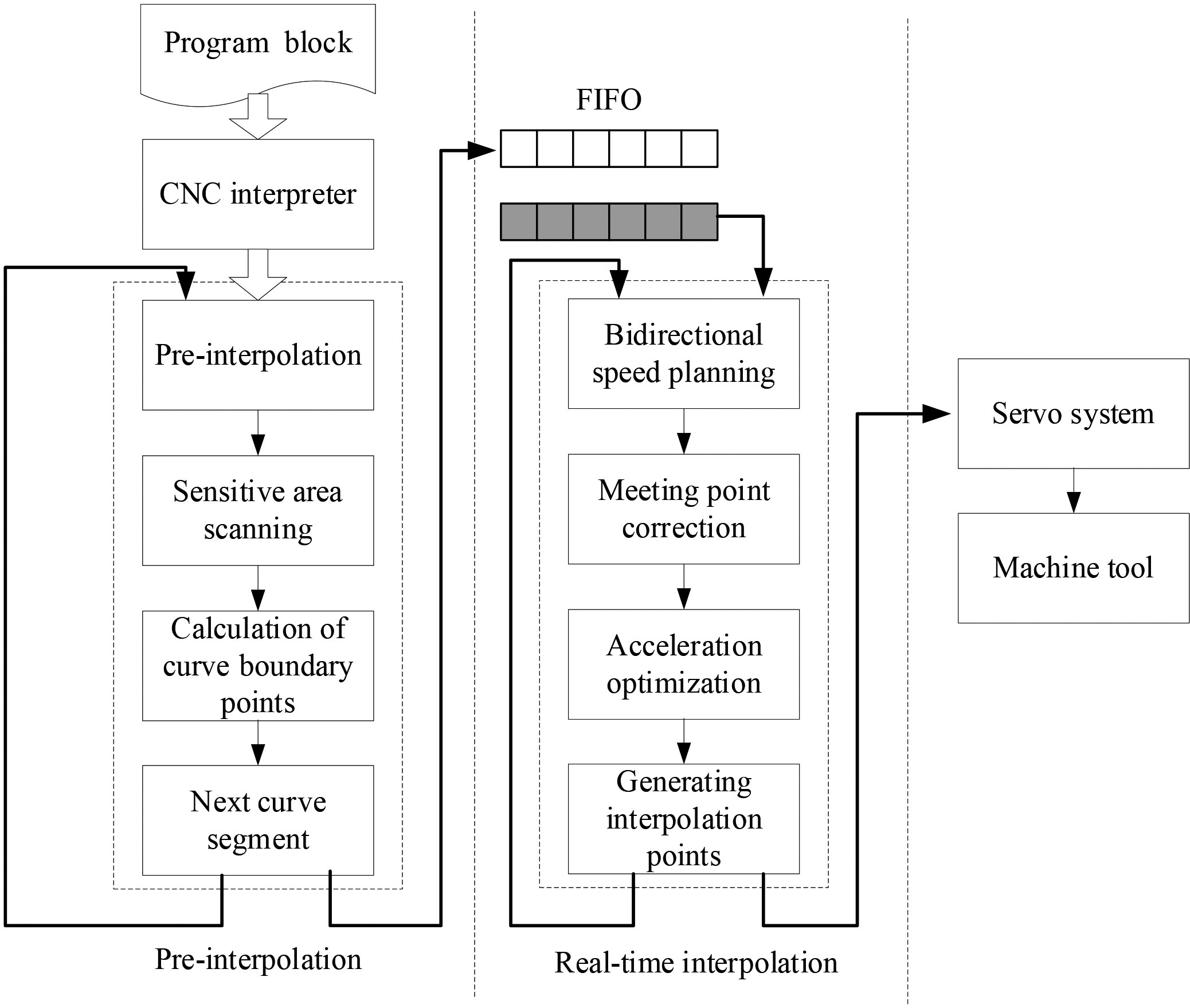

The NURBS interpolator proposed in this paper is shown in Fig. 1. The interpolation is divided into two stages: pre-interpolation and real-time interpolation. The pre-interpolation mainly performs the preprocessing of interpolation, while the real-time interpolation completes the real-time interpolation. The first-level pre-interpolation transfers data to the second-level real-time interpolation through first in first out (FIFO) queue. Preprocessing and real-time interpolation are independent, and the two stages can run on the hardware platform with a master-slave structure, such as PC-FPGA and ARM-FPGA. Pre-interpolation is performed on the master CPU, and real-time interpolation is performed on the slave motion control chip to achieve load balancing.

In the first stage of pre-interpolation, the CNC interpreter reads in the program block, analyzes the NC code file and extracts the workpiece information described by the NURBS curve; the fast pre-interpolation module makes the parameter increment increase rapidly according to the binary index in the flat curvature section, to realize the fast pre-interpolation of the NURBS curve; in the curvature mutation area, the Taylor expansion method is used to calculate the parameters and pre-interpolate at the normal speed; the speed is sensitive The sensing area scanning module judges the starting point and end point of the speed-sensitive point according to the basic information of the fast pre-interpolation point, to form the sensitive area information; the curve segment boundary point calculation module obtains the segmented boundary point approximately according to the reference interval of the speed-extreme point and the curvature extreme point of the feedrate sensitive area; finally, the segmented curve information is saved, including the boundary point parameter vector, feed speed, curve segment length, etc. It is put into the FIFO queue for the second level real-time interpolation.

In the second stage of real-time interpolation, the information of the curve segment to be processed is read from FIFO queue to obtain the starting point parameters, feedrate, and length of the curve segment; the speed planning module interpolates the curve segment from the positive and reverse directions to constrain the feed speed at the same time, the forward interpolation is output to the servo system in real time, and the reverse interpolation buffers the interpolation data points to the FIFO queue; and the forward and reverse interpolation is implemented. After arriving at the convergence area, calculate the transition point and adjust its feed speed to make the acceleration of positive and negative interpolation at the transition point zero; when the positive interpolation reaches the transition point, output the interpolation point from the LIFO queue to the servo system to drive the machine tool to feed.

4. Pre-interpolation

Because of the limitations of machine tool mechanical characteristics, processing requirements, electrical response frequency and other factors, the feedrate cannot always remain constant. Without losing generality, it is assumed that the processing speed curve is continuous, and the speed change is from low to high and then to low. Before moving to the minimum speed, we must slow down; before moving to the maximum speed, to improve the processing efficiency, we should accelerate as much as possible. To reduce the velocity fluctuation, each curve segment consists of only one acceleration phase and one deceleration phase (the middle segment may contain a constant speed phase).

Based on the above analysis, the NURBS curve can be segmented according to the corresponding relationship between velocity and curvature, which is the main task of first-level pre-interpolation. The first-level pre-interpolation and the second-level real-time interpolation should transmit data through FIFO queue. The former interpolation must ensure that FIFO queue has data to avoid starvation.

4.1 Fast pre-interpolation

The basic idea of fast pre-interpolation is that the parameter step increment adapts to the changes in the geometric characteristics of the curve. In the flat curvature, because it can meet various constraints, the parameter vector can be quickly discretized with a larger step increment. Here we choose the exponential function (binary) is used to make the parameter step increment rapidly increase, and at the sudden change of curvature to meet the constraints such as contour error in real time, the geometric information of the curve is obtained with a small step increment.

The curve of NURBS can be roughly divided into a large curvature region and a small curvature region. The influence of curvature on chord error is as follows:

$\displaystyle\textit{ER}_{i}=\rho_{i}-\sqrt{(\rho_{i})^{2}-\left(\frac{v(u_{i}% )\cdot\mbox{T}}{2}\right)^{2}}$ (7)

where $\rho_{i}$ is the radius of curvature, $T$ is the interpolation cycle, and $v(u_{i})$ is the feedrate of $C(u_{i})$ .

$\displaystyle\rho_{i}=1/k_{i}$ (8)

where $k_{i}$ is the curvature.

Equations (7) and (8) show that the chord error is smaller in the large curvature area and larger in the small curvature area of the NURBS curve. The idea of fast pre-interpolation is that different calculation methods are used for interpolation point parameter vectors according to different curvature regions of the NURBS curve. In the large curvature region, because the chord error can meet the limitation of the maximum chord error, the adjacent interpolation points can be far away; that is, the parameter increment can be larger, so the parameter vector of the interpolation points can be calculated by increasing the parameter increment in a binary exponential way. In the small curvature region, because the chord error may exceed the limit of the maximum chord error, the distance between adjacent points should be small; that is, the parameter increment can be small. The first-order Taylor expansion approximation method is used to directly calculate the parameters of the vector. The specific flow of the algorithm is shown in Fig. 2.

Figure 2.

Flow chart of fast pre-interpolation.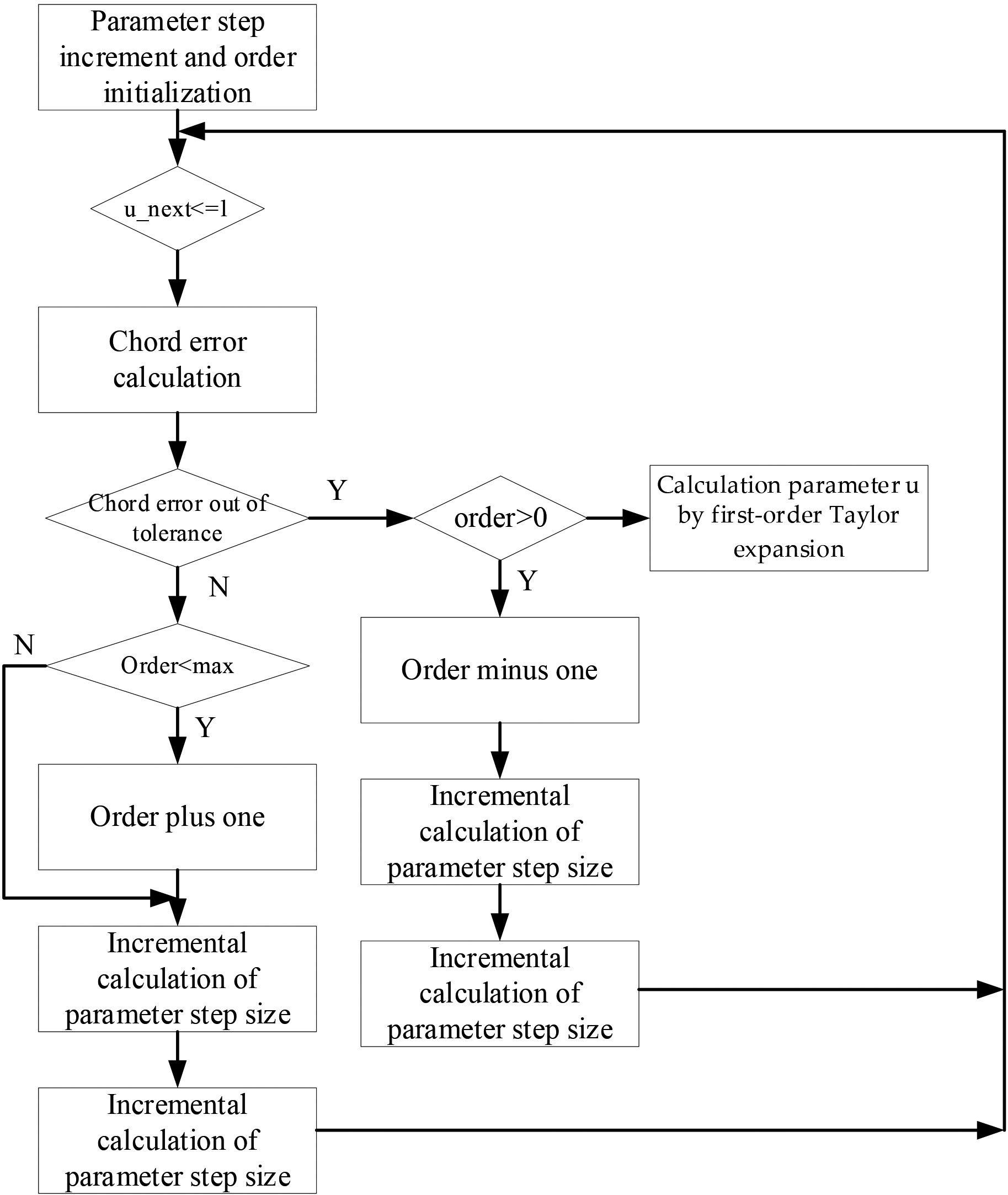

When the increment of the parameter step is a binary exponential increment, its growth rate is very fast. If it is not controlled, the distance between adjacent pre-interpolation points will be too long, and some feedrate sensitive areas of the curve may be skipped. Therefore, the maximum order of the binary exponent must be limited.

In addition, when the new interpolation point is calculated according to the parameter vector and parameter step increment of the current pre-interpolation point, its chord error is out of tolerance. At this time, it is not clear that the interpolation has entered the abrupt curvature region from the large curvature region. Perhaps the parameter step increment is larger, and the subsequent part of the large curvature region is skipped, so the parameter step increment must be readjusted. The adjustment rule is as follows: from this point forward, the increment of each calculated parameter step should be reduced to half of the original value until the parameter step increment is reduced to the initial setting value. If the chord error of the new interpolation point calculated by the increment of the initial parameter step remains out of the limit, then the point is the starting point of the curvature mutation region, and then the parameter vector is calculated using the first-order Taylor expansion method

4.2 Calculation of segment boundary points

The chord error is determined by the curvature radius and feed speed. When the radius of curvature is large, the chord error may exceed the limit. To meet the requirement of chord error, the feed speed should be adjusted.

$\displaystyle v(u_{i})=\frac{2}{T}\sqrt{\delta_{\max}(2\rho_{i}-\delta_{\max})}$ (9)

Therefore, in order to adapt to the change of curvature, the interpolation feed rate cannot always keep at the command speed, and these interpolation points lower than the command speed are called speed sensitive points. Consider a second-order continuous NURBS curve whose curvature is continuous and the speed sensitive points form the federate sensitive area. When scanning the federate sensitive area, the fast pre-interpolation method is used to offline the entire parameter range from 0 to 1 to judge the curvature mutation area on the curve, and then the speed-sensitive points are extracted according to the size of the contour error of the pre-interpolation points. Finally, the feedrate sensitive area is composed of the pre-interpolation points at the beginning and end of the speed-sensitive points.

From Eq. (9), when the maximum chord error is certain, the curvature extreme point is also the velocity extreme point. When the sections are divided according to the law of acceleration, uniform speed and deceleration, the transition point between segments is the minimum point of the speed. Because pre-interpolation is a discrete process of a curve, the minimum velocity point and the minimum point of the speed in the sensitive area do not necessarily coincide. The minimum velocity point of the sensitive area and its adjacent interpolation point parameter interval can be used to approximate the minimum velocity point, which is considered the boundary point of the segment.

The specific steps are as follows:

Step 1

initialization, calculates the initial parameters of the first two points $u_{0}$ , $u_{1}$ according to the first-order Taylor series expansion and set the initial increment of the parameter step as $\Delta u=u_{1}-u_{0}$ .

Step 2

obtain the parameter $u_{i}$ of the new interpolation point by using fast pre-interpolation. If $u_{i}>1$ , quit. If $u_{i}<1$ and $\textit{ER}_{i}<\delta_{\max}$ , increase variable i and continue with step 2; otherwise, continue with step 2.

Step 3

Adjust the feedrate $v(u_{i})$ according to Eq. (9). If $v(u_{i})>v(u_{i-1})$ and $v(u_{i-2})>v(u_{i-1})$ , $v(u_{i-1})$ is the minimum velocity in the sensitive area, and the interval $[u_{i-2}\ u_{i}]$ is the reference interval of the minimum curvature point. continue with step 4, otherwise continue with step 2.

Step 4

Get the boundary point. According to the minimum velocity point $C(u_{i-1})$ and its adjacent pre-interpolation point parameter space $[u_{i-2}\ u_{i}]$ in the sensitive area, the boundary point parameter is calculated using the dichotomy approximation method as $u_{i}^{\prime}=\frac{\frac{(u_{i-2}+u_{i})}{2}+u_{i-1}}{2}$ , $v(u^{\prime})$ is calculated according to Eq. (9), $\left({u^{i}\ v(u^{\prime})}\right)$ is stored in FIFO, and continue with step 2.

5. The real-time interpolation

Considering the influence of mechanical, electrical and system performance in actual processing, the interpolation speed is constrained by the maximum allowable speed, maximum acceleration, maximum acceleration and maximum normal acceleration of the machine tool, and the change in feed speed and acceleration may be nonlinear.

Traditional acceleration and deceleration methods generally judge the deceleration point according to the relationship between the residual distance and the minimum deceleration distance. This method has the following problems: because the calculation of curve arc length is affected by the iteration termination conditions, accurately predicting the deceleration point is not easy, and the more accurate the deceleration point is, the higher the iteration accuracy is, and the longer the iteration time is, which is not conducive to realizing real-time interpolation; because the feed speed is constrained by a variety of conditions, the feed speed and acceleration changes in the interpolation process are not necessarily identical to the selected acceleration. The results show that the deceleration planning mode is consistent, and the deviation between the theoretical deceleration point and the estimated deceleration point is large.

Therefore, a two-way speed planning method is used to control the acceleration and deceleration of curve segments in the real-time interpolation stage. The basic idea is as follows: the forward interpolation is real-time interpolation, and the reverse interpolation is pre-interpolation; the forward interpolation points are transmitted to the servo system in real time according to the interpolation cycle, and the reverse pre-interpolation points are saved to the Filo buffer; the two-way interpolation is performed at the constrained feed speed until it reaches the interpolation convergence area; the speed is adjusted in the interpolation convergence area. Adjust the transition point to make its acceleration zero; output the pre-interpolation point of the Filo cache to realize the speed smooth control.

The bidirectional speed planning is shown in Fig. 3. The forward interpolation is defined as interpolate from $u_{s}$ to $u_{e}$ , and the reverse interpolation is defined as interpolate from $u_{e}$ to $u_{s}$ . Let $u_{n}$ and $u_{m}$ be the parameters of the end points of forward and reverse interpolation, respectively, and the corresponding constrained feed speeds are $v(u_{n})$ and $v(u_{m})$ . The confluence area refers to the bidirectional speed planning, when forward and reverse bidirectional interpolation arriving at the same time, there will be a speed transition area, where speed and acceleration need to be smoothed. [ $u_{n},u_{m}$ ] is the interpolation confluence area, which meets the following condition:

$\displaystyle\left\{\begin{array}[]{c}{u_{n}<u_{m}}\\ {\Delta u\leqslant u_{m}-u_{n}\leqslant 2\Delta u}\\ \end{array}\right.$ (10)

where $\Delta u$ is the incremental step size of the current interpolation point.

After reaching the confluence area of interpolation, the current acceleration at the end point of forward interpolation should be adjusted so that the speed of forward and reverse interpolation at the confluence point is equal and the acceleration is zero. The adjustment rules are as follows:

$\displaystyle\left\{\begin{array}[]{ll}a=0&\text{when}\ v(u_{n})=v(u_{m})\\ a=\frac{v(u_{m})-v(u_{n})}{T}&\text{others}\\ \end{array}\right.$ (11)

6. Simulation and analysis

Table 1
The parameters of NURBS curve

Parameter	Value
Number of control points	7
Order	3
Node vector	[0 0 0 0 0.354 0.5 0.646 1 1 1 1 ]
Control point	{(0, 0), ( $-$ 150, 150), ( $-$ 150, 150), (0, 0), (150, 150), (150,150), (0, 0)}
Weight	{1, 25, 25, 1, 25, 25, 1}

Figure 3.

Schematic diagram of bidirectional preinterpolation.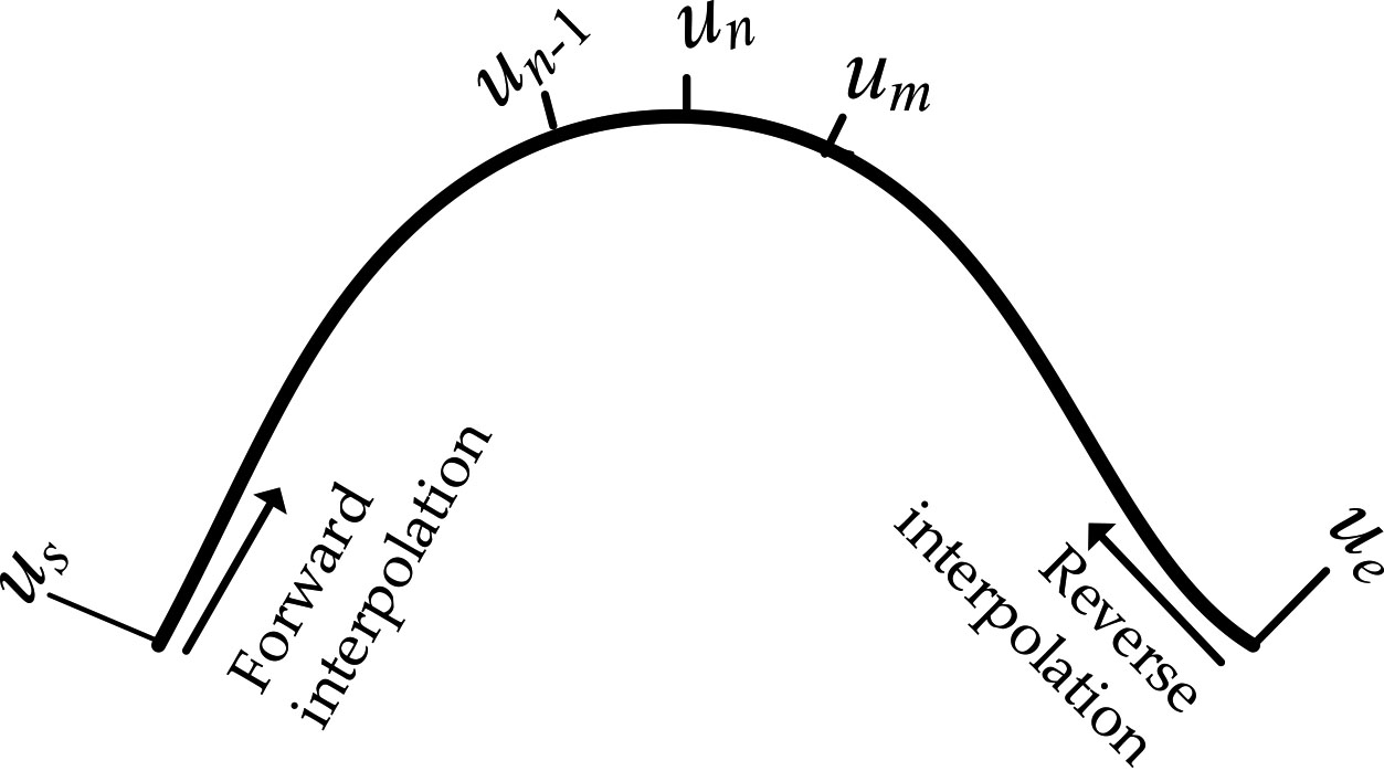

To verify the effectiveness of the presented NURBS interpolation method, simulations are conducted on an Intel Core i7-8565U 1.8 GHz personal computer, and MATLAB 7.0 and 1.8 GHz dualcore CPU computers are used for the simulation. The experiment is divided into two groups: 1). a fast pre-interpolation experiment (FPIM) that we proposed, with maximum binary exponential orders of 5, 8, 10, 12 and 15 for five comparative experiments and 2). a bidirectional acceleration and deceleration experiment using the S-shaped acceleration and deceleration method to implement speed planning for a curve segment The adaptive feedrate interpolation (AFI) is adopted for comparison [24]. In the simulation, the interpolation period $T$ is set to 2 ms, and the command feedrate is set to $F=$ 0.2 mm/ms. The maximum chord error is set to $\delta_{\max}=$ 0.001 mm, and the maximum allowable tangential acceleration and tangential acceleration of the machine tool are $10^{-3}$ mm/ms ${}^{2}$ and $10^{-4}$ mm/ms ${}^{3}$ , respectively. In the simulation experiment, the NURBS curve is selected as the interpolation curve, that is, the tool path (as shown in Fig. 4), and the curve parameters are shown in Table 1. The curvature distribution of the NURBS curve is shown in Fig. 5. Smooth curvature regions and abrupt curvature regions are present.

Figure 4.

An 8-shaped NURBS curve.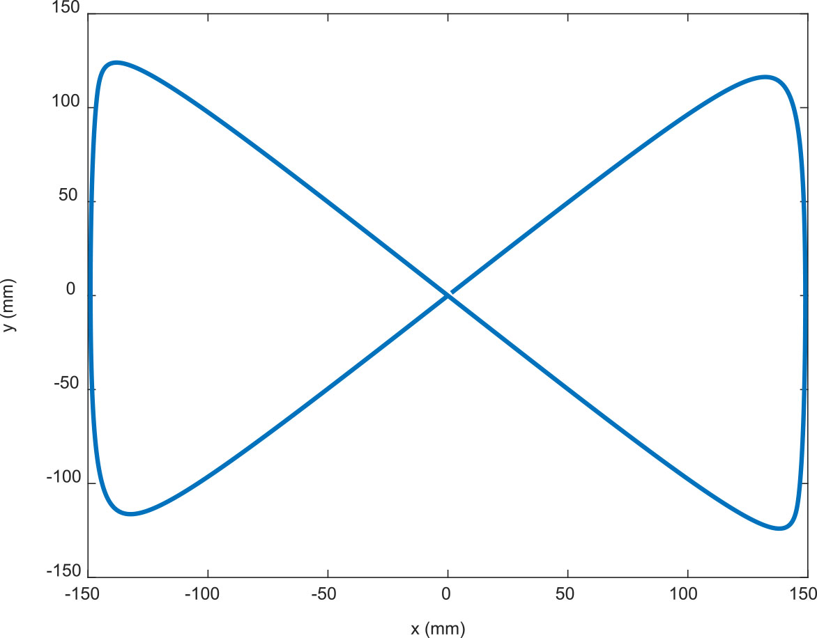

Figure 5.

Curvature of the 8-shaped NURBS curve.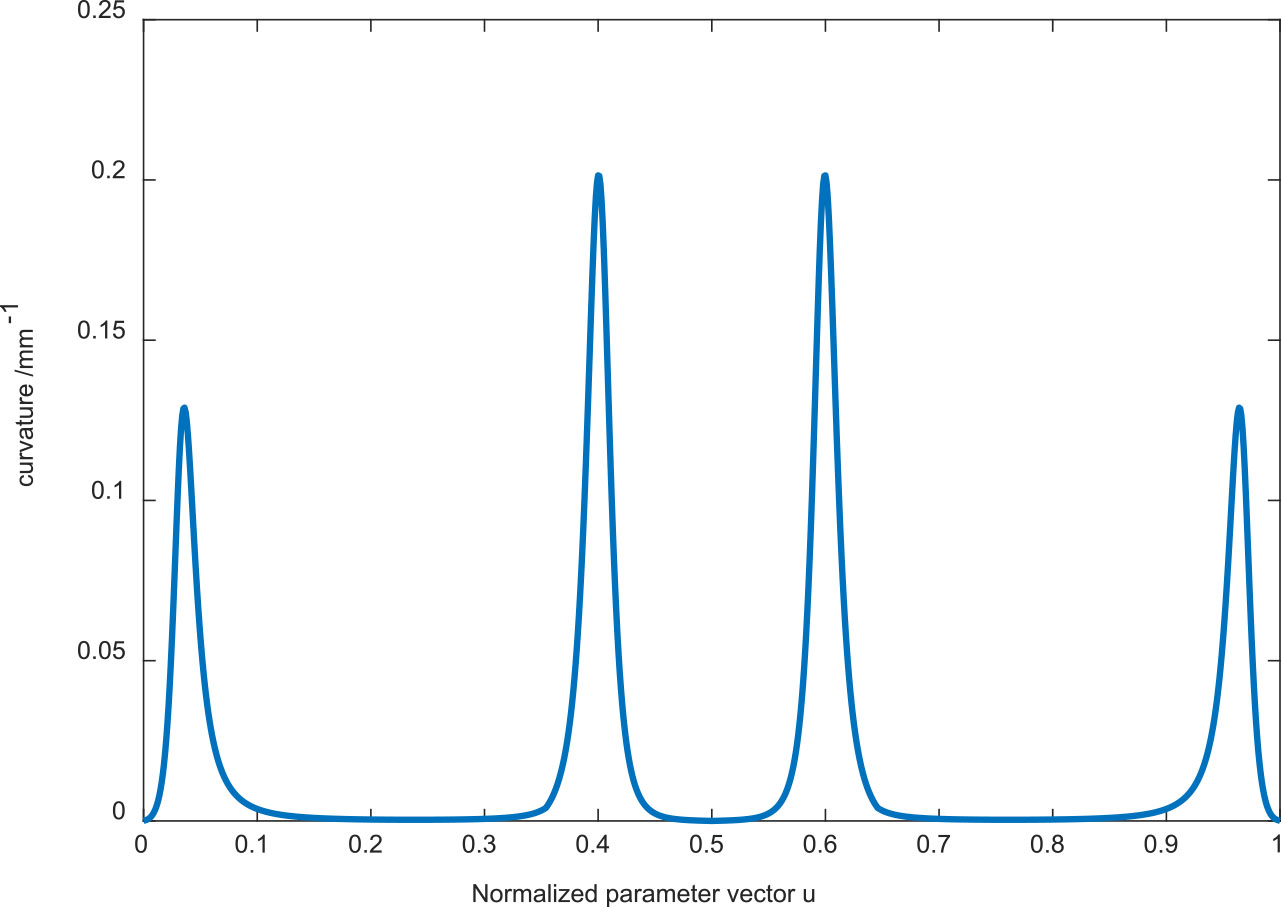

Table 2 compares fast pre-interpolation of different orders. At the same time, the first-order Taylor expansion approximation method is used as the reference. The table shows that the larger the order is, the fewer the number of interpolation points that will be generated; in contrast, the smaller the order is, the greater the number of feedrate sensitive areas that will be missed. For example, when the order value is 5, the effect is not as good as that of the first-order Taylor expansion approximation; when the value is 15, two feedrate sensitive areas will be missed.

From the perspective of effectiveness, the first-order Taylor expansion method, FPMI (order 5, 8, 10, 12) is valid, shown as T in the Table 2, while FPMI (order 15) is invalid, shown in the Table 2 is F because two velocity-sensitive regions are omitted. It can be seen from this that the choice of order is the key to FPMI, and optimization algorithms such as ant colony algorithm and simulated annealing can be used to optimize this value, which will not be repeated here due to space limitations.The interpolation points produced by fast pre-interpolation are significantly reduced compared with that of the first-order Taylor expansion approximation when the appropriate order value is used, and the real-time performance of our method is substantially improved compared with that of the first-order Taylor approximation.

Table 2

Comparison of different orders using fast pre-interpolation methods (FPIM)

Method	Number of points	Number of sensitive areas	Take the first-order Taylor expansion as a contrast	Effectiveness
First-order Taylor expansion	3130	4	100%	T
Order 5(FPIM)	3462	4	110.6%	T
Order 8(FPIM)	610	4	19.5%	T
Order 10(FPIM)	364	4	11.6%	T
Order 12(FPIM)	292	4	9.3%	T
Order 15(FPIM)	151	2	4.8%	F

Figure 6.

Feedrate profile of the eight-shaped NURBS curve by AFI.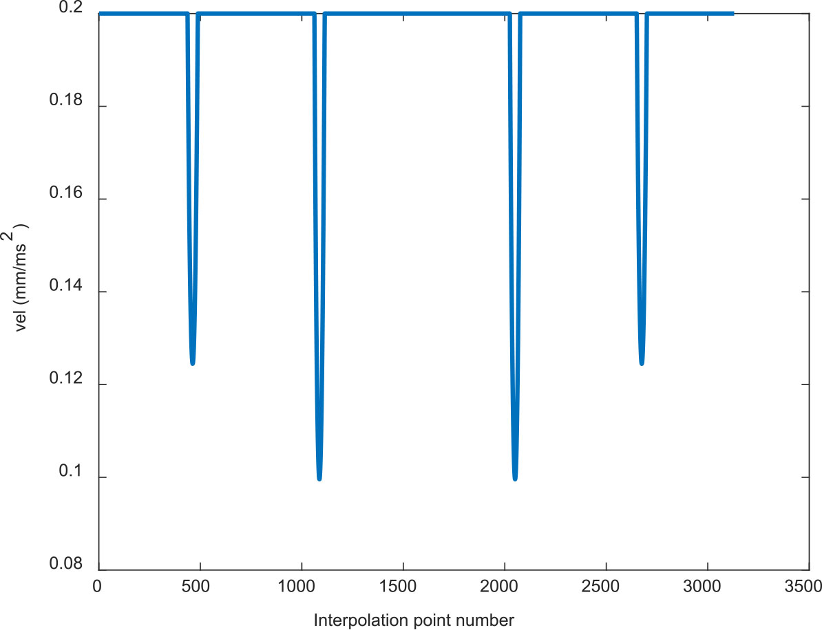

Figure 7.

Feedrate profile of the eight-shaped NURBS curve by 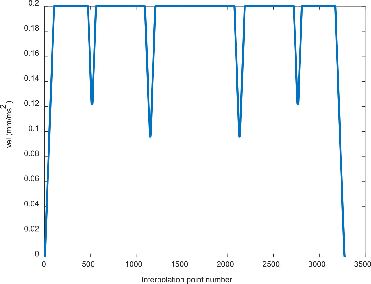FPIM.

Figure 8.

ACC profile of the eight-shaped NURBS curve by AFI.

The feedrate profiles of the eight-shaped NURBS curve by the two methods are shown in Figs 6 and 7, and the corresponding acceleration and jerk profiles are presented in Figs 8–11, respectively. As shown in Fig. 6, the initial speed of the feedrate profile begins and ends with the maximum command speed, which leads to a large vibration and severely affects the processing quality. During the feedrate adaptive adjustment, the feedrate limit is only based on the maximum chord error in the AFI method. As a result, the tangential acceleration of the AFI method, as shown in Fig. 8, exceeds the maximum allowable range and cannot meet the limit conditions. The same is true for the tangential acceleration, as shown in Fig. 10. The maximum absolute value of the tangential acceleration is 0.004383 mm/s ${}^{2}$ by AFI as shown in Fig. 10, which is more than sevenfold the maximum allowable value. The maximum absolute value of the tangential jerk is 0.002051 mm/s ${}^{3}$ by AFI as shown in Table 3, which is more than 20-fold the maximum allowable value.

Figure 9.

ACC profile of the eight-shaped NURBS curve by 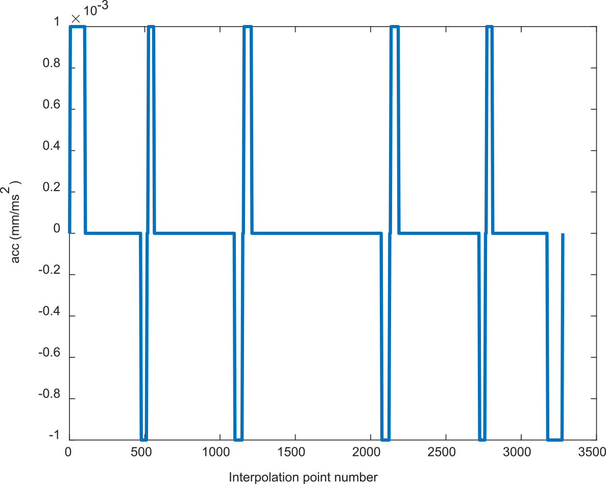FPIM.

Figure 10.

Jerk profile of the eight-shaped NURBS curve by AFI.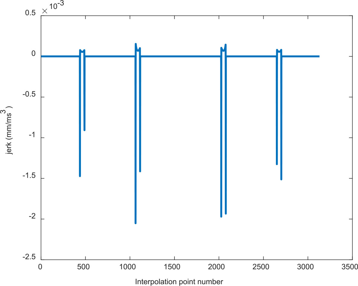

Compared with the AFI method, the FPIM method has more advantages. As shown in Fig. 7, the initial speed of the feedrate profile begins and ends at zero, which is consistent with the characteristics of the S-type acceleration and deceleration method. The FPIM method obtains a smooth feedrate profile and meets the limits of chord error, normal acceleration and normal jerk because of the two-way speed planning algorithm combined with S-curve acceleration and deceleration planning. Therefore, from Figs 9 and 11, the tangential acceleration and tangential jerk by the FPIM method can be kept within the limits so that the tangential acceleration meets the maximum acceleration tolerance to avoid the feedrate abrupt fluctuation, as shown in Table 3. The tangential jerk falls into the range of [ $-1\times 10^{-4}mm/ms^{3},1\times 10^{-4}mm/ms^{3}$ ], which can make acceleration smooth and prevent vibration to the machine tool. Thus, we can conclude that throughout the interpolation process, the acceleration is always controlled within the maximum allowable value, indicating that no sudden change in acceleration occurs during the interpolation process.

Table 3

Comparison of the simulation results of the two methods

Method	Start/end speed	Maximum acceleration fluctuation	Maximum jerk fluctuation
AFI	2 mm/ms	438%	2051%
FPIM (proposed)	0 mm/ms	100%	100%

Figure 11.

Jerk profile of the eight-shaped NURBS curve by FPIM.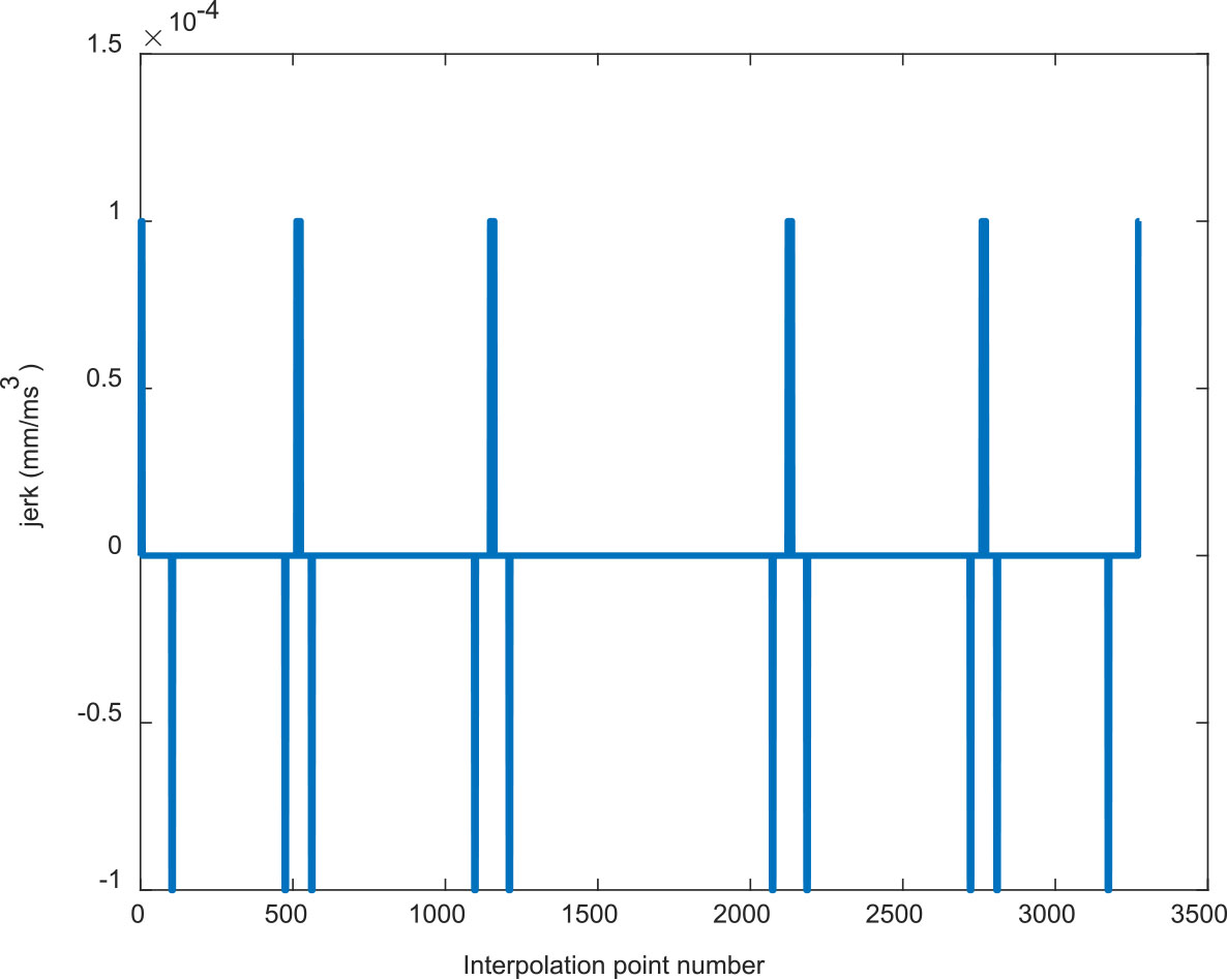

According to the simulation results, the advantages of the proposed method compared with the traditional method are list as follows: 1) The proposed method can reduce the number of pre-interpolation points by 80–90% compared with the first-order Taylor expansion method. 2) The proposed method can always meet the tolerance requirements at the maximum acceleration and maximum jerk, while the maximum acceleration fluctuation and maximum jerk fluctuation of the traditional AFI method reach 438% and 2051%, respectively. Therefore, the proposed method has a great improvement, which can achieve high-speed and high-precision interpolation.

7. Conclusion

In this paper, a look-ahead interpolation method is proposed based on an exponential function with offline feedrate optimization. According to the simulation results, the proposed method has better performance than the traditional method in terms of the number of pre-interpolation points and speed stability. The next step will continue to study the optimization method for step size parameter selection, implementing fast NURBS interpolation techniques.

Footnotes

Acknowledgments

This work is supported by the Natural Science Foundation of Hunan Province under Grant No. 2021JJ30574 and is partly supported by the Research Foundation of Education Bureau of Hunan Province under Grant No. 21B0424.

References

Baek

Yang

. Fast and precision NURBS interpolator for CNC systems. Int J Precis Eng Manuf. 2012; 13: 955-961.

Erwinski

Paprocki

Karasek

. Comparison of NURBS trajectory interpolation algorithms for high-speed motion control systems. 2021 IEEE 19th International Power Electronics and Motion Control Conference (PEMC). IEEE, 2021.

Obukhov

Martinova

Lyubimov

. Developing of the Look Ahead Algorithm for Linear and Nonlinear Laws of Control of Feedrate in CNC. Automation and Remote Control. 2020; 81(2): 380-386.

Liu

Huang

Yin

Guo

Shao

Zhang

. Development and implementation of a NURBS interpolator with smooth feedrate scheduling for CNC machine tools. International Journal of Machine Tools and Manufacture. 2014; 87: 1-15.

Shpitalni

Koren

. Realtime curve interpolators. Computer-Aided Design. 1994; 26(11): 832-8.

Yeh

Hsu

. Adaptive-feedrate interpolation for parametric curves with a confined chord error. Computer-Aided Design. 2002; 34(3): 229-37.

Tikhon

Lee

Kim

. NURBS interpolator for constant material removal rate in open NC machine tools. International Journal of Machine Tools and Manufacture. 2004; 44(2): 237-45.

Park

Nam

Yang

. Development of a real-time trajectory generator for NURBS interpolation based on the two-stage interpolation method. International Journal of Advanced Manufacturing Technology. 2005; 26(4): 359-65.

Tsai

Cheng

Lin

Tsai

. On acceleration/deceleration before interpolation for CNC motion control. In: Proceedings of IEEE International Conference on Mechatronics. 2005; pp. 382-7.

10.

Yong

Narayanaswami

. A parametric interpolator with confined chord errors, acceleration and deceleration for NC machining. CAD Comput. Aided Des. 2003; 35(13); 1249-1259.

11.

Sencer

Altintas

Croft

. Feed optimization for five-axis CNC machine tools with drive constraints. Int J Mach Tools Manuf. 2008; 48(7-8); 733-745.

12.

Nam

Yang

. A study on a generalized parametric interpolator with real-time jerk-limited acceleration, CAD Comput. Aided Des. 2004; 36(1): 27-36.

13.

Annoni

Bardine

Campanelli

Foglia

Prete

. A real-time configurable NURBS interpolator with bounded acceleration, jerk and chord error. Comput. Aided Des. 2012; 44: 509-521.

14.

Beudaert

Lavernhe

Tournier

. Feedrate interpolation with axis jerk constraints on 5-axis NURBS and G1 tool path. Int J Mach Tools Manuf. Jun. 2012; 57; 73-82.

15.

Nam

Yang

. A study on a generalized parametric interpolator with real-time jerk-limited acceleration. Computer-Aided Design. 2004; 36(1): 27-36.

16.

Jahanpour

Alizadeh

. A novel acc-jerk-limited NURBS interpolation enhanced with an optimized S-shaped quintic feedrate scheduling scheme. International Journal of Advanced Manufacturing Technology. 2014; 77(9-12): 1889-1905.

17.

Jia

Song

. A NURBS interpolator with constant speed at feedrate-sensitive regions under drive and contour-error constraints. International Journal of Machine Tools & Manufacture: Design, Research and Application, 2017.

18.

Liu

Yuan

. Adaptive feedrate planning on parametric tool path with geometric and kinematic constraints for CNC machining. The International Journal of Advanced Manufacturing Technology, 2017.

19.

Erkorkmaz

Chen

Zhao

Beudaert

Gao

. Linear programming and windowing based feedrate optimization for spline toolpaths. CIRP Ann. 2017; 66: 393-396.

20.

Wang

T-Y

Zhang

Y-B

Dong

J-C

R-J

Ding

Y-Y

. NURBS Interpolator with Adaptive Smooth Feedrate Scheduling and Minimal Feedrate Fluctuation. International Journal of Precision Engineering and Manufacturing. 2020; 21(2): 273-290.

21.

Chen

Sun

. Contour error-bounded parametric interpolator with minimum feedrate fluctuation for five-axis CNC machine tools. International Journal of Advanced Manufacturing Technology, 2019.

22.

Zhong

Luo

Chang

, etc. A real-time interpolator for parametric curves. International Journal of Machine Tools & Manufacture: Design, research and application, 2018.

23.

Zhang

Shi

, et al. Development of an Adaptive-Feedrate Planning and Iterative Interpolator for Parametric Toolpath with Normal Jerk Constraint. International Journal of Precision Engineering and Manufacturing. 2020; 22(1).

24.

Yuan

, et al. Feedrate Scheduling of NURBS Interpolation Based on A Novel Jerk-continuous ACC/DEC Algorithm. IEEE Access, 2018: 1-1.

Development of look-ahead NURBS interpolation based on the exponential function

Abstract

Keywords

1. Introduction

2. The concept of interpolation of the NURBS curve

4.1 Fast pre-interpolation

Table 1 The parameters of NURBS curve

Footnotes

Acknowledgments

References

Table 1
The parameters of NURBS curve