A noise resistant dependency measure for rough set-based feature selection

Abstract

The aim of feature selection (FS) is to select a small subset of most important and discriminative features. Many FS approaches based on rough set theory up to now, have employed reduct analysis using feature dependency measures. However the critical shortcoming for such approaches is that they are not able to manage useful information that may be destroyed by noise elements. Therefore several extensions to the original theory have been proposed. Three notable extensions are fuzzy rough set (FRS), variable precision rough set (VPRS), and tolerance rough set model (TRSM). Although successful, each of the extensions exhibits a critical shortcoming which makes that extension inapplicable in most of scenarios. For example, FRS is able to describe the existing dependencies between different attributes accurately, but its high run-times makes it inapplicable to larger datasets. As another example, VPR is very fast, but requires more information than contained within the data itself, which is inaccessible for most of the applications. This paper examines a rough set FS technique which uses a noise resistant dependency measure to quantify information that may be hidden due to the noise elements. Experimental results demonstrate that the use of this measure can result more discriminative reducts than those obtained using other RSFS approaches. Moreover, the proposed measure is as fast as VPRS and as accurate as FRS and TRSM, while it need no additional information other than contained within the data.

Keywords

Feature selection rough sets theory impurity measure noise resistant dependency

1 Introduction

Although larger feature set gives more information about a concept, we need to keep the feature set as small as possible to reduce computational complexity, gain good generalization performance and increase accuracy [9, 30]. In the feature selection problems, a set of feature vectors with n input features and one or more output features, is given and the task is to select a small subset of most important and discriminative input features.

On feature selection, a specific theoretical framework is Pawlak’s rough set model [25]. This model tries to express vagueness by means of positive and boundary regions of a set. The main advantage of this theory is that it requires no human input or domain knowledge other than the given data set [24]. This property makes the rough sets a powerful mathematical tool for analyzing various types of data [4 , 35].

Most existing classical rough-set-based feature selection (RSFS) approaches [10 , 36] rely on reduct analysis. A reduct is a sufficient subset of input features that fully characterizes the positive region structure generated by the full feature set. Although successful, these positive region-based approaches has three shortcomings which make them ineffective in real world applications; Firstly, they only operate effectively with datasets containing discrete values and therefore it is necessary to perform a discretization step for real-valued attributes. Secondly, these methods examine only the information contained within the lower approximation of a set and ignore the information contained in the boundary region. Finally, These methods are highly sensitive to noisy data and useful information that may be destroyed by noise elements are all ignored by classical RSFS methods [15 , 24].

Motivated by these shortcomings, several extensions to the original theory have been proposed. This extensions can be divided into two categories:

Extensions which focus on the modification of the equivalence relation, such as tolerance rough sets model (TRSM) [28] and fuzzy rough sets (FRS) [6, 15]. TRSM uses a similarity relation instead of indiscernibility relation to relax the crisp manner of classical rough sets theory. FRS, on the other hand, uses fuzzy equivalence classes generated by a fuzzy similarity relation to represent vagueness in data. While these extensions are able to handle the classical rough set shortcomings, they needs considerable computational time to apply their modifications. Therefore these extensions are not computationally efficient in large datasets.

Extensions which consider manipulation of the subset operator used in calculating rough set approximations. The notable extension in this group is variable precision rough sets (VPRS) [37]. VPRS attempts to overcome the classical rough set shortcomings by generalizing the standard set inclusion relation. While this extension is fast, it requires more information than contained within the data itself. This is contrary to the rough sets theory consideration of operating with no domain knowledge.

In addition to rough sets extensions, there are also some classical rough set based feature selection approaches which consider the boundary region information. In [12, 18] the upper approximations are examined instead of lower approximations, to define feature selection criterions. The approach proposed in [24] examines both the information in the lower approximation and the information contained in the boundary region for the selection of feature subsets. While all this methods are successful in dealing with real-valued datasets and using information contained in the boundary region, they are not designed to deal with noisy datasets. Noise is an integral part of many real world datasets, which could hide important information about the output features. This paper presents a method which can handle noisy data. The proposed method uses a set impurity measure to quantify information that may be hidden due to the noise elements. This measure combined with the proximity measure adopted in [24], constitute a noise resistant dependency measure which enables the RSFS approaches to deal with real-valued datasets, use information contained in the boundary region and control possible noise elements.

In summary, the unique contributions that distinguish the proposed work from existing approaches are threefold: 1) Our work advances the classical RSFS one step further for handling noisy data; 2) a novel feature selection criterion is proposed which needs no human input or domain knowledge; and 3) a new feature selection algorithm is proposed, with extensive comparisons and experimental studies to prove its accuracy and speed.

The remainder of the paper is organized as follows: Section 2 summarizes the theoretical background of RSFS along with a look at the rough set extensions and QUICKREDUCT algorithm. Section 3 presents the main contribution of the new approach with a description of the noise resistant measure for RSFS. Section 4 reports experimental results and Section 6 concludes the paper.

2 Rough sets

The rough sets theory is introduced by Pawlak [25] to express vagueness by means of boundary region of a set. The main advantage of this implementation of vagueness is that it requires no human input or domain knowledge other than the given data set [24, 31, 24, 31]. This section describes the fundamentals of thetheory.

2.1 Information system and indiscernibility

An information system is a pair IS = (U, F), where U is a non-empty finite set of objects called universe and F is a non-empty finite set of features such that f : U → V_f, for every f ∈ F. The set V_f is called the value set or domain of f. Information system in rough sets theory is analogous with data set in unsupervised machine learning and classification tasks. A decision system is an information system of the form IS = (U, F, d), where d is called the decision feature. data set in a supervised classification and learning can be seen as a decision system, where instances are the objects of universe, features are the elements of F and labels represent decision feature values.

For any set B ⊆ F ∪ {d}, we define the B-indiscernibility relation as: $\begin{matrix} {IND}_{IS} (B) \\ = {(x, y) \in U \times U | \forall f \in B, f (x) = f (y)} \end{matrix}$ (1)

If (x, y) belongs to IND_IS (B), x and y are indiscernible according to the feature subset B. Equivalence classes of the relation IND_IS (B) are denoted [x] _B and referred to as B-elementary sets. The partitioning of U to B-elementary subsets is denoted U/IND_IS (B) or simply U/B. Generating such a partitioning is a common computational routine, that effects the performance of any rough set based operation. Algorithm 1 represents a general procedure PARTITION to compute U/B.

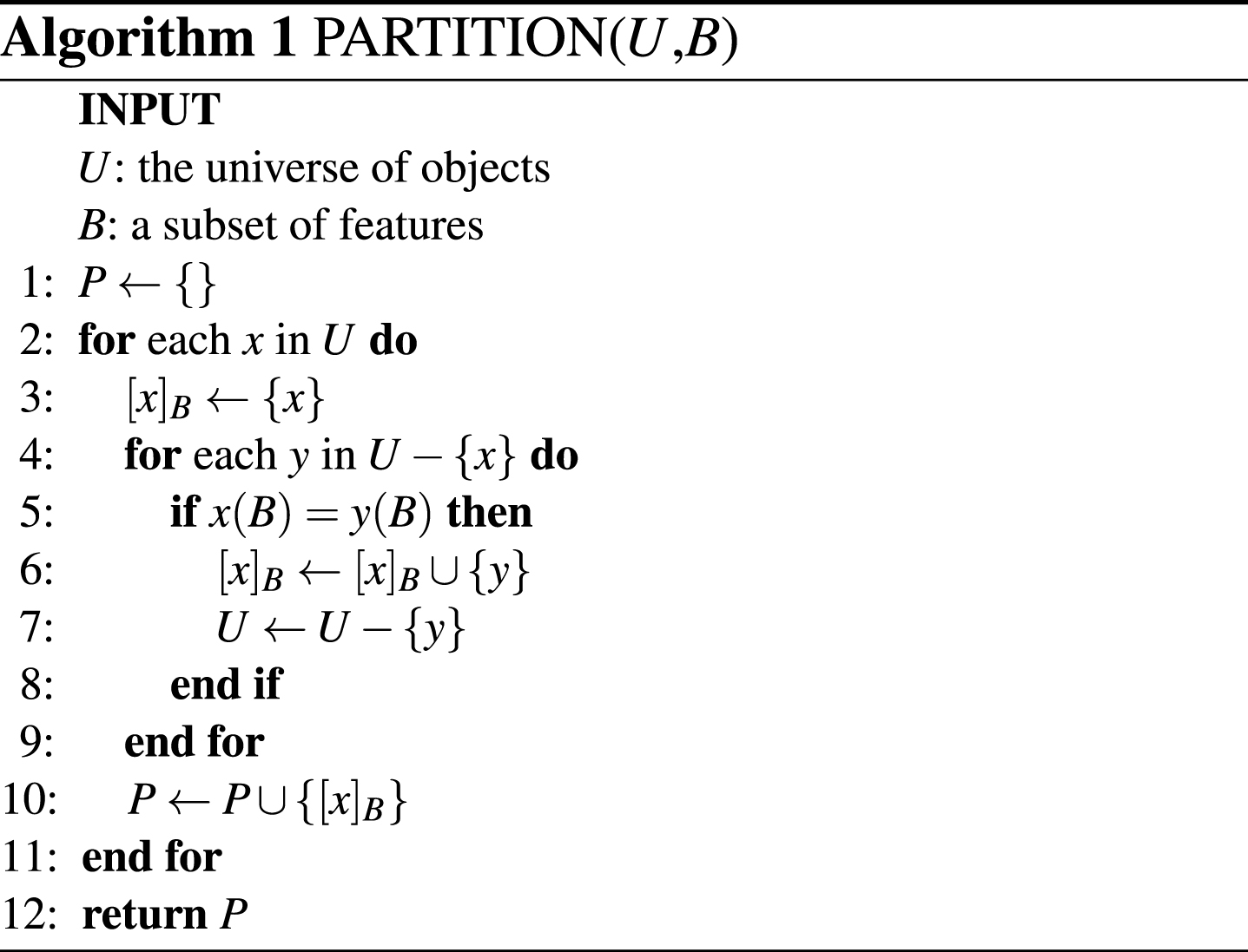
The time complexity of PARTITION is Θ (|B||P||U|), where |P| is the number of generated B-elementary subsets. If none of the objects in U are indiscernible according to B, the number of B-elementary subsets is |U| and therefore the worst-case complexity of PARTITION is O (|B||U|²).

2.2 Lower and upper approximations

The fundamental notions of rough sets are lower and upper approximations of sets. let B ⊆ F and X ⊆ U, the B-lower and B-upper approximations of X are defined as follow: $\underline{B} X = {x | [x]_{B} \subseteq X}$ (2) $\bar{B} X = {x | [x]_{B} \cap X \neq 0}$ (3)

The $\underline{B} X$ and $\bar{B} X$ approximations define information contained in B [24]. If $x \in \underline{B} X$ , it is certain that it belongs to X and if $x \in \bar{B} X$ , we can only say that x may belong to X.

By the definition of $\underline{B} X$ and $\bar{B} X$ , the objects in U can be partition into three regions which are the positive, boundary and negative regions. ${POS}_{B} (X) = \underline{B} X$ (4) ${BND}_{B} (X) = \bar{B} X - \underline{B} X$ (5) ${NEG}_{B} (X) = U - \bar{B} X$ (6)

While all the patterns in the positive region could be certainly included in the set, the boundary region consists of those patterns that can neither be ruled in nor ruled out as members of the set. Moreover, all the patterns in the negative region could be certainly excluded from the set.

2.3 Dependency

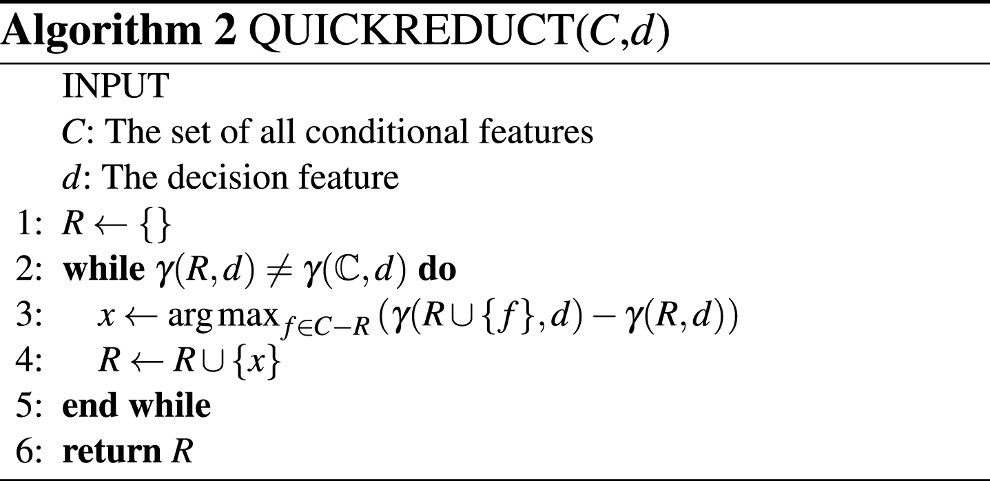
Discovering dependencies between attributes is an important issue in data analysis. Let D and C be subsets of F ∪ {d}. It is said that D depends on C in a degree k (0 ≤ k ≤ 1), denoted C ⇒ _kD, if $k = γ (C, D) = \frac{| {POS}_{C} (D) |}{| U |}$ (7) where ${POS}_{C} (D) = ⋃_{X \in U / D} \underline{C} X$ called a positive region of the partition U/D with respect to C. This region is the set of all elements of U that can be uniquely classified to blocks of the partition U/D, by means of C [29]. Functional dependency of D and C denoted C ⇒ D is an special case of dependency where γ (C, D) =1. In this case we say that all values of attributes from D are uniquely determined by values of attributes from C.

2.4 Reduct

A reduct R is a minimal set of features R ⊆ C, such that γ (R, d) = γ (C, d) [15, 17]. An optimal reduct is a reduct with minimum cardinality. Finding a minimal reduct is NP-hard [15], because all the possible subsets of conditional features must be generated to retrieve such a reduct. Therefore finding a near optimal reduct has generated much of interest [14 , 17]. Figure 2 represents the steps of QUICKREDUCT algorithm [14], which searches for a minimal subset without exhaustively generating all possiblesubsets.

2.5 Rough set extensions

Several efforts has been made to make close the attribute reduction concept in rough sets theory and feature selection in machine learning and classification tasks. However traditional rough set based attribute reduction (RSAR) has three shortcomings which make it ineffective in real world applications [15 , 24]; First, it only operates effectively with datasets containing discrete values and therefore it is necessary to perform a discretization step for real-valued attributes. Second, RSAR is highly sensitive to noisy data. Finally, RSAR methods examine only the information contained within the lower approximation of a set and ignore the information contained in the boundary region.

Therefore several extensions to the original theory have been proposed to overcome such shortcomings. Four notable extensions are variable precision rough sets (VPRS) [37], tolerance rough set model (TRSM) [28], fuzzy rough sets (FRS) [6, 15] and an extension to dependency measure proposed in [24].

VPRS [37] attempts to overcome the traditional rough sets shortcomings by generalizing the standard set inclusion relation (⊆). In the generalized inclusion relation, a set X is considered to be a subset of Y if the proportion of elements in X which are not in Y is less than a predefined threshold. However, the introduction of a suitable threshold requires more information than contained within the data itself. This is contrary to the rough sets theory consideration of operating with no domain knowledge.

TRSM [28] uses a similarity relation instead of indiscernibility relation to relax the crisp manner of classical rough sets theory. As equivalence classes (elementary sets) in classical rough sets, tolerance classes are generated using similarity relation in TRSM, which are used to define lower and upper approximations. TRSM has two deficiencies; First, it needs a tolerance threshold to generate tolerance classes, which like VPRS this threshold is human defined. Second, the time complexity of generating all tolerance classes, using attribute subset B, is Θ (|B||U|²), which is equal to worst-case time complexity of PARTITION algorithm.

FRS [6, 15] uses fuzzy equivalence classes generated by a fuzzy similarity relation to represent vagueness in data. Fuzzy Lower and upper approximations are generated based on fuzzy equivalence classes. These approximations are extended versions of their crisp notions in classical rough sets, except that in the fuzzy approximations, elements may have membership degree in the range [0, 1]. FRS needs no extra knowledge to define operations on a given dataset, however as tolerance classes in TRSM, generating fuzzy equivalence classes in FRS is an expensive routine (Θ (|B||U|²)).

In addition to rough sets extensions, there are also some modifications, which does not change classical rough sets principals. [24] redefines the dependency notion in classical rough sets to deal with useful information that may be contained in the boundary region. Unlike the other three extensions, this extension does not redefine the lower and upper approximations in classical rough sets, therefore it needs no human input knowledge to deal with available data. Moreover the PARTITION algorithm may be applied directly, that is, generating equivalence classes in this extension is more efficient that generating tolerance classes and fuzzy equivalence classes in TRSM and FRS, respectively. Since this extension has been used as a part of our work, it is explained more extensive in the following subsection.

2.5.1 Useful information in the boundary region

Almost all the classical rough set based attribute reduction methods use only the information contained in the positive region. However the boundary region may also contain useful information that are ignored in this methods [24]. Such scenario is common in real-valued datasets, where some adjacent values may placed in different regions because of crisp manner of classical rough sets. Measuring the proximity of objects in the boundary region to the objects in positive region could help to qualify the information contained in boundary region. The method proposed in [24] uses a distance metric to calculate such proximities.

Let X be a set of objects and B a subset of attributes. The mean positive region, which is the mean of all object attribute values in POS_B (X), is defined as $m = {\frac{\sum_{x \in \underline{B} X} f (x)}{| {POS}_{B} (X) |} : \forall f \in B}$ (8)

The proximity of any object y ∈ BND_B (X) from the mean positive region is defined as $δ_{B} (m, y) = {\begin{matrix} d (m, y) & if | {POS}_{B} (X) | \neq 0 \\ 0 & if | {POS}_{B} (X) | = 0 \end{matrix}$ (9) where d can be any distance function such as euclidean distance metric.

The proximity of the boundary region to the positive region is defined as $ω (C, D) = {\begin{matrix} ψ_{B}^{- 1} & if | {BND}_{C} (D) | \neq 0 \\ 1 & if | {BND}_{C} (D) | = 0 \end{matrix}$ (10) where $ψ_{B} = \sum_{y \in {BND}_{B} (X)} δ_{B} (m, y)$ (11)

This proximity measure combined with rough-set dependency value create a new evaluation measure M as $M (C, D) = \frac{γ (C, D) + ω (C, D)}{2}$ (12)

The DMQUICKREDUCT (distance metric assisted QUICKREDUCT), a version of QUICKREDUCT that uses the new measure to guide the attribute reduction process, is presented in Algorithm 3.

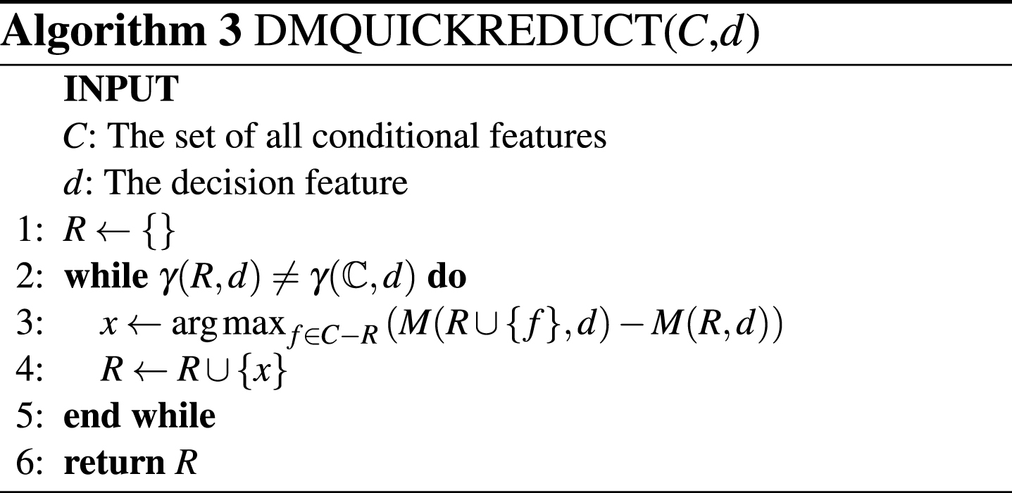
It is important to point out that the value of M is used as an attribute selection criterion, not as a termination criterion. At each iteration, the algorithm adds a conditional feature that causes maximum increase in the value of M for the selected subset. The algorithm terminates when the dependency value of selected subset (γ (R, d)) reaches that of the unreduced data set.

3 Attribute reduction using noise resistant dependency measure

Using classical dependency combined with proximity of boundary and positive regions enables the attribute reduction algorithm to deal with real-valued datasets. However this measure is insufficient to control noisy data, specially in non real-valued datasets. For example suppose two binary attributes a and b (Table 1), where a is 0 for all first half instances and 1 for all second half and b is similar to a, except that a value from first half is exchanged with a value from second half. Obviously b is a noisy version of a. Let C = {a} and D = {b} then $U / C = {{1, 2, 3, 4}, {5, 6, 7, 8}}$ and $U / D = {{1, 2, 3, 8}, {4, 5, 6, 7}}$ then ${POS}_{C} (D) = ⋃ {\underline{C} {1, 2, 3, 8}, \underline{C} {4, 5, 6, 7}} = \emptyset$

Therefore γ (C, D) =0 based on (7), which implies that the two attribute sets are independent from the classical rough sets view point. Moreover they have no dependency even if we use (12), because ω (C, D) =0 based on (10).

Table 1
An example table

x ∈ U a b

1 0 0

2 0 0

3 0 0

4 0 1

5 1 1

6 1 1

7 1 1

8 1 0

x ∈ U	a	b
1	0	0
2	0	0
3	0	0
4	0	1
5	1	1
6	1	1
7	1	1
8	1	0

The problem comes from the crisp manner of the inclusion relation in defining lower approximations. Suppose for example the case $\underline{C} {1, 2, 3, 8}$ in calculating POS_C (D). This approximation is an empty set, because non of the elementary sets in U/C are a subset of {1, 2, 3, 8}. However suppose the elementary set {1, 2, 3, 4} in U/C. If we remove 4 (the noise element) from this subset, the positive region will not be empty any more. The same rule can be applied to {5, 6, 7, 8}, removing 8 (another noise element). This example can simply extended for more than two attributes.

The approach described in this section uses a noise resistant dependency measure to search for reducts. The NRRSAR method uses the information that may be hidden due to noise elements and assigns a significance value to this information.

3.1 Impurity rate and noise resistant measure

The noise resistant measure attempts to qualify the information that may be unseen due to the crisp manner of the inclusion relation in defining lower approximations. This measure uses an impurity rate value to calculate the noisy portion of a set. Let A and B be two sets. The impurity rate of A with respect to B can be defined as follow: $c (A, B) = \frac{| A - B |}{| A |}$ (13)

This value calculates the portion of the elements that should be eliminated from A to make it totally included in B. It is important to note that if c (A, B) >0.5, the impurity of A with respect to B is more than its impurity with respect to $\bar{B}$ . In this case, A could be supposed as a noisy version of $\bar{B}$ and all elements in A ∩ B will constitute the noisy portion of A. Therefore, the B-related information that could be retrieved after removing impurities from A can be formulated as $ξ (A, B) = {\begin{matrix} 1 - c (A, B) & if c (A, B) \leq 0.5 \\ 0 & if c (A, B) > 0.5 \end{matrix}$ (14)

This formulation can be applied to elementary sets to extract information that may be unseen in calculating lower approximations. To do this, a noise measure function, φ, is defined as $φ_{B} (X) = \frac{\sum_{Y \in U / B} ξ (Y, X) [ξ (Y, X) \neq 1]}{| U / B |}$ (15)

This function quantifies the possibility of transferring some objects from boundary to the positive region of a set, if the noisy elements could be removed.

Let C and D be two attribute sets. The noisy dependency of D on C can be defined as follow: $ν (C, D) = \sum_{X \in U / D} φ_{C} (X)$ (16)

Suppose the example in Table 1. The noisy dependency of D = {b} on C = {a} can be calculated as $\begin{matrix} ν (C, D) & = & φ_{C} ({1, 2, 3, 8}) + φ_{C} ({4, 5, 6, 7}) \\ = & \frac{ξ ({1, 2, 3, 4}, {1, 2, 3, 8})}{2} \\ + \frac{ξ ({5, 6, 7, 8}, {1, 2, 3, 8})}{2} \\ + \frac{ξ ({1, 2, 3, 4}, {4, 5, 6, 7})}{2} \\ + \frac{ξ ({5, 6, 7, 8}, {4, 5, 6, 7})}{2} \\ = & \frac{\frac{3}{4} + 0}{2} + \frac{0 + \frac{3}{4}}{2} = 0.75 \end{matrix}$

The noisy dependency operates on boundary region as proximity measure (10). However the proximity measure considers each point in the boundary region separately and calculates its distance from the positive region, while the noisy dependency considers subsets of objects to measure their transmission possibility to the positive region. Therefore the two values are combined to create a new measure for evaluating boundary region as $τ (C, D) = \frac{ω (C, D) + ν (C, D)}{2}$ (17)

This new measure can be used alongside the classical dependency. As one measure only operates on the objects in boundary region and the other only on the objects in positive region, the two operators are combined to create a noise resistant evaluation measure ρ: $ρ (C, D) = \frac{τ (C, D) + γ (C, D)}{2}$ (18)

For the example in Table 1, $ρ (C, D) = \frac{\frac{0 + 0.75}{2} + 0}{2} = 0.1875$

3.2 Noise resistant attribute reduction

The proposed noise resistant measure can be used as an attribute selection criterion in rough set based attribute reduction algorithms. Algorithm 4 shows NRQUICKREDUCT algorithm, which is similar to QUICKREDUCT and DMQUICKREDUCT algorithms, but uses the proposed measure to guide the attribute reduction process.

The algorithm starts with an empty selected attribute set R. At each iteration, an attribute is added to R from non-selected attributes. This attribute is selected such that its addition causes maximum increase in the value of the noise resistant measure. This process continues until the dependency value of the selected attributes (γ (R, d)) equals the dependency of complete conditional attribute set (γ (C, d)). It is important to point out that as DMQUICKREDUCT, the new measure is used as an attribute selection criterion, not as a termination criterion.

4 Experimental results

In this section, we provide several experimental results to illustrate the performance of the proposed measure. To do this, NRRSAR is compared with two types of algorithms 1) classical rough set-based attribute reduction algorithms, and 2) attribute reduction algorithms based on rough sets extensions. Results are presented in terms of the selected subset size (compactness), the time to locate the subset (run-time) in seconds, the classification accuracy and the robustness against different types of noises.

Table 2 summarizes the 13 data sets, used in our experiments. The data sets range from 6 to 100 attributes, and 32 to 4177 objects. The monk3, abalone, tic-tac-toe, wine, credit, zoo, dermatology, ionosphere, soybean-small, heart, and lung-cancer datasets are from the UCI machine learning repository [1] and the tm1, and tm2, two synthetic problems called threshold max, are from [26]. If available, we have used the original test set as evaluating dataset, and for the remaining data sets, 10-fold cross-validation is used.

Table 2
Summary of the Benchmark Datasets (C: categorical, R: real-valued, I: integer)

No. Dataset # Attributes # Train # Test Type

1 monk3 6 122 C

2 abalone 8 4177 C, I, R

3 tic-tac-toe 9 958 C

4 wine 13 178 I, R

5 credit 15 690 C, I, R

6 zoo 17 101 C, I

7 dermatology 33 366 C, I

8 ionosphere 34 351 I, R

9 soybean-small 35 47 C

10 heart 44 267 I

11 lung-cancer 56 32 I

12 tm1 100 1000 R

13 tm2 100 1000 R

No.	Dataset	# Attributes	# Train	Type
1	monk3	6	122	C
2	abalone	8	4177	C, I, R
3	tic-tac-toe	9	958	C
4	wine	13	178	I, R
5	credit	15	690	C, I, R
6	zoo	17	101	C, I
7	dermatology	33	366	C, I
8	ionosphere	34	351	I, R
9	soybean-small	35	47	C
10	heart	44	267	I
11	lung-cancer	56	32	I
12	tm1	100	1000	R
13	tm2	100	1000	R

All the experiments are carried out on a DELL workstation with Windows 7, 2 GB memory, and 2.4 GHz CPU. Four classifiers are employed for the classification of the data, J48 [27, 33], JRip [3], Naive Bayes [5], and kernel SVM with RBF kernel function [2]. To set the classifier-related parameters, such as the C and γ parameters of the kernel SVM, we used the 5-fold cross validation.

4.1 Comparison of NRRSAR with RSAR and DMRSAR

Here, the performance of the proposed measure, is compared with RSAR and DMRSAR [24]. In this regard, NRQUICKREDUCT algorithm is compared with QUICKREDUCT and DMQUICKREDUCT algorithms.

Table 3, report the selected subset sizes found by the three measures. As it can be seen, RSAR found smaller results in comparison to both DMRSAR and NRRSAR. This is reasonable, since the termination criterion and the objectives are the same in QUICKREDUCT iterations, while the DMQUICKREDUCT and NRQUICKREDUCT algorithms may find features, which do not necessarily increase the dependency function value (the stopping criterion). While the result obtained by NRRSAR is larger than that obtained by DMRSAR for dermatology, DMRSAR found subsets which are close to the original feature set in 2 cases (ionosphere and lung-cancer). This is an important result which demonstrates the unreliability of adopting DMRSAR on real valued data sets. Table 3 reports the compactness of the selected subsets using the three SBE algorithms on the large scale data sets. We can conclude that SBE-NRRSAR selects fewer features than the other two algorithms.

Table 3
Comparison of Selected Subsets Size for RSAR, DMRSAR and NRRSAR

Dataset RSAR DMRSAR NRRSAR

monk3 4 4 4

abalone 4 6 4

tic-tac-toe 8 8 8

wine 2 2 2

credit 3 3 3

zoo 5 5 5

dermatology 7 7 9

ionosphere 3 20 4

soybean-small 2 2 2

heart 5 6 5

lung-cancer 5 41 10

tm1 5 19 8

tm2 5 21 8

Dataset	RSAR	DMRSAR	NRRSAR
monk3	4	4	4
abalone	4	6	4
tic-tac-toe	8	8	8
wine	2	2	2
credit	3	3	3
zoo	5	5	5
dermatology	7	7	9
ionosphere	3	20	4
soybean-small	2	2	2
heart	5	6	5
lung-cancer	5	41	10
tm1	5	19	8
tm2	5	21	8

Table 4 reports the run-times of the three measures on small scale data sets. It is clear that the selected subset size affects the run-times, but considering those tests with equal selected subset sizes enables us to make a clear comparison between the methods. Comparing with RSAR and DMRSAR, the results show that there is only a marginal increase in runtime for the NRRSAR iterations. This means that, there is little overall difference in runtime between the proposed noise resistant dependency measure and the other two measures.

Table 4

Comparison of Run Times for RSAR, DMRSAR and NRRSAR

Dataset	RSAR	DMRSAR	NRRSAR	0.21	0.27	0.34
abalone	111.43	203.22	149.32
tic-tac-toe	10.58	13.35	14.35
wine	1.33	2.16	2.73
credit	14.09	18.39	21.65
zoo	6.93	7.41	8.02
dermatology	21.61	24.96	30.04
ionosphere	12.03	98.59	19.22
soybean-small	0.17	0.22	0.27
heart	17.92	21.87	21.78
lung-cancer	1.02	18.17	5.01
tm1	423.32	2372.83	881.9
tm2	412.82	2711.62	872.92

Table 5 reports the classification results. As it can be seen, the proposed NRRSAR based algorithm (NRQUICKREDUCT) performs very well and shows increase in classification accuracies for most of the tests.

Table 5

Comparison of Classification Results for RSAR, DMRSAR and NRRSAR, Using J48, JRip, Naive Bayes (NB), and SVM

Dataset	RSAR				DMRSAR				NRRSAR
	J48	JRip	NB	SVM	J48	JRip	NB	SVM	J48	JRip	NB	SVM
monk3	98.11	93.95	96.44	98.11	98.11	93.95	96.44	98.11	98.11	93.95	96.44	98.11
abalone	68.12	59.84	65.29	77.96	34.02	32.74	40.88	38.13	92.10	90.00	94.65	99.02
tic-tac-toe	82.50	90.62	88.41	90.62	82.50	90.62	88.41	90.62	86.02	98.94	88.94	96.18
wine	80.20	81.66	88.88	89.30	80.20	81.66	88.88	89.30	85.13	82.05	86.24	86.24
credit	55.10	58.00	69.21	58.00	55.10	58.00	69.21	58.00	87.42	86.33	92.43	94.86
zoo	93.05	90.18	90.18	92.66	93.05	90.18	90.18	92.66	93.05	92.66	94.00	90.18
dermatology	79.45	80.00	73.81	78.18	78.53	78.12	76.04	77.99	79.59	81.5	80.00	80.17
ionosphere	63.84	84.30	71.08	87.75	74.20	84.30	68.11	75.93	76.29	88.59	77.50	92.92
soybean-small	76.82	78.44	48.13	80.51	76.82	78.44	48.13	80.51	89.67	88.36	85.10	86.12
heart	80.95	81.29	76.74	75.50	79.59	76.10	64.84	76.10	82.11	81.29	76.00	75.50
lung-cancer	32.06	39.74	38.00	40.55	88.63	88.63	46.17	58.91	90.50	89.33	72.10	88.36
tm1	85.10	91.25	88.19	91.25	62.30	48.26	62.70	62.70	95.05	95.05	92.70	95.05
tm2	94.22	96.16	96.84	95.39	66.20	68.11	49.23	58.92	98.00	98.00	96.84	98.00

Compared with RSAR (QUICKREDUCT) in terms of J48 classifier, the NRRSAR is superior in all tests. Moreover, NRRSAR shows an increase of up to 60 percent for lung-cancer and up to 30 percent for credit. Comparing the two algorithms in terms of JRip, we see the similar results to those discussed for J48. Using Naive Bayes, the RSAR shows slightly better results for the wine and heart datasets, but we can see that our proposed algorithm is superior in the other eleven datasets and it shows an increase of up to 40 percent for lung-cancer, up to 35 percent for soybean-small and lung-cancer, and up to 30 percent for abalone datasets. In terms of SVM classifier, NRRSAR lost the tests only for two cases wine and zoo, while it shows significant increases in classification results for most of the remaining tests.

Compared with DMRSAR (DMQUICKRED-UCT) in terms of J48, our proposed algorithm is superior in all tests and shows an increase of up to 55 percent for abalone, and up to 30 percent for credit, tm1 and tm2. Using JRip, NRRSAR is superior in all tests and we can see that this algorithm shows an increase of up to 55 percent for abalone, up to 45 percent for tm1 and up to 30 percent for credit and tm2. Although NRRSAR lost the test for wine in terms of Naive Bayes classifier, it shows an increase of up to 55 percent for abalone and up to 45 percent for tm2. Using SVM, we can see the similar results to those discussed for JRip. Using SVM, the DMRSAR shows slightly better results for three data sets wine, zoo and heart, but we can see that our proposed algorithm shows significant increases for ninecases.

4.2 Comparison of NRRSAR with rough set extensions

Here, the performance of the proposed measure, is compared with three rough set extensions, VPRS, TRSM, and FRS.

4.2.1 Comparison with VPRS

To compare the proposed measure with VPRS, NRQUICKREDUCT is compared with a QUICKREDUCT algorithm witch employs the VPRS-based dependency function as feature selection criterion. In our experiments two different threshold values β = 0.1 and β = 0.2 are employed to define the generalized inclusion relation in VPRS-based algorithm.

Table 6 reports the selected subsets size and run times. Comparing with NRRSAR, VPRS found smaller subsets for some tests, however the results show a strong dependence of this method on the β-value. Although the ideal threshold value can be obtained by repeated experimentation for a given data set, this value will be biased to the used data set. Moreover, finding such a value will impose a large computational time to the overall feature selection process. There are few tests with equal selected subsets for NRRSAR and VPRS, but considering those few tests demonstrate that the two methods are comparable in terms of run-times for small scale data sets.

Table 6
Comparison of Selected Subsets Size and Run Times for NRRSAR and VPRS

Dataset Selected Subset Size Run Time

NRRSAR VPRS NRRSAR VPRS

β = 0.1 β = 0.2 β = 0.1 β = 0.2

monk3 4 6 3 0.34 2.35 0.66

abalone 4 4 4 149.32 170.38 167.48

tic-tac-toe 8 8 9 14.35 12.70 13.05

wine 2 2 2 2.73 2.65 2.22

credit 3 3 3 21.65 17.87 17.91

zoo 5 6 4 8.02 9.93 6.04

dermatology 9 7 7 30.04 40.51 29.58

ionosphere 4 2 1 19.22 10.98 4.82

soybean-small 2 2 2 0.27 0.32 0.32

heart 10 5 6 21.78 23.99 32.18

lung-cancer 10 5 5 5.01 2.87 1.65

tm1 8 19 16 881.9 2384.33 1659.03

tm2 8 18 13 872.92 2008.28 1422.88

Dataset	Selected Subset Size	Run Time
monk3	4	6	3	0.34	2.35	0.66
abalone	4	4	4	149.32	170.38	167.48
tic-tac-toe	8	8	9	14.35	12.70	13.05
wine	2	2	2	2.73	2.65	2.22
credit	3	3	3	21.65	17.87	17.91
zoo	5	6	4	8.02	9.93	6.04
dermatology	9	7	7	30.04	40.51	29.58
ionosphere	4	2	1	19.22	10.98	4.82
soybean-small	2	2	2	0.27	0.32	0.32
heart	10	5	6	21.78	23.99	32.18
lung-cancer	10	5	5	5.01	2.87	1.65
tm1	8	19	16	881.9	2384.33	1659.03
tm2	8	18	13	872.92	2008.28	1422.88

Table 7 reports the classification results using NRRSAR and VPRS. As it can be seen, NRQUICKREDUCT shows increases in classification accuracies for most of the tests. In terms of J48 classifier, NRQUICKREDUCT is superior for at least one β setting. Moreover this algorithm is superior in eleven cases considering both β settings. The proposed algorithm won the tests for ten, nine and eleven data sets using JRip, Naive Bayes and SVM classifiers, respectively.

Table 7

Comparison of Classification Results for NRRSAR and VPRS, Using J48, JRip, Naive Bayes (NB), and SVM

Dataset	NRRSAR				VPRS
					β = 0.1				β = 0.2
	J48	JRip	NB	SVM	J48	JRip	NB	SVM	J48	JRip	NB	SVM
monk3	98.11	93.95	96.44	98.11	97.22	94.73	96.00	90.44	83.49	81.36	88.99	86.13
abalone	92.10	90.00	94.65	99.02	88.20	88.20	91.72	92.00	87.22	84.29	91.70	94.88
tic-tac-toe	86.02	98.94	88.94	96.18	84.71	91.29	82.02	92.66	84.01	93.01	88.05	90.49
wine	85.13	82.05	86.24	86.24	84.23	82.92	88.50	90.24	84.23	82.92	88.50	90.24
credit	87.42	86.33	92.43	94.86	55.80	53.28	46.00	51.12	55.80	53.28	46.00	51.12
zoo	93.05	92.66	94.00	90.18	90.12	88.29	82.45	85.14	89.99	90.15	88.02	88.02
dermatology	79.59	81.5	80.00	80.17	58.27	59.17	58.66	60.33	89.12	90.10	66.23	78.10
ionosphere	76.29	88.59	77.50	92.92	63.81	88.59	64.10	63.81	63.81	89.02	74.39	80.20
soybean-small	89.67	88.36	85.10	86.12	76.34	77.92	64.18	72.58	76.34	77.80	81.26	79.60
heart	82.11	81.29	76.00	75.50	80.74	59.22	54.18	78.03	85.33	88.11	90.01	93.19
lung-cancer	90.50	89.33	72.10	88.36	71.58	47.84	69.12	68.66	73.33	68.08	68.44	72.18
tm1	95.05	95.05	92.70	95.05	34.82	41.10	36.00	49.02	52.94	60.17	36.01	40.73
tm2	98.00	98.00	96.84	98.00	61.90	72.83	64.55	65.51	52.99	59.82	52.99	58.85

4.2.2 Comparison with TRSM and FRS

TRSM [28] and FRS [6, 15] try to relax the crisp manner of the classical rough set theory by modifying the equivalence relation. TRSM uses a similarity relation instead of indiscernibility relation to define such a relaxation. FRS, on the other hand, uses fuzzy equivalence classes generated by a fuzzy similarity relation to represent vagueness in data.

Although different similarity measures can be adopted in TRSM, we have used a standard measure for this purpose given in [28]: $S_{f} (x, y) = 1 - \frac{| f (x) - f (y) |}{| \max (f) - \min (f) |}$ (19)

When the objects have more than one feature, the similarity relation is defined as: $(x, y) \in S_{P, α} \Leftrightarrow \frac{\sum_{f \in P} S_{f} (x, y)}{| P |} \geq α$ (20)

Where P is the feature set and α is a predefined threshold. In our experiments, two different values of tolerance thresholds α = 0.9 and α = 0.95 are used for TRSM.

Generating all tolerance classes in TRSM as well as fuzzy equivalence classes in FRS is quadratic with respect to the number of objects, because, the similarities of all pairs of objects must be calculated. These complexity burdens cause high computational times for TRSM and FRS, even for small scale data sets. Therefore, the comparisons in this subsection are reported only for eight data sets monk3, wine, zoo, dermatology, ionosphere, soybean-small, heart, and lung-cancer. In this regard, NRQUICKREDUCT is compared with a TRSM-based and FRS-based QUICKREDUCT algorithms.

Table 8 reports the selected subsets size and run times for the eight data sets. Similar to VPRS, the optimal threshold value in TRSM is data driven and needs a pre-processing step for each data set. This is contrary to the rough sets theory consideration of operating with no domain knowledge. The results show that NRRSAR outperforms the FRS for two data sets (ionosphere and lung-cancer), while the two methods found same size subsets for the remaining tests. High computational times of FRS and TRSM, is the most prominent result from this table.

Table 8

Comparison of Selected Subsets Size for NRRSAR, TRSM, and FRS

	Selected Subset Size				Run Time
Dataset	NRRSAR	TRSM		FRS	NRRSAR	TRSM		FRS
		α = 0.9	α = 0.95			α = 0.9	α = 0.95
monk3	4	4	4	4	0.34	2.81	2.87	6.92
wine	2	4	3	2	2.73	212.09	154.41	712.18
zoo	5	5	5	5	8.02	109.92	113.90	300.19
dermatology	9	9	9	9	30.04	795.05	840.46	1448.39
ionosphere	4	6	7	6	19.22	551.56	683.09	1278.11
soybean-small	2	2	2	2	0.27	2.00	2.00	5.01
heart	10	6	6	9	21.78	771.26	796.02	1927.83
lung-cancer	10	5	5	13	5.01	33.25	33.24	86.19

4.3 Statistical evaluation

In order to strengthen the comparisons, we used a paired hypothesis t-test. Let A and B be two methods and d_A, d_B be the set of results obtained using methods A and B, respectively, for different executions. We define the following two one-tailed t-tests [7]: $t 1 : {\begin{matrix} H_{0} : μ_{d_{A}} = μ_{d_{B}} \\ H_{1} : μ_{d_{A}} > μ_{d_{B}} \end{matrix}$ (21) $t 2 : {\begin{matrix} H_{0} : μ_{d_{A}} = μ_{d_{B}} \\ H_{1} : μ_{d_{B}} > μ_{d_{A}} \end{matrix}$ (22) where, μ_D is the population mean of set D.

Based on results of these tests, the variable t is defined as $t = {\begin{matrix} ↑ & if the null hypothesis (H_{0}) in t_{1} is rejected \\ ↓ & if the null hypothesis in t_{2} is rejected \\ = & if H_{0} is not rejected in both t_{1} and t_{2} \end{matrix}$ (23)

In all the tests, A corresponds to our proposed NRRSAR method and B corresponds to one of the five methods RSAR, DMRSAR, VPRS, TRSM and FRS. The results are reported in Table 10.

Table 9

Comparison of Classification Results for NRRSAR, TRSM and FRS, Using J48, JRip, Naive Bayes (NB), and SVM

Dataset	NRRSAR				TRSM								FRS
				β = 0.1				β = 0.2
	J48	JRip	NB	SVM	J48	JRip	NB	SVM	J48	JRip	NB	SVM	J48	JRip	NB	SVM
monk3	98.11	93.95	96.44	98.11	98.11	93.95	96.44	98.11	78.20	82.64	84.35	72.25	98.11	93.95	96.44	98.11
wine	85.13	82.05	86.24	86.24	83.95	75.30	75.30	75.82	84.11	78.32	80.46	83.19	89.67	88.36	85.10	86.12
zoo	93.05	92.66	94.00	90.18	93.05	92.66	94.00	90.18	93.05	92.66	94.00	90.18	93.05	92.66	94.00	90.18
dermatology	79.59	81.5	80.00	80.17	79.59	81.5	80.00	80.17	79.59	81.5	80.00	80.17	79.59	81.5	80.00	80.17
ionosphere	76.29	88.59	77.50	92.92	76.29	88.59	77.50	92.92	76.29	88.59	77.50	92.92	76.29	88.59	77.50	92.92
soybean-small	89.67	88.36	85.10	86.12	89.67	88.36	85.10	86.12	89.67	88.36	85.10	86.12	89.67	88.36	85.10	86.12
heart	82.11	81.29	76.00	75.50	74.84	74.84	79.50	74.84	74.84	74.84	79.50	74.84	82.11	81.29	76.00	75.50
lung-cancer	90.50	89.33	72.10	88.36	45.07	45.07	61.88	53.19	57.13	60.44	61.88	61.88	90.50	89.33	72.10	88.36

Table 10

Statistical Comparisons of NRRSAR with RSAR, DMRSAR, VPRS, TRSM and FRS

Method	Comparison Term
	Compactness	Running Time	Classification Accuracy
			J48	JRip	NB	SVM
RSAR	↑	↑	↑	↑	↑	↑
DMRSAR	↓	=	↑	↑	↑	↑
VPRS	=	=	↑	↑	↑	↑
TRSM	=	↓	=	=	=	=
FRS	=	↓	=	=	=	=

4.4 Robustness against noise

Here, we investigate the effect(s) of noise on selected subsets of different attribute reduction algorithms. In this regard, several levels of noises are added to the datasets and then the six feature selection algorithms are applied again on these datasets. In order to add a noise with probability K to a decision system D = (U, F, d), we changed f_i (x) , i = 1, 2, …, |F|, x = 1, 2, …, |U|, with probability K, as follows

If f_i is categorical or integer-valued feature, with value set (domain) V_{f
_i}, then we replaced f_i (x) with a randomly selected value from V_{f
_i} - {f_i (x)}.

If f_i is a real-valued feature, then we first normalized f_i (x) using the following formula: $f_{i}^{(n)} (x) = \frac{f_{i} (x) - \min (f_{i})}{\max (f_{i}) - \min (f_{i})}$ (24) Then we added a noise to $f_{i}^{(n)} (x)$ as $g_{i} (x) = f_{i}^{(n)} (x) + N (0, α)$ (25) where α is a value selected randomly from [0, 0.5] and $N (0, α)$ is a gaussian noise with mean 0 and variance α. Finally we re-scaled g_i (x) using the following formula: $f_{i} (x) = g_{i} (x) (\max (f_{i}) - \min (f_{i})) + \min (f_{i})$ (26)

For each algorithm A and decision system D, we define two functions $Θ_{A}^{D}$ and $Δ_{A}^{D}$ as $Θ_{A}^{D} = | \frac{R_{A}^{(D)} \cap R_{A}^{(D^{(n)})}}{R_{A}^{(D)}} |$ (27) $Δ_{A}^{D} = | \frac{R_{A}^{(D^{(n)})} - R_{A}^{(D)}}{R_{A}^{(D^{(n)})}} |$ (28)

Where,

A: an attribute reduction algorithm,

D⁽ⁿ⁾: the decision system D which is disrupted using noise,

$R_{A}^{(D)}$ : the set of selected features using algorithm A for decision system D.

$Θ_{A}^{D} \in [0, 1]$ is a measure of how much algorithm A is able to select those features for D⁽ⁿ⁾, which are selected for D. Moreover, $Δ_{A}^{D} \in [0, 1]$ is a measure of how much algorithm A selects features for D⁽ⁿ⁾, which are not selected for D.

For each data set, we generated 30 disrupted versions by different settings for K (the noise probability). Then, we applied the comparing feature selection algorithms on the original data sets and their corresponding disrupted versions. For each disrupted version, we recorded the Θ and Δ measures.

Tables 11 and 12 report the Θ and Δ values, respectively, recorded for the comparing algorithms. The results for each algorithm and data set are averaged over the 30 executions. As it can be seen from these tables, noises have least effect on results of the proposed NRRSAR algorithm, while the other algorithms are very noise-sensitive and their results are destroyed, even using small levels of noises.

Table 11

Θ Results Recorded for NRRSAR, RSAR, DMRSAR, VPRS, TRSM and FRS

Dataset	NRRSAR	RSAR		DMRSAR		VPRS				TRSM				FRS
						β = 0.1		β = 0.2		α = 0.9		α = 0.95
		avg	t	avg	t	avg	t	avg	t	avg	t	avg	t	avg	t
monk3	0.94	0.39	↑	0.43	↑	0.49	↑	0.45	↑	0.71	↑	0.70	↑	0.71	↑
abalone	0.86	0.33	↑	0.36	↑	0.51	↑	0.53	↑	-	-	-	-	-	-
tic-tac-toe	0.89	0.48	↑	0.47	↑	0.52	↑	0.52	↑	-	-	-	-	-	-
wine	0.99	0.72	↑	0.84	↑	0.84	↑	0.82	↑	0.90	↑	0.86	↑	0.93	↑
credit	0.91	0.37	↑	0.39	↑	0.48	↑	0.48	↑	-	-	-	-	-	-
zoo	0.99	0.67	↑	0.73	↑	0.79	↑	0.78	↑	0.88	↑	0.89	↑	0.89	↑
dermatology	0.86	0.51	↑	0.49	↑	0.57	↑	0.62	↑	0.67	↑	0.54	↑	0.64	↑
ionosphere	0.90	0.47	↑	0.63	↑	0.61	↑	0.57	↑	0.62	↑	0.68	↑	0.73	↑
soybean-small	1	0.92	↑	0.93	↑	0.75	↑	0.84	↑	0.93	↑	0.89	↑	0.92	↑
heart	0.88	0.61	↑	0.56	↑	0.71	↑	0.80	↑	0.78	↑	0.77	↑	0.79	↑
lung-cancer	0.97	0.74	↑	0.80	↑	0.79	↑	0.78	↑	0.82	↑	0.85	↑	0.87	↑
tm1	0.90	0.52	↑	0.71	↑	0.64	↑	0.67	↑	-	-	-	-	-	-
tm2	0.95	0.55	↑	0.53	↑	0.59	↑	0.51	↑	-	-	-	-	-	-

Table 12

Δ Results Recorded for NRRSAR, RSAR, DMRSAR, VPRS, TRSM and FRS

Dataset	NRRSAR	RSAR		DMRSAR		VPRS				TRSM				FRS
						β = 0.1		β = 0.2		α = 0.9		α = 0.95
		avg	t	avg	t	avg	t	avg	t	avg	t	avg	t	avg	t
monk3	0.12	0.64	↓	0.48	↓	0.53	↓	0.57	↓	0.28	↓	0.28	↓	0.31	↓
abalone	0.15	0.71	↓	0.64	↓	0.52	↓	0.50	↓	-	-	-	-	-	-
tic-tac-toe	0.10	0.53	↓	0.54	↓	0.46	↓	0.49	↓	-	-	-	-	-	-
wine	0.01	0.30	↓	0.16	↓	0.16	↓	0.18	↓	0.09	↓	0.15	↓	0.08	↓
credit	0.10	0.64	↓	0.63	↓	0.51	↓	0.55	↓	-	-	-	-	-	-
zoo	0.00	0.33	↓	0.30	↓	0.22	↓	0.78	↓	0.12	↓	0.12	↓	0.12	↓
dermatology	0.16	0.51	↓	0.53	↓	0.45	↓	0.38	↓	0.35	↓	0.45	↓	0.38	↓
ionosphere	0.09	0.53	↓	0.39	↓	0.38	↓	0.47	↓	0.38	↓	0.37	↓	0.28	↓
soybean-small	0.00	0.08	↓	0.07	↓	0.31	↓	0.15	↓	0.08	↓	0.12	↓	0.09	↓
heart	0.13	0.42	↓	0.45	↓	0.32	↓	0.19	↓	0.26	↓	0.22	↓	0.23	↓
lung-cancer	0.03	0.28	↓	0.19	↓	0.19	↓	0.22	↓	0.17	↓	0.16	↓	0.13	↓
tm1	0.11	0.53	↓	0.34	↓	0.40	↓	0.35	↓	-	-	-	-	-	-
tm2	0.07	0.51	↓	0.49	↓	0.45	↓	0.46	↓	-	-	-	-	-	-

5 Conclusions

Feature selection, as a pre-processing step, is to select a small subset of most important and discriminative input features. This paper investigated a new feature selection method, NRRSAR, which aims to meet the existing RS based feature selection methods of dealing with noisy data sets. In the experiments, our study has shown that, NRRSAR outperforms the existing RS based feature selection methods, RSAR and DMRSAR, in terms of classification accuracies. Moreover, the results show that there is only a marginal increase in runtime for the NRRSAR iterations, comparing it with RSAR andDMRSAR.

Comparison with a VPRS-based feature selection method has demonstrated that while this method may sometimes find smaller subsets, it requires an additional threshold value, which makes it an unreliable method for real world data sets. NRRSAR requires no such human input knowledge and relies only on the information in the data. Moreover, NRRSAR is able to find subsets with higher classification accuracies than those obtained by VPRS. Comparison of NRRSAR with a TRSM-based feature selection method has shown that the NRRSAR method is able to outperform TRSM in terms of classification accuracy and run times. In addition, as VPRS, the requirement to a thresholding value is a big disadvantage for the TRSM-based feature selection. Comparison with a FRS-based feature selection method has demonstrated that, while NRRSAR is very similar to FRS in terms of selected subset size and classification accuracy, the very faster run-times of NRRSAR makes it a preferable method.

Additional comparisons have shown that noises have least effect on results of the proposed NRRSAR algorithm, while the other five algorithms are very noise-sensitive and even small levels of noises have significant effects on their results.

References

Blake

and Merz

C.J.

, UCI Repository of machine learning databases. http://www.ics.uci.edu/mlearn/MLRepository.html, 1998. [Online; accessed 06-March-2015].

Chang

C.-C.

and Lin

C.-J.

, Libsvm: A library for support vector machines, ACM Trans Intell Syst Technol 2(3) (2011), 27:1–27:27.

Cohen

W.W.

, Fast effective rule induction. In Proceedings of the Twelfth International Conference on Machine Learning, Morgan Kaufmann, 1995, pp. 115–123.

Dai

, Rough set approach to incomplete numerical data, Information Sciences 241 (2013), 43–57.

Domingos

and Pazzani

, On the optimality of the simple bayesian classifier under zero-one loss, Machine Learning 29(2-3) (1997), 103–130.

Dubois

and Prade

, Putting rough sets and fuzzy sets together. In Słowiński

, editor, Intelligent Decision Support, volume 11 of Theory and Decision Library, Springer Netherlands, 1992, pp. 203–232.

Eskandari

and Mohammad

, Masoud, Online streaming feature selection using rough sets, International Journal of Approximate Reasoning 69 (2016), 35–57.

Greco

, Matarazzo

and Slowinski

, Rough sets theory for multicriteria decision analysis, European Journal of Operational Research 129(1) (2001), 1–47.

Guyon

and Elisseeff

, An introduction to variable and feature selection, Journal of Machine Learning Research 3 (2003), 1157–1182.

10.

Hassanien

A.E.

, Rough set approach for attribute reduction and rule generation: A case of patients with suspected breast cancer, Journal of the American Society for Information Science and Technology 55(11) (2004), 954–962.

11.

Hedar

A.R.

, Wang

and Fukushima

, Tabu search for attribute reduction in rough set theory, Soft Computing 12(9) (2008), 909–918.

12.

Inuiguchi

and Tsurumi

, Measures based on upper approximations of rough sets for analysis of attribute importance and interaction, International Journal of Innovative Computing, Information and Control 2(1) (2006), 1–12.

13.

Javidi

M.M.

and Eskandari

, Streamwise feature selection: A rough set method, International Journal of Machine Learning and Cybernetics (2016), 1–10.

14.

Jensen

and Shen

, A rough set-aided system for sorting www bookmarks. In Proceedings of the First Asia-Pacific Conference on Web Intelligence: Research and Development, WI’01, London, UK, Springer–Verlag, 2001, pp. 95–105.

15.

Jensen

and Shen

, Semantics-preserving dimensionality reduction: Rough and fuzzy-rough based approaches, IEEE Transactions on Knowledge and Data Engineering 16(16) (2004), 1457–1471.

16.

Jensen

and Shen

, Fuzzy-rough data reduction with ant colony optimization, Fuzzy Sets and Systems 149(1) (2005), 5–20.

17.

Jensen

, Tuson

and Shen

, Finding rough and fuzzy-rough set reducts with SAT, Information Sciences 255 (2014), 100–120.

18.

Jitender

H.S.

, Deogun

and Raghavan

V.V.

, Exploiting upper approximation in the rough set methodology, First Int’l Conf Knowledge Discovery and Data Mining, 1995.

19.

H.R.

and Zhang

W.X.

, Applying indiscernibility attribute sets to knowledge reduction. In AI 2005: Advances in Artificial Intelligence volume 3809, 2005, pp. 816–821.

20.

and Liu

Y.S.

, Rough set based attribute reduction approach in data mining. In Machine Learning and Cybernetics, 2002. Proceedings. 2002 International Conference on, volume 1, 2002, pp. 60–63.

21.

Liang

, Wang

, Dang

and Qian

, A group incremental approach to feature selection applying rough set technique, Knowledge and Data Engineering, IEEE Transactions on 26(2) (2014), 294–308.

22.

Liu

, Li

and Zhang

, A rough set-based incremental approach for learning knowledge in dynamic incomplete information systems, International Journal of Approximate Reasoning 55(8) (2014), 1764–1786.

23.

Modrzejewski

, Feature selection using rough sets theory. In Proceedings of the European Conference on Machine Learning, ECML ’93, London, UK, 1993, pp. 213–226.

24.

Parthaláin

N.M.

, Shen

and Jensen

, A distance measure approach to exploring the rough set boundary region for attribute reduction, Knowledge and Data Engineering, IEEE Transactions on 22(3) (2010), 305–317.

25.

Pawlak

, Rough sets, International Journal of Computer & Information Sciences 11(5) (1982), 341–356.

26.

Perkins

and Theiler

, Online feature selection using grafting. In International Conference on Machine Learning, ACM Press, 2003, pp. 592–599.

27.

Quinlan

J.R.

, C4.5: Programs for Machine Learning, Morgan Kaufmann Publishers Inc., San Francisco, CA, USA 1993.

28.

Skowron

and Stepaniuk

, Tolerance approximation spaces, Fundam Inf 27(2-3) (1996), 245–253.

29.

Swiniarski

R.W.

and Skowron

, Rough set methods in feature selection and recognition, Pattern Recognition Letters 24(6) (2003), 833–849.

30.

Theodoridis

, Koutroumbas

, Pattern Recognition, Academic Press, 2009.

31.

Walczak

and Massart

, Rough sets theory, Chemometrics and Intelligent Laboratory Systems 47(1) (1999), 1–16.

32.

Wang

and Wang

, Discovering patterns of missing data in survey databases: An application of rough sets, Expert Systems with Applications 36(3, Part 2) (2009), 6256–6260.

33.

Witten

I.H.

and Frank

, Data Mining: Practical Machine Learning Tools and Techniques, Second Edition (Morgan Kaufmann Series in Data Management Systems), Morgan Kaufmann Publishers Inc., San Francisco, CA, USA, 2005.

34.

Zhang

, Li

and Chen

, Composite rough sets for dynamic data mining, Information Sciences 257 (2014), 81–100.

35.

Zhang

, Wong

J.-S.

, Li

and Pan

, A comparison of parallel large-scale knowledge acquisition using rough set theory on different mapreduce runtime systems, International Journal of Approximate Reasoning 55(3) (2014), 896–907.

36.

Zhong

, Dong

and Ohsuga

, Using rough sets with heuristics for feature selection, Journal of Intelligent Information Systems 16(3) (2001), 199–214.

37.

Ziarko

, Variable precision rough set model, Journal of Computer and System Sciences 46(1) (1993), 39–59.

A noise resistant dependency measure for rough set-based feature selection

Abstract

Keywords

1 Introduction

2 Rough sets

2.1 Information system and indiscernibility

2.5 Rough set extensions

2.5.1 Useful information in the boundary region

Table 1 An example table x ∈ U a b 1 0 0 2 0 0 3 0 0 4 0 1 5 1 1 6 1 1 7 1 1 8 1 0

4 Experimental results

Table 3 Comparison of Selected Subsets Size for RSAR, DMRSAR and NRRSAR Dataset RSAR DMRSAR NRRSAR monk3 4 4 4 abalone 4 6 4 tic-tac-toe 8 8 8 wine 2 2 2 credit 3 3 3 zoo 5 5 5 dermatology 7 7 9 ionosphere 3 20 4 soybean-small 2 2 2 heart 5 6 5 lung-cancer 5 41 10 tm1 5 19 8 tm2 5 21 8

4.2.1 Comparison with VPRS

References

Table 1
An example table

x ∈ U a b

1 0 0

2 0 0

3 0 0

4 0 1

5 1 1

6 1 1

7 1 1

8 1 0