The research on meta-job scheduling heuristics in heterogeneous environments

3.1.1 The description of the scheduling algorithm in heterogeneous environment

In a heterogeneous environment, m processors can be used and t meta-jobs waited to be assigned. Assuming these processors and jobs are ordered, T[i] (i < i≤t) is used to indicate the i-th job, M[i] (1 < i≤m) indicates the i-th processors; Sch[i,j] is the scheduling operation, it means that the T[i] is assigned to the M[j]; ETC[i,j] (1 < i≤t,1 < j≤m) represents the accepted time of execution of Sch[i,j]; all of the ETC[i,j] compose ETC matrix; minET[i] (1 < i≤t) is the vector for the minimum time of execution; minET[i] = min (ETC[i,j]), where 1 < j≤m, indicates the minimum time of T[i] assigned to each processor (obviously this vector has t elements); RTM[j] (1 < j≤m) (ready time at machine) indicates the ready time of M[j], and this vector has m elements with each element having an initial value of 0 when Sch[i,j], RTM[j] += ETC[i,j]; MCT (minimum time of completion) matrix, MCT[i,j] = ETC[i,j] + RTM[j] (1 < i≤t,1 < j≤m), is the minimum time of completion matrix. The reason why MCT matrix is pointed out in this paper is just to illustrate problems easier, and the so-called ‘update MCT matrix’ is just the updated RTM[j]. When all jobs are scheduling, makespan = Max(RTM[j]), where 1 < j≤m.

3.1.2 The reviewing of Min-min and Max-min algorithms

The core idea of both Min-min and Max-min algorithm is to assign each job to processor with minimum completion time. However, Min-min algorithm assigns small jobs first, and Max-min assigns big ones first. Theoretically, the two should have similar abilities. Especially from the point of view of load balancing, Max-min can be more superior than Min-min. This section compares the execution of the two algorithms with two examples in order to find the reason why makespan is delayed. Example 1’s ETC matrix is shown as Tables 1 and 2 shows example 2’s ETC matrix.

In Example 1, the Min-min’s scheduling is Sch[1,1], Sch[2,2], Sch[3,1], Sch[4,2] and makespan = 114; Max-min’s scheduling is Sch[4,2], Sch[3,1], Sch[2,1], Sch[1,1] and makespan = 118. In Example 2, Min-min’s scheduling is Sch[1,1], Sch[2,2], Sch[3,1], Sch[4,2] and makespan = 147; Max-min’s scheduling is Sch[4,1], Sch[3,2], Sch[2,2], Sch[1,2] and makespan = 100. In Example 1, Min-min is optimal, and in Example 2, Max-min is better. In Table 1, job 1 has the largest difference of execution time on the two processors, and in Table 2, job 4 has the largest difference of execution time on the two processor. In Example 1, job 1 is assigned by Min-min algorithm first and Max-min last. In Example 2, job 4 is assigned by Min-min last and assigned by Max-min first. This shows that Min-min is better than Max-min in Example 1, and Max-min is better than Min-min in Example 2.

Whether it’s Max-min or Min-min, the first priority is minimal expected time of execution, However, with the algorithm goes on, the subsequent jobs will gradually deviate from the minimum execution time, and thus the overall makespan gets longer. If the jobs with bigger difference of expected time on each processors were assigned first, the sum of execution time of all jobs will be reduced, thus the degree of makespan becomes smaller, and the efficiency of algorithm will be improved. Therefore, the reason why scheduling is delayed is not as the Sufferage algorithm proposed. It is not due to the ‘suffer’ of the completion time but to the waste of the execution time (in the following content of this paper, the meaning of Sufferage is the waste of the execution time).

So, MaxD-min and MaxRD-min heuristics were pointed out.

3.1.3.1 Description of MaxD-min heuristic. In previous examples, there are two processors. The difference of execution time of a job on each processor can be calculated directly, difference = |ETC[i,1]–ETC[i,2]|. But in the case of multi-processor, the difference can’t be calculated directly. By the Probability Theory, it’s a good choice that the difference with mathematical expectation is used to replace that difference in previous examples.

Definition 1. The so-called mathematical expectation of T[i], namely Exp[i], refers to the average of the task execution time on all processors, Exp [ i ] = 1 m ∑ j = 1 m ETC [ i , j ](1)

Definition 2. The so-called ith job’s deviation of execution time, namely Dev[i], refers to the difference of Exp[i] and the job’s minimum execution time on all machines, Dev [ i ] = Exp [ i ] - min ET [ i ](2)

The main idea of MaxD-min (Max Deviation-min) heuristic is to reduce the difference of execution time and minimum execution time of each job as much as possible and thus to reduce the overall execution time of all jobs and to achieve the purpose of reduced makespan. The first step of the algorithm is similar to Min-min algorithm. The difference between them is not that the vector of minimum time of excepted execution is generated, but that the vector of deviation is. And in the second step, it is not the job with minimum execution time that is assigned like Min-min but the job with biggest deviation. In the beginning of executing MaxD-min, the job’s deviation is big, but it runs on the processor with a shorter execution time. At the end of MaxD-min, the scheduled job’s minimum execution time is close to the expectation of the job, so naturally, the job’s execution time has a probability close to minimum execution time. Thus the goal of the MaxD-min is reached. In the cases of example 1 and 2, the scheduling of MaxD-min is the same as the better of Min-min and Max-min.

3.1.3.2 MaxD-min heuristic. Input: ETC matrix;

Output: makespan(in the rest of this paper, the input and output of proposed algorithms are same)

1) forEach i, 1 < i≤t, compute Exp[i];

2) forEach i, 1 < i≤t, compute Dev[i];

3) if all jobs are assigned, then go to Step 4, otherwise

3.1) for T[i] with biggest deviation, find j(1 < j≤m), where the sum of ETC[i,j] + RTM[j] is the smallest;

3.2) Sch[i,j];

3.3) Update RTM[j],RTM[j] += ETC[i,j];

3.4) Delete this job, and go to step 3;

4) Let makespan = Max(RTM[j]),1 < j≤m;

5) return(makespan), endProgram.

3.1.3.3 Analysis of time complexity of MaxD-min. The Min-min algorithm’s time complexity is O (tm²) [2]. Compared with the Min-min, Exp[i]’s and Dev[i]’s calculation are added in MaxD-min, so 2(tm) is added, but the level of time complexity did not increase, is still O(tm²). The execution time of MaxD-min is slightly longer than the Min-min algorithm.

3.1.4.1 Description of MaxD-min heuristic. The difference with the expectation is used in MaxD-min, and it can be thought as a kind of absolute deviation, so that the relative deviation (i.e. the ratio of absolute deviation and the minimum execution time of job) also naturally became one of comparable parameters. According to the size of the relative deviation, determining the sequence of job scheduling is the core idea of MaxRD-min. The rationality of the relative deviation’s use is theoretically better than the deviation’s in the case of a large number of jobs. The experimental results are also acknowledged in this paper. The following definitions are given:

Definition 3. The so-called ith job’s relative deviation of execution time, namely ReDev[i], refers to the difference of Dev[i] and the job’s minimum execution time on all machines, ReDev = Dev [ i ] min ET [ i ](3)

In addition, in the phase of experimentation of MaxRD-min, another relative deviation is also considered, the ratio of deviation and expectation, but from the experimental results, the effect of two kinds of relative deviation’s use are similar, and this paper’s definition’s use is slightly better. In the case of Example 1, the scheduling of MaxRD-min is the same as Min-min; in the case of Example 2, the scheduling of MaxRD-min is: Sch[4,1], Sch[1,2], Sch[2,2], Sch[3,2], and makespan = 100. It has the same makespan as Max-min. In other words, the scheduling of MaxRD-min is the same as the better one between Min-min and Max-min.

3.1.4.2 MaxD-min heuristic. MaxRD-min (Max RelativeDeviation-min) heuristic is similar to MaxD-min, but minET[i] is calculated and the Dev[i] in MaxD-min is substituted by ReDev[i]. The details of MaxRD-min algorithm are as follows:

1) forEach i, 1 < i≤t, compute minET[i];

2) forEach i, 1 < i≤t, compute Exp[i];

3) forEach i, 1 < i≤t, compute ReDev[i];

4) if all jobs are assigned, then go to Step 5, otherwise;

4.1) for T[i] with biggest relative deviation, find j(1 < j≤m), where the sum of ETC[i,j] + RTM[j] is the smallest;

4.2) Sch[i,j];

4.3) Update RTM[j], RTM[j] += ETC[i,j];

4.4) Delete this job, and goto step 4;

5) Let makespan = Max(RTM[j]),1 < j≤m;

6) return(makespan), endProgram.

3.1.4.3 Analysis of time complexity of MaxRD-min The time complexity of MaxRD-min is approximate to the MaxD-min’s. The calculation of relative deviation is relatively complicated compared to that of deviation, but the time expansion are almost negligible. It’s time complexity is O(tm²) too.

MaxD-min’s and MaxRD-min’s proposed aim at the completion of the first objective of this article, i.e. to find a reliable replacement of Min-min. The replacement algorithm should have these characters: 1) simplicity and easy realization; 2) low time complexity; 3) higher efficiency than Min-min. The first two are presented in this section: MaxD-min and MaxRD-min are simple and easy to realize both and have low time complexity (the same level of time complexity with the Min-min). But the experimental proof of better efficiency of the two algorithms compared to the Min-min is still needed.

3.2.1 Idea of CA algorithm

The CA algorithm is based on the following ideas:

1) Each processors is thought as trays; 2) The time of each job running on different processors are regarded as different building blocks, the same building block will have different length on different trays; 3) Each tray just has one place that only one building block can be placed on it, if there were more building blocks, they could only be built up. So, the total execution time of all jobs on each processor will be the total height of the building blocks on the tray. The problem of scheduling algorithm focuses on the makespan was convert to: how to place these building blocks and make the tallest building blocks have a lower height than before.

If all of the combinations of building blocks were thought about, the optimal solution could be found, but it will enter a vicious circle of NP. This has no meaning for us. As the scale of the problem expands, the algorithm expands quickly into the index expanding which will cause the problem to become unsolvable. So, we should find a way to get the optimal solution quickly, and CA algorithm is such an algorithm.

The CA algorithm can be divided into two stages: 1) Place the building blocks on each tray quickly (the way they are placed should have a certain rationality); 2) This phase is the core stage of CA algorithm where we will move a building block from the tray which has the highest height of building blocks to another tray while insuring that the deviation of this move is as small as possible. Repeat 2) until each of the building block can’t be moved on the tray which has highest height of building blocks.

3.2.2 Model of the CA algorithm

The model of CA is two-tuples (Pallet, Cordwood):

Pallet is a set of trays. It has m elements and is a bijection with the set of processors in heterogeneous environments. The trays are orderly. P[i](1 < i≤m) refers to the ith tray. Each Pallet is a ternary vector (altitude, NoCoP, CoP). Altitude represents the total height of the building blocks on this tray; NoCop (number of cordwood on this pallet) is a non-negative integer representing the number of building blocks on the tray; CoP (cordwood on this pallet) represents a set of building blocks on this tray. The building blocks on each tray is orderly. CoP [j] (1≤j≤NoCoP) is the jth building block on this tray, and each CoP [j] that has two properties, [Height, Sufferage], Height is the height of CoP [j] on P[i], Sufferage is defined as:

CoP[j].Sufferage = minHeight(CoP[j]) – CoP[j]. Height, the minHeight will be defined below.

Cordwood is a set of building blocks. It has t elements and is a bijection with the set of jobs. The building blocks are considered orderly. C[i](1 < i≤m) refers to the ith blocks and each C[i] has an attributes [Height]; Height is an array that has m elements; C[i].Height[j] (1≤j≤m) represents the height of building blocks i on the tray j. It is the expected time of execution that task i is assigned to the processor j, i.e. C[i].Height[j] = ETC[i,j].

Some functions is defined on the basis of this model:

minHeight(C[i]) = min{C[i].Height[j], for each 1≤j≤m}; This function returns the minimum value of building blocks i on each tray, the value is a non-negative integer;

minSufferage(P[i].Cop[j]) = P[i].Cop[j].Sufferage; this function returns a value of the non-positive integers, and the value prefers to the minimum Sufferage due to the move of an building block from one tray to another;

nextSufferage(P[i].Cop[j]) = min{P[i].Cop[j]. Height–C[j].Height[L]≥minSufferage (P[i].Cop[j]), for each1≤L≤m And L≠I}, when P[i].Cop[j]. Sufferage is not accepted by CA, another smaller Sufferage will be found through this function, and its return value is an integer. The value will be assigned to P[i].Cop[j]. Sufferage while this function is running. If the value couldn’t be found, a special value (named sp) will be returned;

minSufferageOfP(P[i]) = min{P[i].CoP[j].Sufferage, for each 1≤j≤NoCoP And P[i].CoP[j]. Sufferage≠sp}; This function returns the smallest Sufferage of all of building blocks on P[i];

moveCordwood(i,j,CoP[L]) = (?P[i].Height > P[j] + P[i].CoP[L].Height, true, false); this function returns a Boolean value, when P[i].Height > P[j] + P[i].CoP[L].Height, the value is true, else it’s false.

In addition, an operation is defined here: MCFITJ(i,j, CoP[L]), move CoP[L] form P[i] to P[j], and update P[i] and P[j] at the same time.

3.2.3 Design of the first stage of CA algorithm

The first stage of the CA algorithm is essentially the input of the second stage, and the ways of its implement is varied. Min-min and Max-min, the algorithms proposed in the section 3, and any algorithm can be used as the first stage of the CA. It indicates theoretically, without considering the problem of the time complexity, that CA’s makespan will never be greater than any of the algorithms. But the way to achieve this stage should not be selected casually, it should have two basic conditions, 1) the time of scheduling of the first stage should be quick, 2) it should have a certain degree of rationality, so that the second phase of CA algorithm will have a good start and goes reasonably.

Based on the considerations above, the MET algorithm (In simple words, this algorithm is: in arbitrary order, each job scheduled to the processor with minimum excepted time of execute. It means that the building blocks have the minimum length at the beginning of CA.) is selected in the first stage of the CA for the following reasons:

1) MET’s time complexity is O (tm), and it is very fast;

2) is shown by MET, each building block on the tray has a minimum length, and the second stage of the main idea of CA is to move building blocks to other pallets with minimum deviation so it might be a good choice for each building block to move start with the minimum length.

Due to 2), the function nextSufferage (P[i].Cop [j]) returns values are non-negative, so the ‘sp’ is -1.

3.2.4 Completion of the second phase of CA

The second phase of the CA is the core stage of the algorithm. The idea is to find the tray with the highest building blocks, after which only one building block is moved to another tray each time, considering that the Sufferage of the move should be as small as possible. Repeat this process until the building blocks on the tray with the highest height can’t be moved away.

The procedure of this stage of CA is given below, and because this algorithm is more complicated, only rough steps are given (the transmutations of some parameters are not expressed):

1) Locate the highest building blocks of P[i];

2) Compute the P[i].[Height, NoCoP, CoP];

3) minD = minSufferageOfP(P[i]);//Compute the smallest Sufferage on the tray

4) if minD = -1 then //Sufferage isn’t exist

makespan = P[i].Height;

endProgram;

else

5) if moveCordwood(i, j, CoP[L])=ture then// according to the smallest Sufferage,

//the building blocks can be moved;

 MCFITJ(i, j, CoP[L]);//move this building blocks;

 goTo step 1;

  else

 nextSufferage(P[i].Cop[j]);//Find the next smallest Sufferage on the tray;

 goTo step 3;

  endif

endif

3.2.5 Analysis of the time complexity of CA

Because the running time of the CA is uncertain, it is difficult to determine its time complexity. In the experiment (experimental environment is given in Section 5), its speed is unsteady. But according to the experiment, when the number of building blocks is less than 256, the time of algorithm is about 1–5 S, the longest time of which is no more than 10 S. When the number of building blocks is 512, a few seconds to a few minutes is needed to complete the algorithm. The more building blocks there are, the more the time of algorithm completion becomes elusive.

This algorithm is complex. It can be accepted that its running time is longer than the time of Min-min and other algorithms shown above. But if the time of CA is too long and difficult to predict, the algorithm must be re-viewed.

To solve this problem, a segment CA is given.

3.2.6 Segment CA algorithm

Divide the job-set to several segments with every segment having 256 building stocks. The reason of each segment having 256 building stocks is that the scheduling time can be completed within 10 S and that it is acceptable for a scheduling of job-set th have 256 elements.

When the scheduling of each segment is finished, the results of P[i].Height in this stage are set to the initial P[i].Height in next stage, and P[i].[NoCoP,CoP] are set to null in next stage, then the scheduling of next segment jobs begin.

So, the maximum time to complete the entire algorithm is not greater than < t/256> ×10 s, where <X>is X rounded up.

In subsequent experiments, the algorithm isn’t distinguished between segment CA and CA. The principle of algorithm distinguished is: when the number of jobs is not greater than 256, the algorithm uses a common CA; else, are used in segmentation CA.

3.3.1 Setup of experiment environment and result

Experimental environment is set as follows: CPU is Intel core2 duo; 2 GB RAM; the capacity of hard-disc is GB.ETC matrix is established by using the method of literature [2]. ‘t’ and ‘m’ are the number of the jobs and processors of simulation respectively. But for convenient calculations, the random number is set as integers so that the ETC matrix is an integer matrix. In the experiment, the values of (t, m) is set as three cases of (128, 8), (256, 16) and (512, 16).

The environment parameters, named tUpper and mUpper, represent the degree of heterogeneous of jobs and processors. Four scenes are set in this experiment: high heterogeneous jobs and high heterogeneous processors; High heterogeneous jobs and low heterogeneous processors; low heterogeneous jobs and high heterogeneous processors; low heterogeneous jobs and low heterogeneous processors. The values is set as follow: tUpper = 3000, high heterogeneous jobs; tUpper = 100, low heterogeneous jobs; mUpper = 1000, high heterogeneous processors; mUpper = 10, low heterogeneous processors.

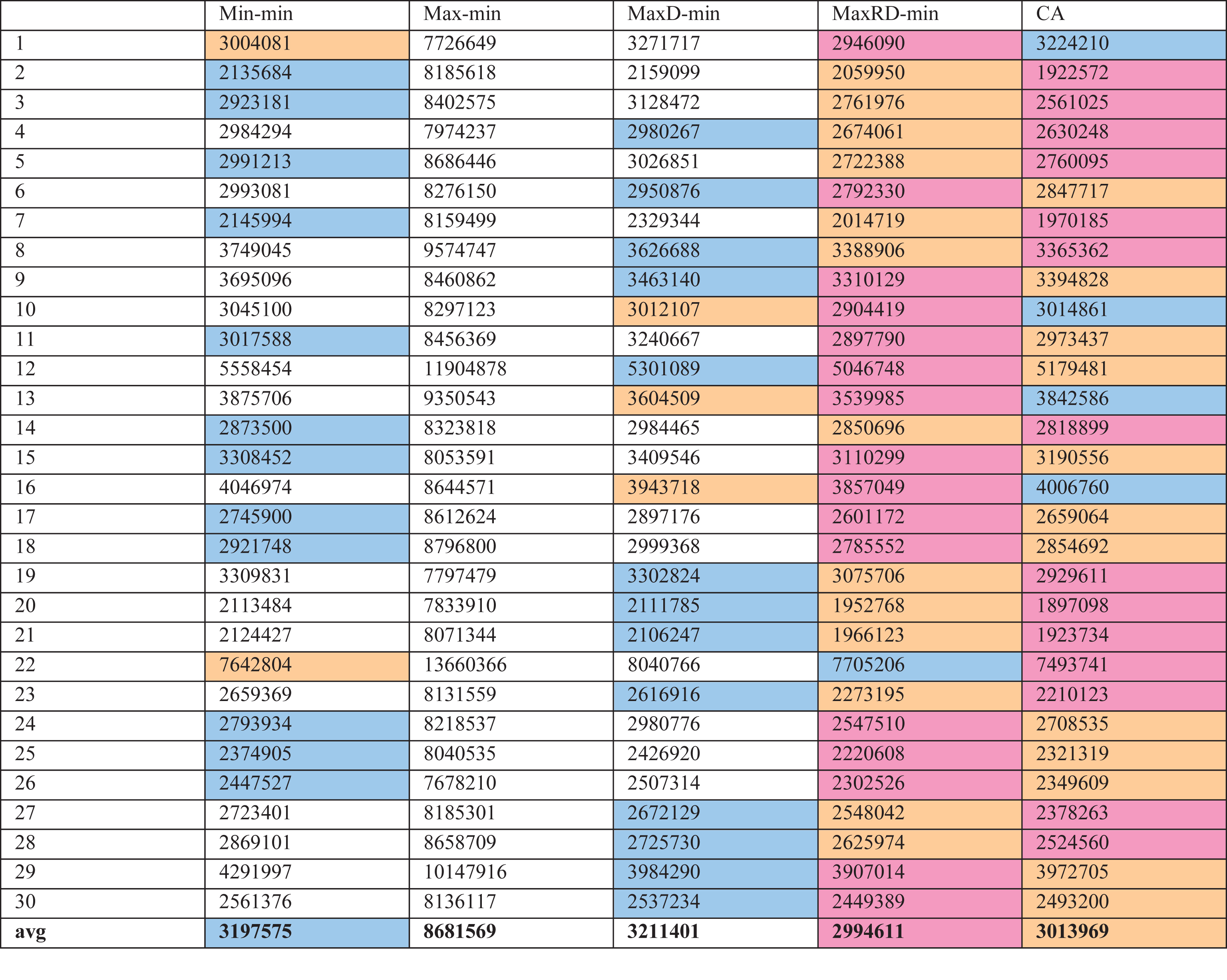
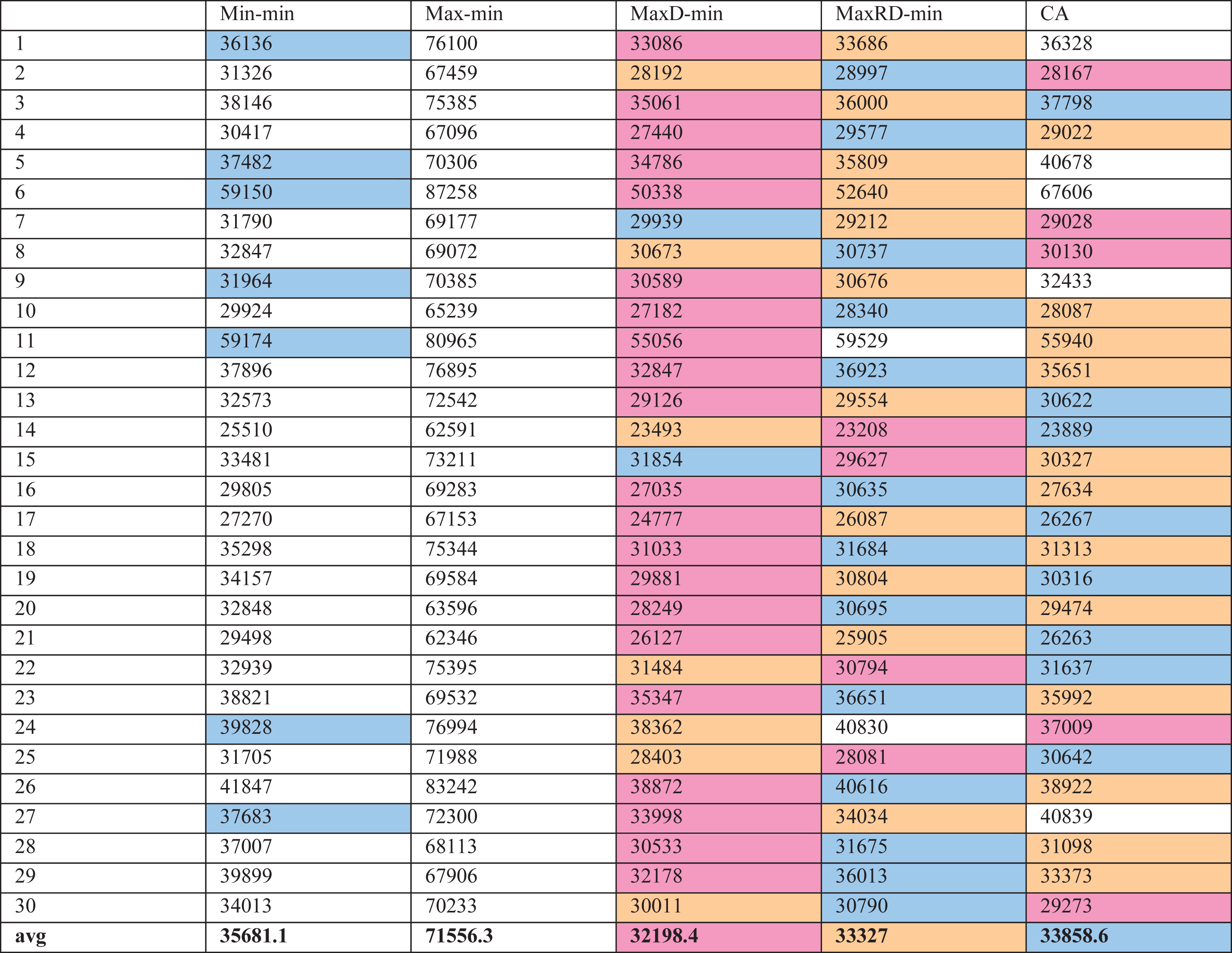
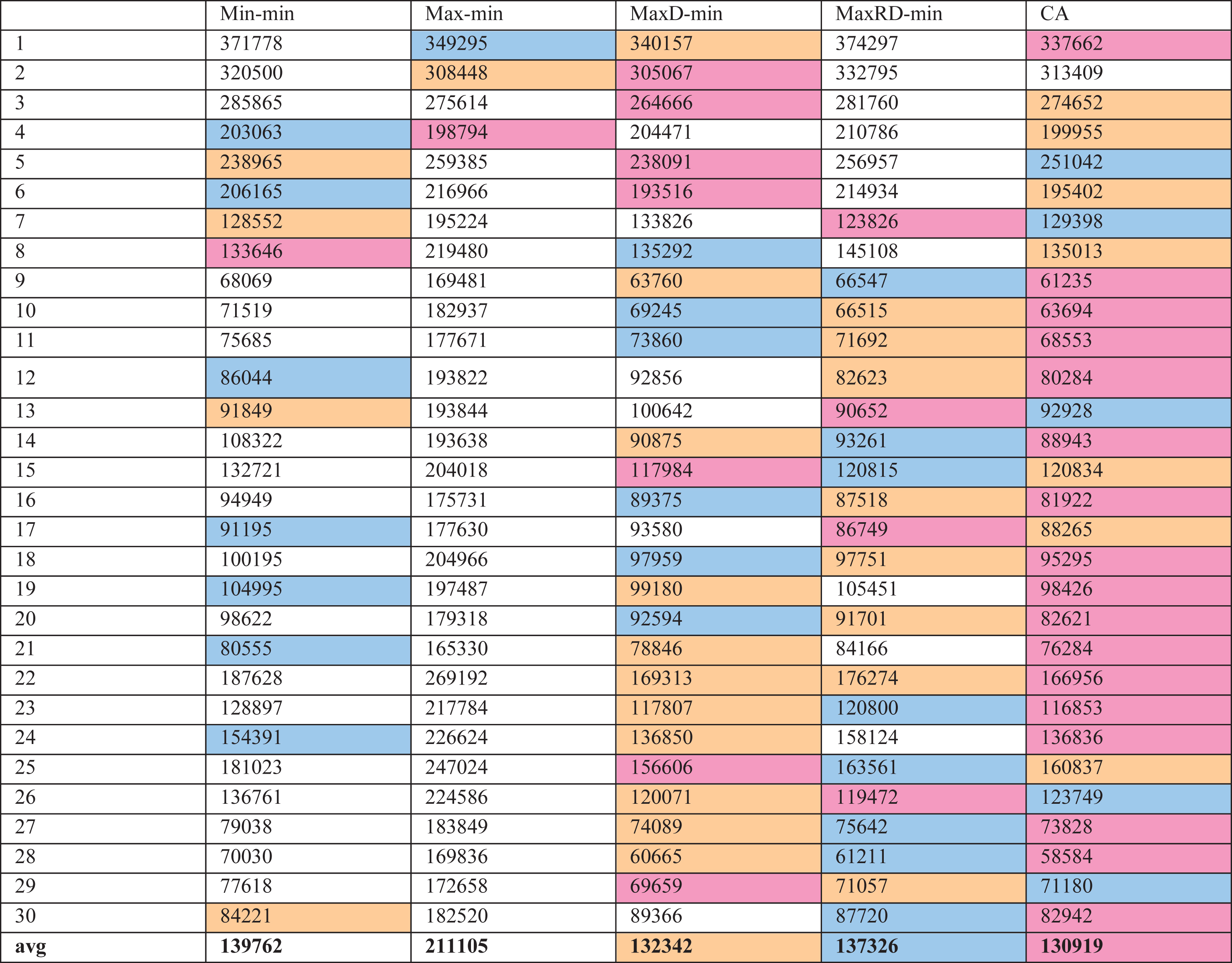
In doing so, 12 types of scences are set up in the experiment with 30 experiments in each setting. Algorithms including Min-min, Max-min and three algorithms given in this paper are adopted. The following is the results of 30 experiments in part of the settings, among which the best of makespan are painted in red, with the yellow as the second and the blue as the third (Table 3–5).

OPEN IN VIEWER

Table 4

Results of setting (256, 16, HTLM)

OPEN IN VIEWER

Table 5

Results of setting (128,8,LTHM)

The average bar values in the 12 types of scences are partly given in Figs. 1–4. From the left to the right are algorithm Min-min, algorithm Max-min, algorithm MaxD-min, algorithm MaxRD-min and algorithm CA. In each graph, the mark with the best makespan is painted in red, with the yellow as the second and the blue as the third.

OPEN IN VIEWER

Fig.1

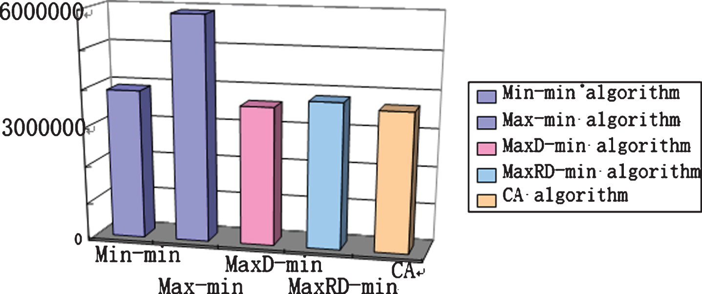
The Sence of (128, 8, HTHM).

OPEN IN VIEWER

Fig.2

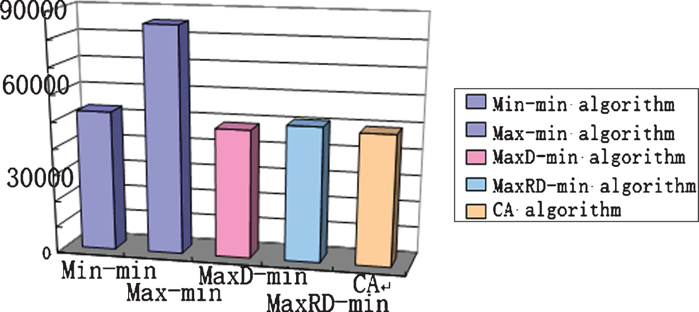
The Sence of (128, 8, HTLM).

OPEN IN VIEWER

Fig.3

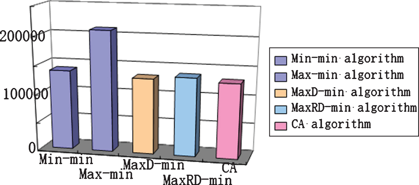
The Sence of (128, 8, LTHM).

OPEN IN VIEWER

Fig.4

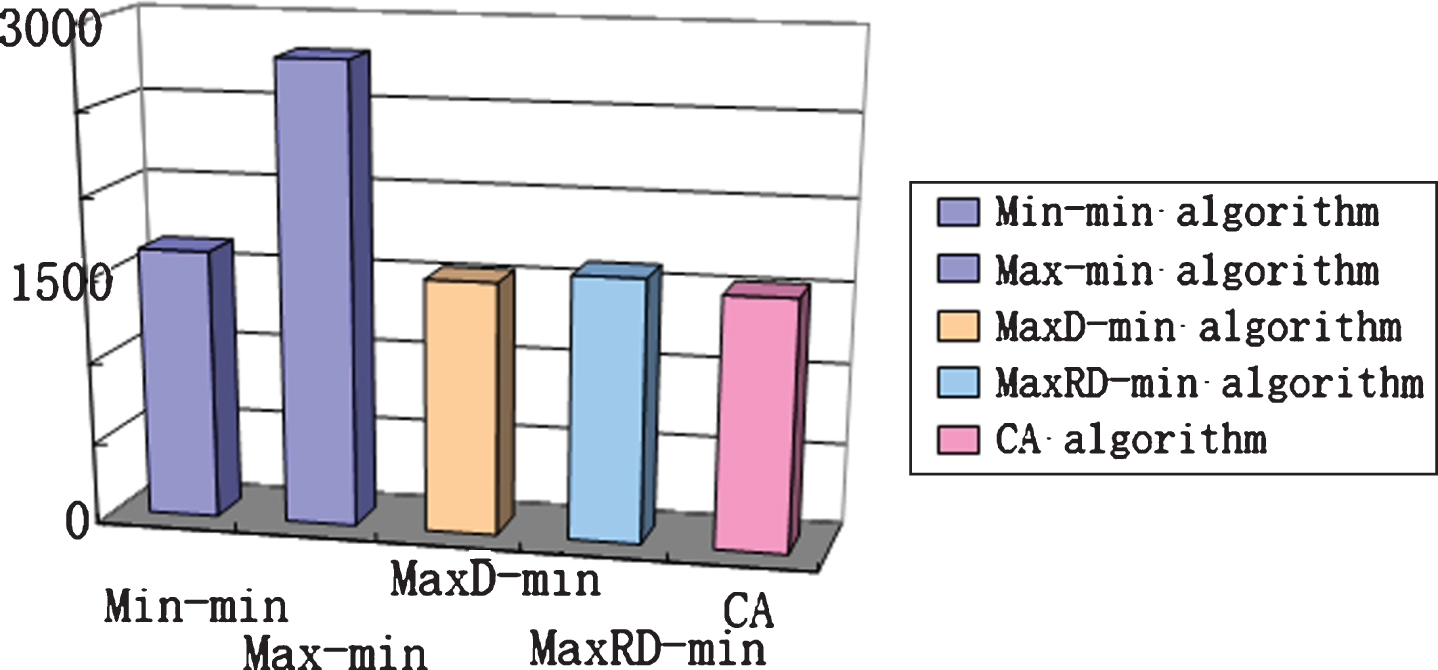
The Sence of (128, 8, LTLM).

In the 12 scences set up, the average makespan in the algorithm Min-min is much lower than the algorithm Max-min and in some cases, the average makespan in algorithm Max-min is several times higher than that in algorithm Min-min. Taking a single experiment into account, the algorithm Max-min in 300 experiments is superious to the algorithm Min-min but the time is less than 10. The way put forward in the paper is only compared with the algorithm Min-min. Table 6 gives the percentage increased for the 3 algorithms given in the paper than the makespan in the algorithm Min-min.

The followings are the results of three algorithms according to the experiments:

makespan in the algorithm MaxRD-min is 5 percent lower, on average, than that in the algorithm Min-min in all scenes. It is dramatically superior when the number of tasks is 128 or 256. It is not more complicated than the algorithm Min-min and it is of the same level of time complicated degree as the algorithm Min-min. Also, it can substitute for the algorithm Min-min in the batch tasks with small numbers.