Location estimation based routing for mobile adhoc network

Abstract

Mobile Ad hoc networks (MANET) are multi hop networks, which are self organized, self configured and their topologies are changed dynamically. The destination node may be out of range of source node and routes are changing with time due to mobility of nodes. So a routing procedure is required to establish a path between them to send packets. Based on mobility pattern of MANET nodes, we have proposed four reactive routing models of MANET, which utilize position information of GPS, enabled nodes to restrict the search of a new stable path in a smaller cone-shape request zone. Among the proposed models, first three are being recommended for open field networks whereas last one is for urban area networks. We have compared our models with LAR, LARDAR and TN-CMAD and have shown the proposed models performed better in terms of overhead packets and energy consumption but a little increase of path-finding error.

Keywords

MANET request zone expected zone routing link lifetime

1 Introduction

Ad hoc networks are multi-hop and infrastructure-less wireless networks where every node acts as either a host or a router, and it forwards packets to other nodes in the network. Due to their prospective uses in various situations like battlefield and emergency disaster relief, ad hoc networks have got widespread amount of interest. Ad-hoc networks are wireless networks where nodes use multi-hop links for communicating with other nodes. There is no fixed infrastructure or base station for communication. Routing in adhoc-networks has been a difficult task as network topology changes frequently due to mobility of nodes with high degree.

In past, works have been done on location prediction based MANET routing but in those works authors have not extensively studied mobility pattern and movement constraints of mobile nodes. In this paper we have considered those constraints and proposed four models of routing, based on their mobility which reduces overheads of route discovery by using position information of mobile nodes. Among the four proposed models, first three are related with mobility of nodes in an open field, and the last one is based on mobility in an urban area Mobile Adhoc Network. We have assumed nodes are GPS enabled and use GPS to get their position information. It is shown how the prediction of future position information can be used to limit the search of route discovery, which reduces overhead of route request packet in the network. If a node doesn’t find any path during route discovery, it can be termed as path-finding error. We have also shown the changes of path-finding errors of different routing models with the variation of density and transmission range of the nodes. During route discovery we have also considered more stable paths, which are not being used in any location based MANET routing in past.

2 Related work

Routing protocol design is a crucial problem in MANET. Various routing protocols have been proposed for ad-hoc scenario [5 , 19]. Johnson and Maltz [11] mentioned those routing protocols which are conventional and are not suitable for ad hoc networks. Because a large amount of bandwidth is wasted due to routing overhead, particularly the protocols where routing tables are updated periodically. They proposed a routing protocol using Dynamic Source Routing (DSR), which is an On-demand protocol, i.e., in the protocol routes are established when data transmission is demanded by a source host.

A number of protocols [10] optimizations are also being proposed which reduce overhead of route discovery. Perkins and Royer [19] proposed the AODV (Ad hoc On Demand Distance vector routing) protocol which is also an on demand routing protocol. In Zone Routing Protocol (ZRP), Hass and Pearlman [7] have combined proactive and reactive approaches, which initiate route discovery phase on-demand, but confine the scope of proactive procedure only to local neighborhood of source. Also, ZRP limits the topology update propagation to neighborhood of change.

Several locations based routing protocols [4 , 15] exploit location and node mobility information for routing process. Authors [21] have also proposed location based routing by using smart antenna instead of GPS receiver, whereas in [25] authors have proposed clustering technique in location based routing to handle larger mobile adhoc networks. LAR and DREAM [2, 13] are other two different location based routing protocols where in LAR, reactive routing protocol is used and its main aim is to discover route efficiently as well as reduce flooding of routing overhead packets. Using LAR, a node locates the zone of the destination node and it also includes location information in sent packets. In compare to LAR, DREAM is based on a proactive routing protocol and every node maintains location information of all nodes in the network. In DREAM, nodes update location information with certain frequency which is determined by relative distance between nodes and their mobility behavior.

Routing protocol [16] for MANET called “Location Prediction Based Routing” (LPBR) reduces number of route discoveries as well as hop count of the paths for a source-destination pair. LPBR collects information related to location and mobility of nodes in the network and saves the information at destination node while searching for a route. This information is used when minimum-hop route discovery using flooding fails. Then destination node tries to predict present location of each node. Due to mobility in MANET [18], topology of nodes changing frequently, where routing is a denoting challenge. This paper presents routing algorithm by predicting mobility of nodes and reduces overhead by eliminating sending of control packets which are required for route re-establishment. In this paper Hidden Markov Model (HMM) is used for predicting mobility of nodes. Authors also proposed proper allocation of resources and upgraded quality of service (QOS) by using mobility pattern.

In [1], authors have proposed another future position prediction based routing PLAR for MANET. In this paper, future position is predicted by using speed and direction of movement of nodes. Authors also used the concept of “information lifetime time” which is used to identify freshness of information about location. Authors have claimed that this idea gives more accurate information about nodes. Kai-Ten Feng and Tse-En Lu have proposed another routing protocol [6] (velocity aided routing (VAR)) for MANET. In the paper, proposed protocol determines a scheme of packet forwarding which is based on relative velocity between destination nodes and forwarding node. Routing performance is further enhanced by combining VLR and LAR routing protocol, which is called VLAR. Authors have worked with Gauss-Markov mobility model and constant speed mobility model in their proposed algorithms.

Future position of node also depends upon the mobility pattern of the mobile nodes. Random waypoint mobility model [29, 30] is one of the most studied and implemented models in MANET. Nodes move towards a direction for some time duration and then change its direction randomly with different velocity. Nodes pause for some time interval between moves.

In the paper [26], authors have proposed a Position based Opportunistic Routing protocol (POR), where forwarding nodes cache the data packets that have been received using MAC interception. Suboptimal candidates forward the data packets, if it is not done by the best forwarder. This process continues until one of the candidates receives and forwards the packet and thereafter the data transmission will be interrupted. The paper exploits potential multi-paths dynamically for each packet, which leads to POR’s excellent robustness. To overcome the communication hole, a Virtual Destination based Void Handling (VDVH) scheme is proposed which works along with POR.

Authors in the paper [27] have raised the drawback of POR, where severe drain of energy is happened at each node. Thus they proposed POR in combination with Quorum-based asynchronous power-saving (QAPS) protocol. This idea helps MANET to save more energy and can accommodate more hosts. Authors [28] have proposed Efficient Position-Based Opportunistic Routing (EPOR) protocol, which is stateless and highly dynamic in nature. The algorithm uses the property of overhearing, which helps identifying the network topology and reducing the latency of local route discovery along with the relay of duplicate packets. Authors have stated that Virtual Destination-based Void Handling (VDVH) with the combination of EPOR protocol in a communication hole, can give better performance even under high mobility.

Authors in the papers [17, 24] also used location information and proposed energy efficient routing in MANET network. Similarly authors in paper [22], have considered location based routing where minimum energy metric as well as multipath are considered and have compared the routing algorithm with LAR with varying number of nodes, pause time and speed. Another location based link state routing protocol LAGSR [12] is proposed, which reduces inaccuracy of routing due to topology change in high motion. Authors have assigned link weight, based on speed and relative position of node pair which reduces overhead of the routing protocol. This protocol is suitable for high speed MANET networks. The paper LAR²P [3] also considered location information of nodes and proposed a reactive flood-free routing protocol which has smaller path setup time as well as reduced control packets.

Authors in paper [23], have proposed routing LARDAR for MANET which is modified version of LAR. In LAR request zone is considered as rectangle whereas in LARDAR, request zone is considered as triangle for reducing broadcast overheads of route discovery. Authors of LARDAR also implemented dynamic adaptation request zone technique to find new request zone at intermediate nodes based on information they have. In paper [20] authors have proposed an routing algorithm which are also based on location of nodes and used two different techniques while forwarding data packets to their two hop neighbors towards destinations. But disadvantage of the algorithm is that every nodes periodically broadcast location information of their two hop neighbors to immediate neighbors, which actually have a large overhead for sending data packet. It has a fixed amount of overhead cost and thus this algorithm is only suitable where nodes always have large number of data packets for sending.

We have proposed four routing models which are based on mobility pattern of nodes. In first three models, open field networks are considered and in the final one, nodes are deployed in an urban area network. All these routing models are based on location of nodes and mobility pattern of nodes. Request zone is considered as cone shaped and has smaller area than above mentioned algorithms like LAR, LARDAR. These models help a node to find a destination node within a shorter zone, which reduces route discovery overhead in the network. We have addressed shortcomings of the above algorithms and propose modifications for improvement which are actually implemented in our proposed algorithms. We have also compared our first three models with LAR, LARDAR and TN-CMAD [20] in terms of number of route discovery overheads and path-finding error. Paths which are discovered by using proposed routing algorithms are more stable and reduce the requirement of frequent route discovery. Final model of algorithm is different from its predecessors and it is compared with LAR model, while both are used in same urban area network.

Motivation and our contribution are discussed in Section 3. In Section 4, we have discussed our four models for routing in Mobile Adhoc Network, where first three models are proposed for open field network (subsections 4.3.1, 4.3.2, 4.3.3) and last one is proposed for urban area network (subsection 4.4). Simulation and results are being discussed in Section 5 and finally in Section 6 conclusions have been drawn.

3 Motivation and contribution

In the routing algorithms LAR and LARDAR, authors have not considered mobility pattern of nodes and have calculated expected zone based on maximum speed of the nodes. But in real situation, actual expected zone is smaller in size because when a node moves, it changes direction several times and also gives pauses between moves. We have proposed three models of location based routing for open area network as well as one model for urban area network. In our work, we have considered all parameters like mobility pattern, speed and pause time, which help proposed algorithms to find out expected zone of MANET nodes. Request zone for LAR is considered as rectangle whereas in LARDAR, it is triangle in shape as shown in Fig. 1. Area of request zone of LARDAR is smaller than LAR, which helps to reduce route request overhead packets. In our work, we have reduced overheads further by decreasing expected zone as well as using cone shape request zone. In LARDAR, if nodes don’t find any neighbors in the request zone, it’s size is incremented gradually which eventually creates more delay in the system, We have also proposed a better technique to solve the hole problem, if arises in request zone. And finally, while route discovery, nodes choose the most stable path from source to destination so that frequent route discovery is not needed.

Fig. 1.

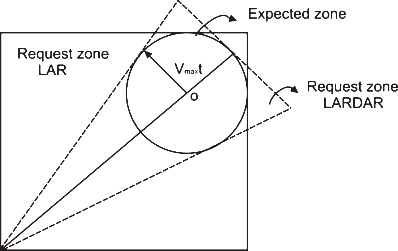
Expected zone and Request zone for LAR and LARDAR.

4 Proposed models for routing

We have proposed four models of routing which are based on mobility pattern of nodes. Where first three are considered for open area networks and final one is for urban area network. The basics of our proposed algorithms are same as the procedure of DSR and AODV with some levels of optimization are introduced in flooding of route request (RREQ) packets. Like DSR and AODV, when a node wants to send a packet to another node, it checks its routing table for a path to destination. If it does not find any path, it goes for route discovery using flooding method. It generates a route request (RREQ) packet and broadcast it. On the other hand, when route requests received by destination node, it constructs a route reply(RREP) packet which is based on route request packet. This unicast packet reaches to sender along the reverse path followed by the request. It is possible that destination node may not receive route request packet due to some communication error or due to some other errors like path-finding error. In that case source node resends the request. Path-finding error is one, where no path is available to reach to the destination. Our routing models are different from basic flooding algorithm, where in the proposed models path to destination is searched in a smaller region. Using position information, we attempt to narrow the zone, where route searching packets RREQ are forwarded. As a result, it reduces the number of routing overhead packets in the network. Before going to our proposed models, let us define two zones of the network which are as follows.

4.1 Expected zone

Consider a node S which wants to find a route from itself to another node D. It is assumed that S knows location of D at t₀ which is P and present time is t₁. Then expected zone of node D with respect to node S at time t₁ is the area where node D can be found at t₁. Node S can calculate expected zone by using both information, the location when D was at P at t₀ and the velocity of D. Suppose node D is moving with an average speed v, so it can move a distance in time duration t₁-t₀ is v (t₁-t₀). Thus expected zone of node D is the region of radius R = v (t₁-t₀) centered at P. If speed is more than average speed v then the node may go outside of the region. In case S does not know initial location of node D then whole region is considered as expected zone [13].

4.2 Request zone

This zone is used to send route request at time of route discovery. If a node belongs to request zone [13] it forwards route request, otherwise it drops it. For increasing the probability of successful reach of route request packets to node D, request zone should include the expected zone. In addition to it, request zone may also take other regions, which surround the request zone. Sometime it is not useful when request zone is small. Though it reduces flooding but it may not give guarantee that the route request reaches proper destination. On the other hand increasing request zone increases probability of reaching of route request to destination but also increases flooding of route request packets. Figure 2 shows both expected zone and request zone.

Fig. 2.

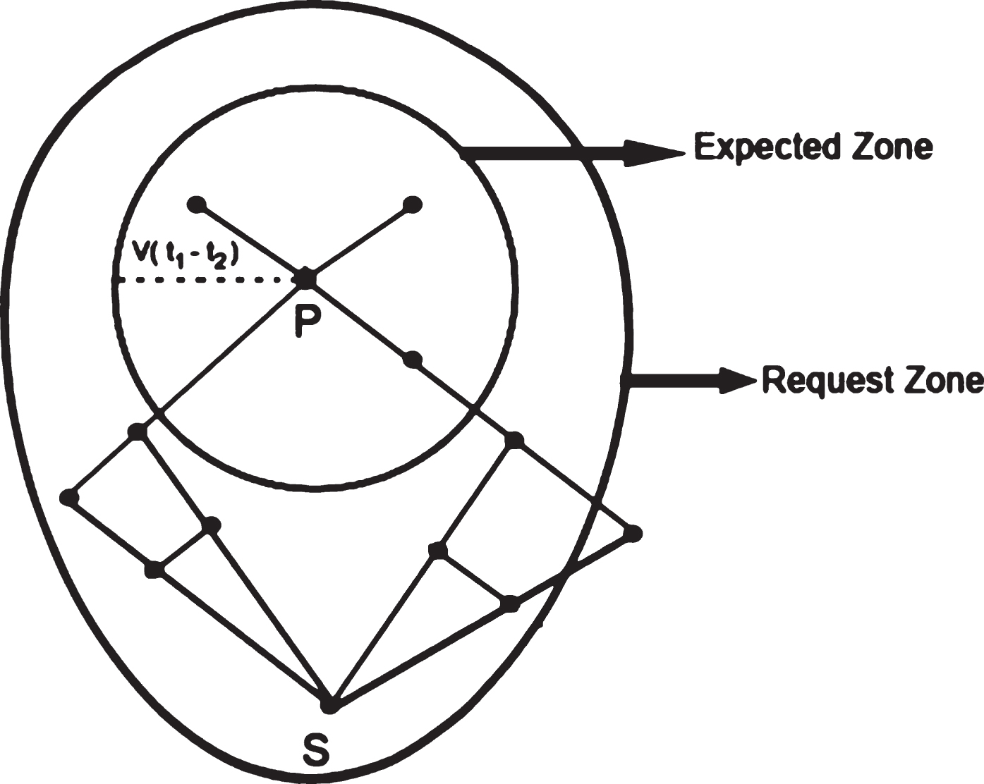
Expected zone and request zone [13].

4.3 Models for open area network

We have assumed that nodes are GPS enabled and able to get information by using GPS receiver. Suppose a node S knows location of another node T which is at P(x_p,y_p) at time t₀. At time t₁, S wants to send a packet to node T and the path between S and T has been expired. So S has to re-establish a new route to T. It is assumed that the node T is moving with an average speed v and that is known to node S. So the expected zone of node T is a circle of radius v(t₁-t₀) centered at point P(x_p,y_p). We have proposed a request zone which is a cone with vertex at S and it also includes the expected zone (shown in Fig. 4). Node S broadcasts RREQ packets in cone shape request zone, which reduces overhead of route discovery. In all three proposed routing models, we have used cone shape request zone. Mobility restriction is imposed gradually from Model-1 to Model-3. Main objective of these models are to reduce flooding of Route Request(RREQ) overheads. When expected zone covers node S then the request zone is a square, as shown in Fig. 3.

Fig. 3.

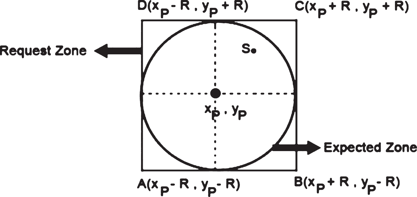
When S is inside the expected zone [13].

In the proposed routing models for open field MANET, random waypoint mobility is considered for first two models and in the third one, we have imposed some restriction on mobility which is useful for some real life applications. In random waypoint model, each node can move in any direction but it is fixed for some time interval δ and then there is a pause time t_p before next move. Instead of flooding RREQ packets in whole observed area, restricted broadcasting is used. Because when source and destination is far away then it is useless to search the destination thoroughly in a larger area near source, rather the area closer to destination should be large enough to get destination node available. The purpose of sending route-request packet is to search destination node in a specified area. In these models, node broadcasts RREQ packets in a smaller area when destination is far from source, but as destination gets closer, searching area is gradually increased.

4.3.1 Model-1

We have considered Random Waypoint mobility pattern for this routing model. Let maximum velocity of adhoc nodes is v_max. Thus at time t₁, node P must be anywhere in the area of a circle with center at(x₀,y₀) and radius is v_max(t₁-t₀), which is also the expected zone of node P. In this model we have considered a cone shape request zone, as shown in Fig. 4. Angle θ depends upon distance from source to destination, maximum velocity and elapsed time after t₀. There is an advantage of using a cone type request zone. When distance between source and destination is comparatively higher than the radius of expected zone, then angle θ has a lower value. It means search area (broadcast area of RREQ packets) is smaller near source and it increases as RREQ packets go closer to destination. But when distance between source and destination is comparable with radius of the expected zone then angle θ has a greater value. It means RREQ packets are broadcasted in a larger area. From the Fig. 4 angle θ can be calculated as . 3

Fig. 4.

Expected zone and Request zone for Model-1.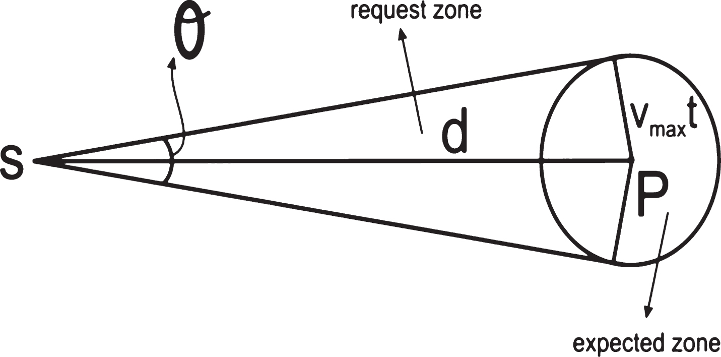

θ = 2 \arcsin (\frac{v_{\max} t}{d}) (0)

(0) when distance between source and destination is d and t = t₁-t₀. If we consider pause time(t_p) between moves, expected zone is further reduced. We are assuming that every average t_c time interval, nodes change the direction. At time t₀, when a source node notes last position of destination node then the later one is either in move or static for a maximum of t_p time unit. That means the destination node initially waits for an average of t_p/2 time from t₀ and then starts moving. Thus time difference between time(t₁), when source initiates path re-establishment with destination, and the time when destination starts moving after t₀, is Δt where

Δ t = t_{1} - t_{0} - \frac{t_{p}}{2}

(1)

So the number of pauses between this time interval is N_p, where $N_{p} = \frac{Δ t}{t_{c}}$ (2)

Destination node also takes a final pause of average time duration t_p/2 before t₁. So the node’s total pause time is $(N_{p} - \frac{1}{2}) t_{p}$ (3) and θ can be modified as $θ = 2 \arcsin (\frac{R}{d})$ (4) and $R = v_{max} (t_{1} - t_{0}) - (N_{p} - \frac{1}{2}) t_{p} v_{av}$ (5) where v_av is the average velocity of nodes. It is assumed that velocity of node is v_av, if it is in moving state during pause time. When source broadcasts RREQ packets, it attaches position (x₀, y₀), time (t₀) and θ of node P. Intermediate node whoever receives the packet broadcasts RREQ packet to its neighbors if it belongs in the cone shape region of angle θ. If receiving node has more recent position of destination, it calculates its own θ and uses in RREQ packets, otherwise θ remains same. If it does not belong in the region, then discard the RREQ packet. In all models we have considered that entire node’s clocks are time synchronised.

It may happen when θ is very small then there is not any path (path-finding error) in request zone due to unavailability of sufficient nodes in the region. In that case it is better to forward RREQ to a neighbor node, which is nearer to destination and has most stable link (longest lifetime). Thereafter neighbor node initiates broadcasting of RREQ packets to request zone for same destination. Here we have chosen a cut-off value of θ. If calculated θ is lesser than cut-off value, then source follows above mentioned procedure. Cut-off of θ is calculated in the following manner. From the Fig. 4, the area (A) of the request zone of the cone of angle θ is $A ≅ \frac{π (d + R)^{2}}{360} θ$ (6)

So the number of nodes are belonging to this area is $N^{'} = \frac{A}{L^{2}} N$ (7)

Where L is the side of square shape observing field where N numbers of nodes are deployed uniformly. If communication range is T_r, then minimum number(N_min) of nodes that is required to establish at-least one path between source and destination is (d + R)/T_r - 1. We have considered that the cone shape request zone must have at-least 2N_min nodes for broadcasting route request packets. So from above Equation (7) we can write $2 [\frac{(d + R)}{T_{r}} - 1] = \frac{A}{L^{2}} N$ (8)

Now from Equation (6), substituting value of A in Equation (7) and considering θ as θ_cut-off we can write $Θ_{cut - off} = \frac{2}{π} \times \frac{360}{T_{r}} \times \frac{L^{2}}{N} (d + R - T_{r})$ (9)

As we have used cone shaped request zone for all three models, so cut-off angle of θ is applicable for other two models also. We have also considered the path that is established by route discovery, has long life and a parameter LL (link lifetime) is used in RREQ packet. Initially the value is set as a very large value. Whenever a RREQ is broadcasted, every receiving node calculates lifetime of the link between itself to the sending node and set the parameter LL, where $LL = Min ({LL}_{old}, {LL}_{new})$ (10) where LL_old is the received LL value from the RREQ packet and LL_new is calculated lifetime. Lifetime of the link is calculated in the following way. Let two nodes A and B who are neighbors of each other. Position of the nodes are (x₁ - y₁) and (x₂ - y₂), velocity of the nodes are v₁ and v₂, and direction of movement are φ₁ and φ₂. Transmission range of the node is R and let after T time nodes are out of the range. So we can write

$\begin{matrix} [{(x_{1} + v_{1} T c o s ϕ_{1}) - (x_{2} + v_{2} T c o s ϕ_{2})}^{2} \\ + {(y_{1} + v_{1} T s i n ϕ_{1}) - (y_{2} + v_{2} T s i n ϕ_{2})}^{2}] \\ = R^{2} \end{matrix}$ (11)

So $T = \frac{- (mn + op) + \sqrt{(m^{2} + o^{2}) R^{2} - (mp - on)^{2}}}{(m^{2} + o^{2})}$ (12) where $m = v_{1} \cos ϕ_{1} - v_{2} \cos ϕ_{2}$ (13) $o = v_{1} \sin ϕ_{1} - v_{2} \sin ϕ_{2}$ (14) $n = x_{1} - x_{2}$ (15) $p = y_{1} - y_{2}$ (16)

When a node (other than originator) broadcasts RREQ packet, it uses the value of T as new value of LL(LL _new ), and modifies LL parameter of RREQ packet according to equation mentioned above. Destination node waits for some time interval δt (2× propagation time from source to destination) and receives all RREQ packets and chooses the path for sending route reply which has maximum value of LL. This method establishes a path of longest lifetime among paths available in the request zone.

4.3.2 Model-2

Though in the earlier model(Model-1), expected zone calculation is based on maximum velocity v_max of nodes, but it is unusual that nodes always move with that velocity and it is also rare that nodes moves with same direction for a long time. Thus, generally actual expected zone is smaller than the previous one. Even if the node always moves with maximum velocity, still expected zone is smaller in size due to its mobility pattern. From Fig. 5, it is seen that if node changes its direction with a large angle from its previous direction then it cannot go very far from its initial position, but if angle is very small then displacement is more than the former one. In both cases actual distance from initial position is smaller than v_maxt. So the expected zone have a radius R, where

Fig. 5.

Mobility pattern of Model-2.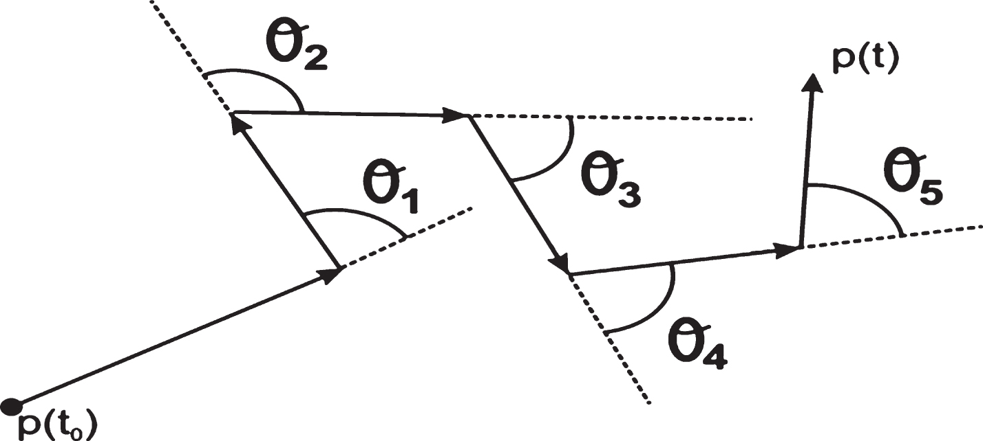

R = v_{\max} t - α v_{\max} t = v_{\max} t (1 - α)

(17) where α is factor which depends upon the mobility of node. We have given an expression of α.

α = \frac{1}{180} (\frac{\sum_{i = 1}^{n} θ_{i}}{n})

(18) where n is number of direction change and θ_i is change of direction in ith epoch.

When θ is more than 180° then it actually changes its direction by 360° - θ in opposite direction. So maximum direction angle change is bound to 180°. Thus $0 \leq α \leq 1$ (19)

Every time when nodes are changing their direction by large angle then the value of α is high. It creates a smaller expected zone. But if the direction change is smooth, α becomes low which creates a larger expected zone. Whenever a node changes its direction, it recalculates its α value, and nodes who have already established a path to that node should have information about α along with the position information of the nodes.

This model is same as the Model-1 except some modifications have been done while considering the expected zone. Source node who wants to establish a path to a node, calculates the expected zone by considering the value of α and find cone shape request zone by calculating θ by using the same method as Model-1. Again considering pause time t_p, expected zone can be reduced further. As the number of direction change is n, so it pauses for a total time nt_p.

So the radius (R) of the expected zone is modified to $R = v_{\max} t (1 - α) - {nv}_{av} t_{p}$ (20) where v_av is the average velocity. For onsidering stable links, we have used same methods like Model-1.

4.3.3 Model-3 (restricted random model)

Here we have imposed some restriction on mobility of adhoc nodes. In this model nodes cannot move in all direction. It has N_d numbers of equally spaced (θ) directions, where θ = 360/N_d. Generally robots carrying nodes have this type of movement. In Fig. 6 we have taken, N_d is equal to 8 and thus θ = 45°. We have also assumed that nodes changes its direction in every average time interval (t_a) and maximum velocity is v_max. In Fig. 7, movement of a node is shown, where it moves a distance b (where b = v_maxt_a) then changes direction of angle θ (45°) at A then moves a distance b again and changes its direction again by same angle at B and moves so on in same manner. When a node moves through a path shown in Fig. 7, the displacement is equal to the euclidean distance from starting point p (t₀) to p(t). Let T is the time duration between the time, when a node knows last position of destination and present time. Thus in this time duration a node P changes its direction n times. where

Fig. 6.

Model-3: 5(a) Number of change of direction is 360/θ 5(b) When θ = 45°.

Fig. 7.

Maximum distance covered by node p of Model-3 in time (t-t₀) is the dotted line from p(t₀) to p(t).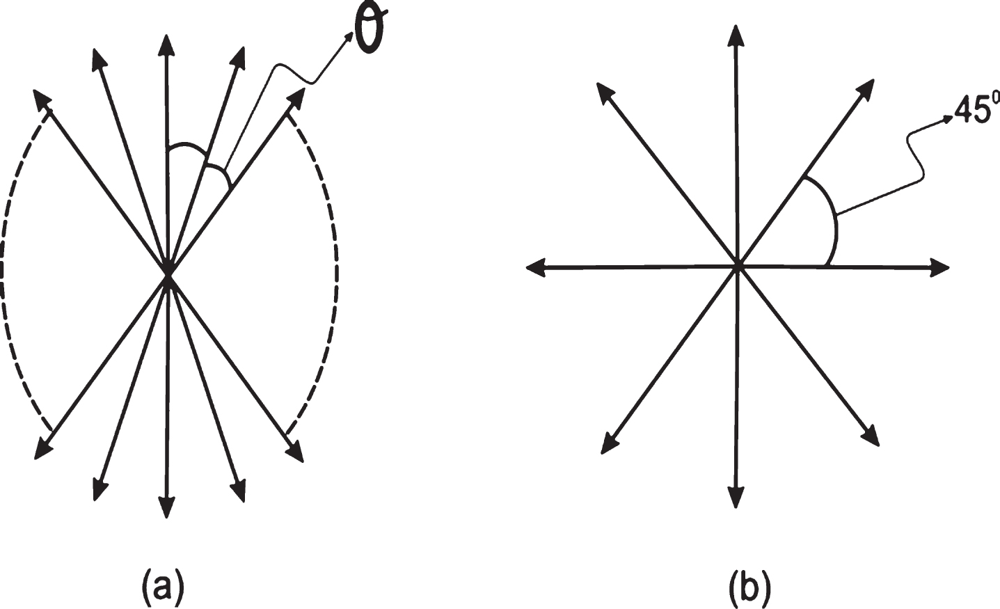

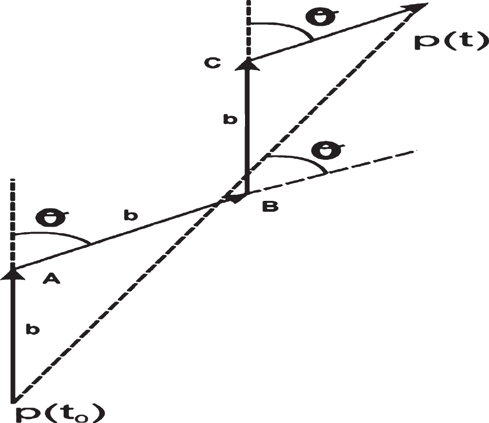
n = ⌈ \frac{T}{t_{a}} ⌉ - 1

(21) if n is not a integer multiple of t_a then in the last move it proceeds towards a particular direction for a time duration of t′, where t′ < t_a and t′ = (T - nt_a).

So within time T, a node can move a maximum euclidean distance D which is based on even and odd value of n. If n is even, maximum euclidean distance D is

$\begin{matrix} D & = & \sqrt{{(\frac{n}{2} v_{\max} t_{a} + {lv}_{\max} t^{'} + \frac{n}{2} v_{\max} t_{a} \cos θ)}^{2}} \\ \bar{+ {(\frac{n}{2} v_{\max} t_{a} \sin θ)}^{2}} \\ = & v_{\max} t_{a} \sqrt{{(\frac{n}{2} + l)}^{2} + \frac{n^{2}}{4} + n (\frac{n}{2} + l) \cos θ} \end{matrix}$ (22.1)

If n is odd

$\begin{matrix} D & = & \sqrt{v_{\max}^{2} t_{a}^{2} {(⌈ \frac{n}{2} ⌉ + ⌊ \frac{n}{2} \sin θ + lcos θ)}^{2}} \\ \bar{+ v_{\max}^{2} t_{a}^{2} {(⌊ \frac{n}{2} \sin θ + lsin θ)}^{2}} \\ = & v_{\max} t_{a} \sqrt{{(⌊ \frac{n}{2} ⌋ + l)}^{2} + {(⌈ \frac{n}{2} ⌋)}^{2}} \\ \bar{+ 2 (⌊ \frac{n}{2} ⌋ + l) (⌈ \frac{n}{2} ⌉) \cos θ} \end{matrix}$ (22.2) where $l = \frac{t^{'}}{t_{a}}$

Like earlier two models, considering the pause time t_p between moves, distance D can be reduced by an amount of nv_avt_p.

So the expected zone of the node is a circle of radius D with center at (x₀, y₀) which is assumed the last known location of the destination. Like earlier models, request zone is also a cone. Every node which receives RREQ packets and belongs to this request zone, broadcasts RREQ packets but the request zone is recalculated based on its own position and the destination node’s position. In this model we have used same logic (mentioned in earlier models) to establish a path which has a longer life.

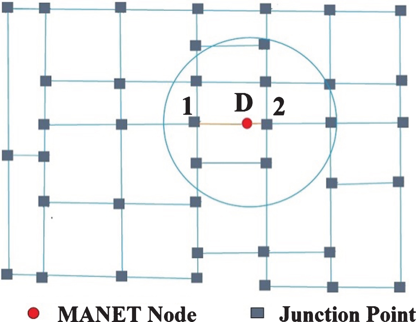
4.4 Model for urban area network (Model-4)

In this section we have proposed a model which is used to predict the future position of the nodes that are deployed in an urban area. In urban scenario, nodes cannot move freely in all directions, but can move through available roads (shown in Fig. 8) only. We have assumed that all the nodes have co-ordinate information of the junction points of all roads of deployment area. Thus, Fig. 8 can be represented as a road graph where junction points of the roads are the vertex of the graph and edges are roads between the junction points. We have also assumed that nodes are also equipped with GPS receiver for finding out their location information and the road graph is available to each node in the network.

Fig. 8.

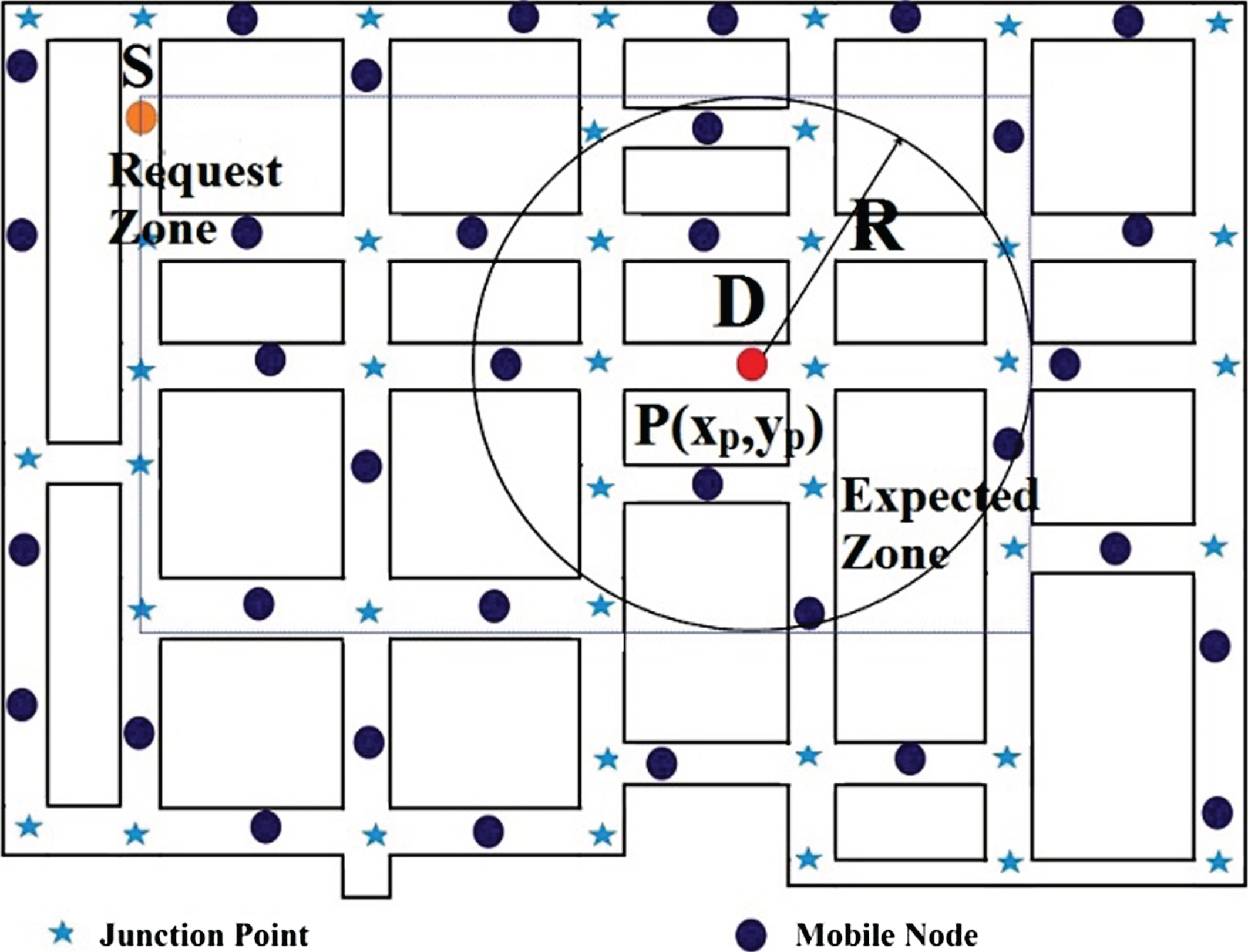
Urban Area MANET Network.

In Fig. 8, let node S which wants to communicate with node D at time instant t₁. It is assumed that S knows the position (x_p, y_p) of D at t₀, which is point P. As nodes have restricted movement in the deployment area, earlier proposed methods for finding expected zone and request zone are not suitable for this environment. Thus, we have proposed an algorithm (given next) to find the expected zone of destination node D at t₁ as well as the request zone for source node is S. As road graph is available to each node and source node S knows the position of node D at time t₀, thus the road graph can be modified into a new graph with the inclusion of node D as a new vertex at position (x_p, y_p) (shown in Fig. 9). Let node D is moving with a average velocity v. Expected zone of node D at time t₁ is a circle with center at P and radius R, which is possible distance traveled by node D. Thus it is the problem of finding longest path in the modified road graph which is actually a NP complete problem. We have proposed a heuristic to find out the longest path with the help of finding shortest time path, which is discussed below.

Algorithm: Expected Zone Algorithm for Urban Area Network

//Input: Road graph and positional information of source //and destination at time t₀.

//Output: Expected zone of destination at time t₁.

// P is the point of destination node D at time t₀.

1: d_i is distance of node v _i from point P.

2: R = v(t₁ - t₀) // R is the radius of expected zone

3: for (each vertex v _i ) do

4: if (di ≤ R) then

5: Add <d_i, I >in list L

6: end if

7: end for

8: Sort L in descending order of distance

9: for (each item j in list L) do

10: k = vertex in j^th entry of list L

11: compute shortest time(t_s) from D to vertex k

12: if (t_s ≤ (t₁- t₀)) then

13: t_r = (t₁ - t₀) - t_s

14: R = d_k + vt_r

15: break

16: end if

17: end for

Fig. 9.

Road graph of Urban area.

Let d_max is the maximum distance which is travelled by node D in time interval T (= t₁ - t₀), where d_max ≤ vT. Node S uses a list L to store the N vertices, who belong within the circle with center at P and radius is vT and arranges the list L in descending order of their euclidean distances from the center P. Considering node velocity v, cost of each link of road graph (Fig. 9) can also be represented in terms of time which is (d/v), where d is cost of the link in terms of distance. Node S finds the shortest time paths of all nodes in list L and selects the first vertex v_n(x_n, y_n) from beginning of the list with shortest path cost t_n, where t_n ≤ T. Thus, in time interval T, D can move from its position P is Rwhere $R = d (P, v_{n}) + v (T - t_{n})$ (23)

d(P,v_n) is the euclidean distance between P and vertex v_n. Thus, the expected zone is a circle centered at P with radius R and the request zone (shown as dotted rectangle in Fig. 8) is like LAR model, which includes the expected zone. Nodes are not available everywhere inside urban area due to their movement through available roads only. Thus, we have chosen the request zone as a rectangle instead of cone to reduce path-finding error in urban area network. Proposed algorithm to find the expected zone in urban area network is given next.

Here we have shown the proposed algorithm works correctly to find the expected zone of a destination node in an urban area. We have used following notations

v_i: Vertex i of road graph

L: Set of ordered list of vertices whose distances from point P are in descending order.

d(v_i): Euclidean distance from P to vertex v_i.

S(v_i): Shortest cost path form P to vertex v_i in terms of time.

From the proposed algorithm the list L can be written as $L = {v_{i} | vT \geq d (v_{i}) \geq d (v_{i + 1})}$ (24)

The farthest junction point in list L that can be reachable within time T is say v_n. Thus $S (v_{n}) \leq T$ (25) and $S (v_{i}) > T, \forall i < n$ (26)

Let us assume there is another vertex v_m available, where d (v_m) > d (v_n) and satisfies the following conditions $S (v_{m}) \leq T$ (27) and $vT \geq d (v_{m})$ (28)

But to satisfy these conditions, v_m ∈ L and m < n. But v_n is the first node in list L which satisfy the Equations. (25, 26). So there must not be any node v_m before v_n in the list. Thus it shows our assumption is wrong and proved v_n is the farthest junction point, where a node can reach from the point P within time interval T.

4.4.1 Complexity of algorithm

Let the number of junction point in the urban area is N_j. Initially the algorithm takes O(N_j) to find the junction points which belong inside the circle centered at D with radius is equal to vT. It also takes O (N_jln (N_j)) to sort the distance of the junction nodes of that circle. Finally, It takes $O (N_{j}^{2})$ to find out the shortest time path of all junction nodes of the circle. Thus, overall time complexity is $O (N_{j}^{2})$ where N_j is fewer than total number of MANET nodes. If each adhoc node calculates shortest time path(considering maximum speed of MANET nodes) from each junction node to other junction nodes beforehand then this cost can be used to find the shortest time path to all nodes inside the circle from the MANET node D as shown in Fig. 9. The preprocessing cost of calculating shortest path is done only once before start of the algorithm and it is fixed. Only the information that is required is the time cost from node D to its neighbor junction nodes. In the Fig. 9, the shortest paths from node D to all junction nodes are calculated by considering the time costs from D to node 1 and 2 along with the shortest cost paths from node 1 and 2 to other junction nodes. Thus, if the preprocessing fixed cost is not considered then the time complexity of finding the shortest cost path is O (n_bN_j), where n_b is average number of neighbor junction nodes of a MANET node. Considering n_b as constant, overall time complexity is O (N_jln (N_j)).

5 Simulation and results

Simulation is done using simulator software Omnet++ 4.3. We have considered two types of MANET networks where in first one, nodes are placed in an open field and in later one, nodes are placed in an urban area. In first part of simulation, we have considered the network of first type where number of nodes has been chosen to be 50, 100 and 150 for different simulation runs. The nodes in this adhoc network are confined to a 1000×1000 unit square region. We have considered the said mobility patterns for implementing the models. For these models, maximum velocity of nodes are chosen as 10, 15, 20, 25 and 30 units/sec and transmission range of each node chosen as 150, 200 and 250 units for different simulation run. We have considered wireless channel with a data rate of 1 Mbps. Data packet size has been chosen 1024 bytes and overhead packets (RREQ and RREP) size are chosen 32 bytes. We have considered IEEE 802.11 as MAC protocol and all simulations are continued for 100 seconds. Data packets, that are generated from nodes follow Poisson distribution with an average data packet rate is considered 5 packets/sec in most of simulation runs.

During simulation each node makes several moves and gives pause of 1 second between moves. After moving of 15 units, each node’s position is updated. Every time each node changes its direction in random manner after moving a distance of 100 units. θ for Model-3 is considered as 45°. While move, if a node hits the boundary of 1000×1000 region, node changes it’s direction and continues moving in same direction for remaining distance. In simulation we have chosen source and destination nodes randomly. In first part of simulation, we have studied the proposed models and have compared with LAR [13], LARDAR [23] and the routing algorithm TN-CMAD [20].

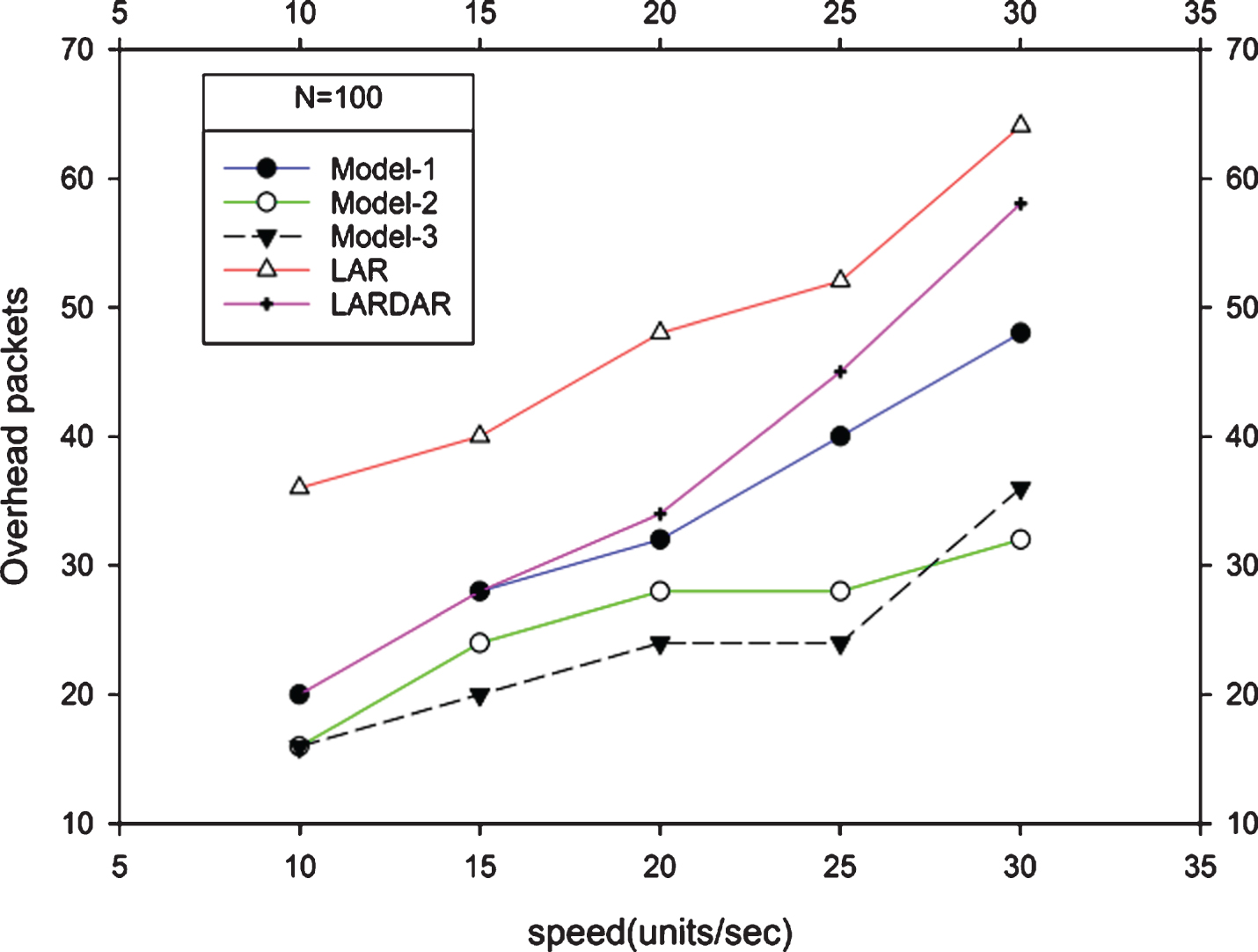
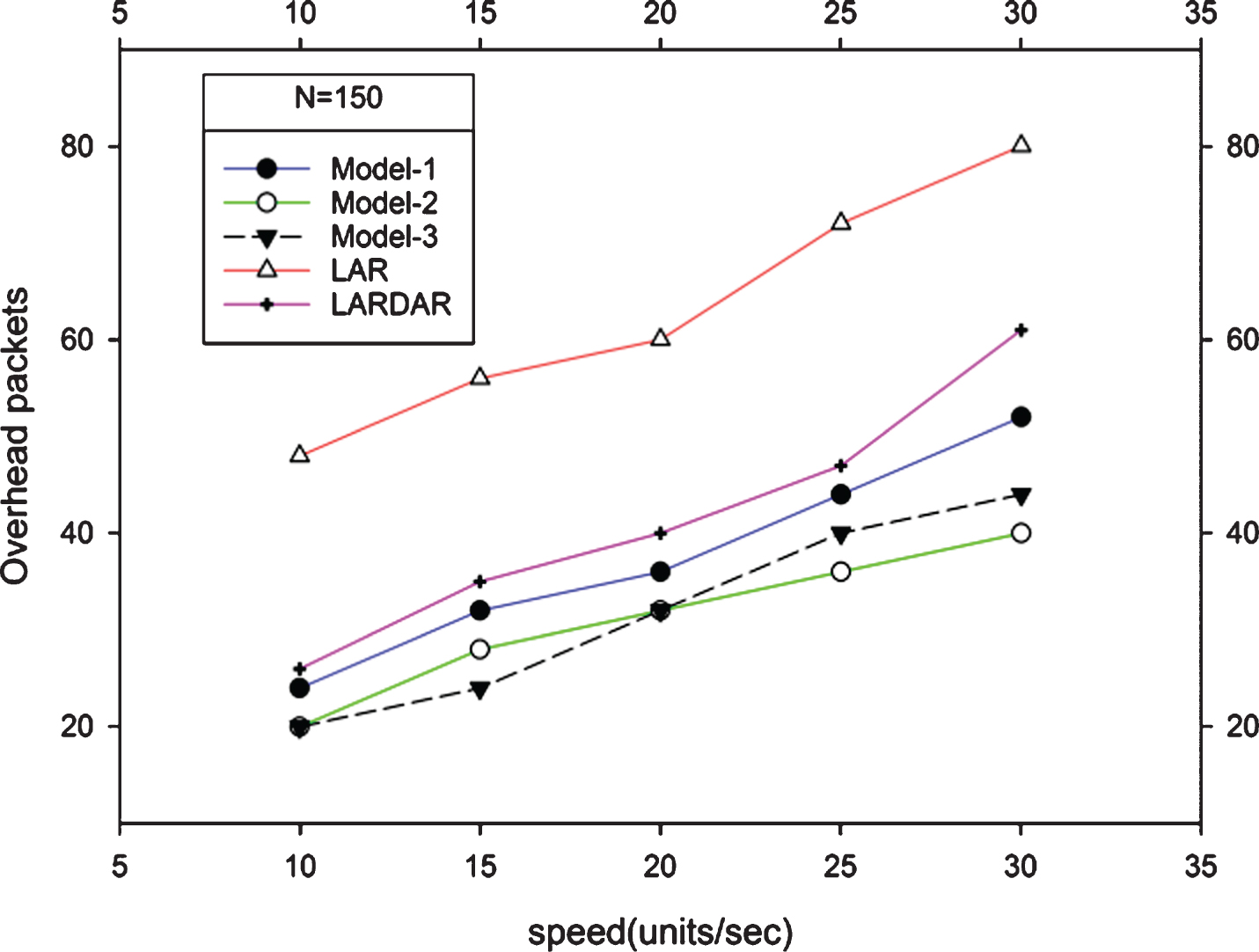
In first set of simulation, transmission range of node has been chosen as 150 units and speed of the nodes is varied in different simulation run. Each set of simulation has been done several times to take average of the result. In the simulations, we have calculated the number of RREQ packets that are broadcasted by the nodes for each route setup, where source and destination are chosen randomly. Figures 10–12 demonstrate the number of RREQ packets transmitted by the nodes for route setup with varying node speed. From the figures, it is found that our proposed models perform better than LAR and LARDAR methods. In almost all cases of different number of adhoc nodes, number of RREQ packets transmission is lower in the proposed models.

Fig. 10.

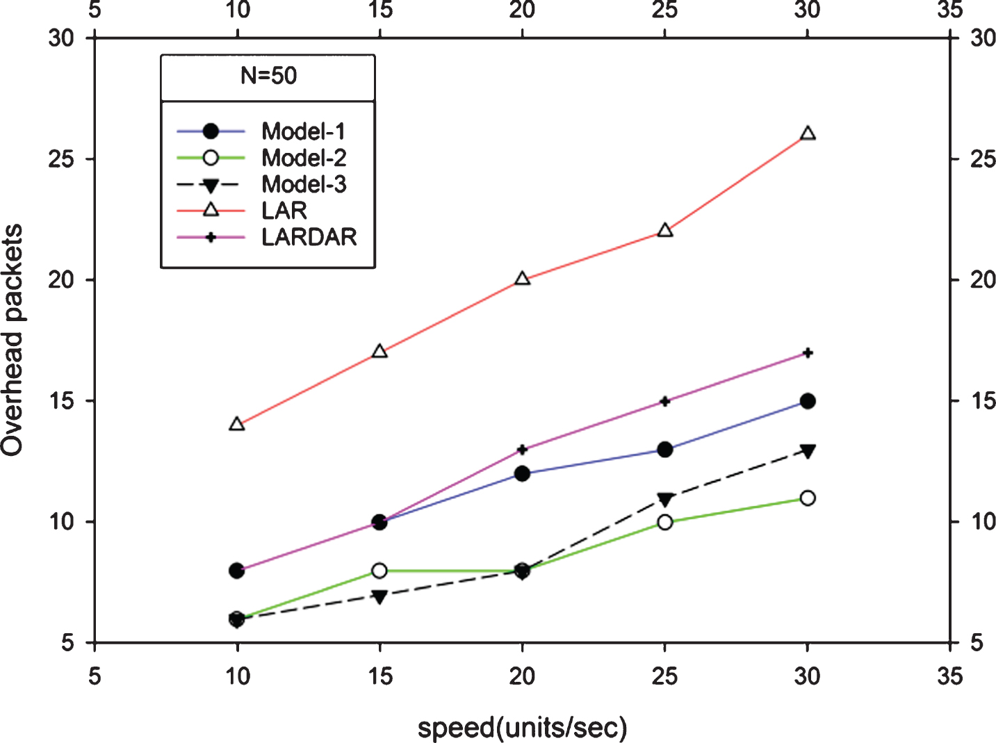
Number of nodes is 30.

Fig. 11.

Number of nodes is 40.

Fig. 12.

Number of nodes is 50.

On the other hand, request zone of Model-2 is smaller than Model-1. Thus, RREQ packets transmitted in Model-2 is lesser than Model-1 and similarly Model-3 also performs better than Model-1. As mobility pattern of Model-2 and Model-3 are different, so it is useless to compare them with each other. It is also observed that as speed of nodes increases, RREQ packet transmission also increases in all models. It happens due to more frequent breakup of links that occurs among the nodes, which needs more frequent path setup between them. Similarly, for a constant speed when number of nodes are increased, number of RREQ packets also increases because request zone contains more number of nodes.

When a node broadcasts a single RREQ packet, it is received by all of its 1st hop neighbors. So for single RREQ broadcast corresponds to more than one RREQ packet reception. Like transmission, nodes also use some energy for receiving data. So more energy is used in the network, when number of received RREQ packets are more. In next three Figs. 13–15, we have shown the energy consumption of nodes for establishing a new path. Nodes in the request zone spend energy for transmitting and receiving RREQ and RREP packets in the network. Thus total energy consumption for establishing a new path from a source to a destination is summation of all spent energies of all the nodes in the request zone.

Fig. 13.

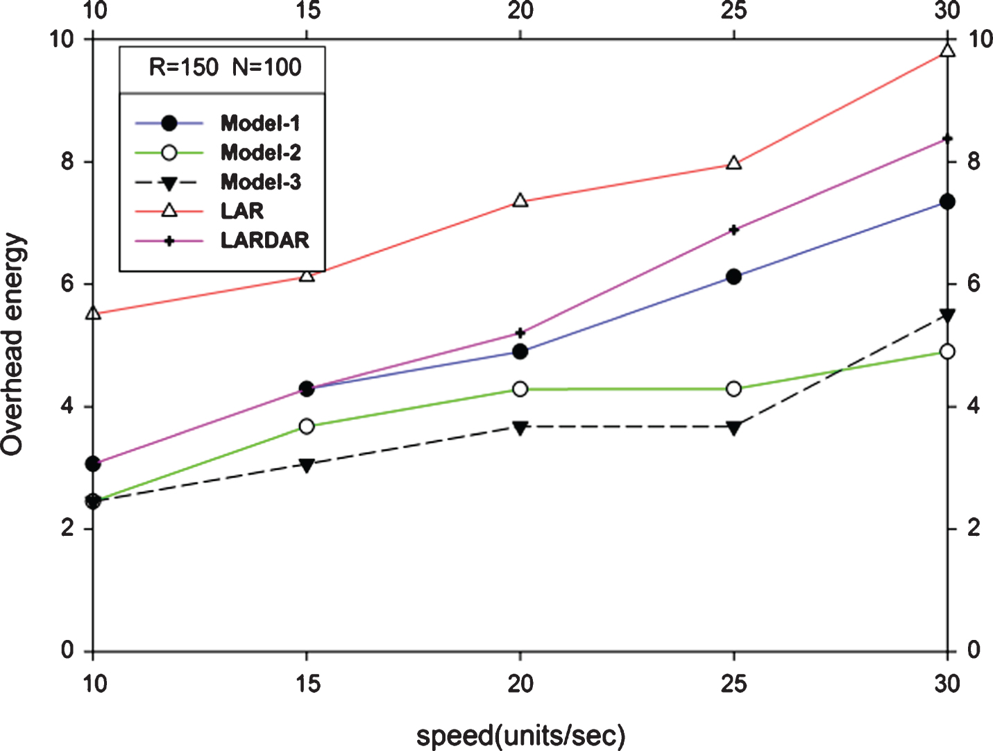
Transmission range is 150.

Fig. 14.

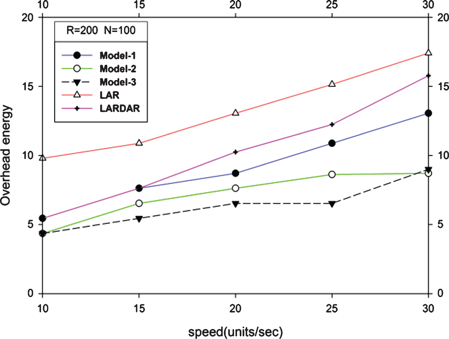
Transmission range is 200.

Fig. 15.

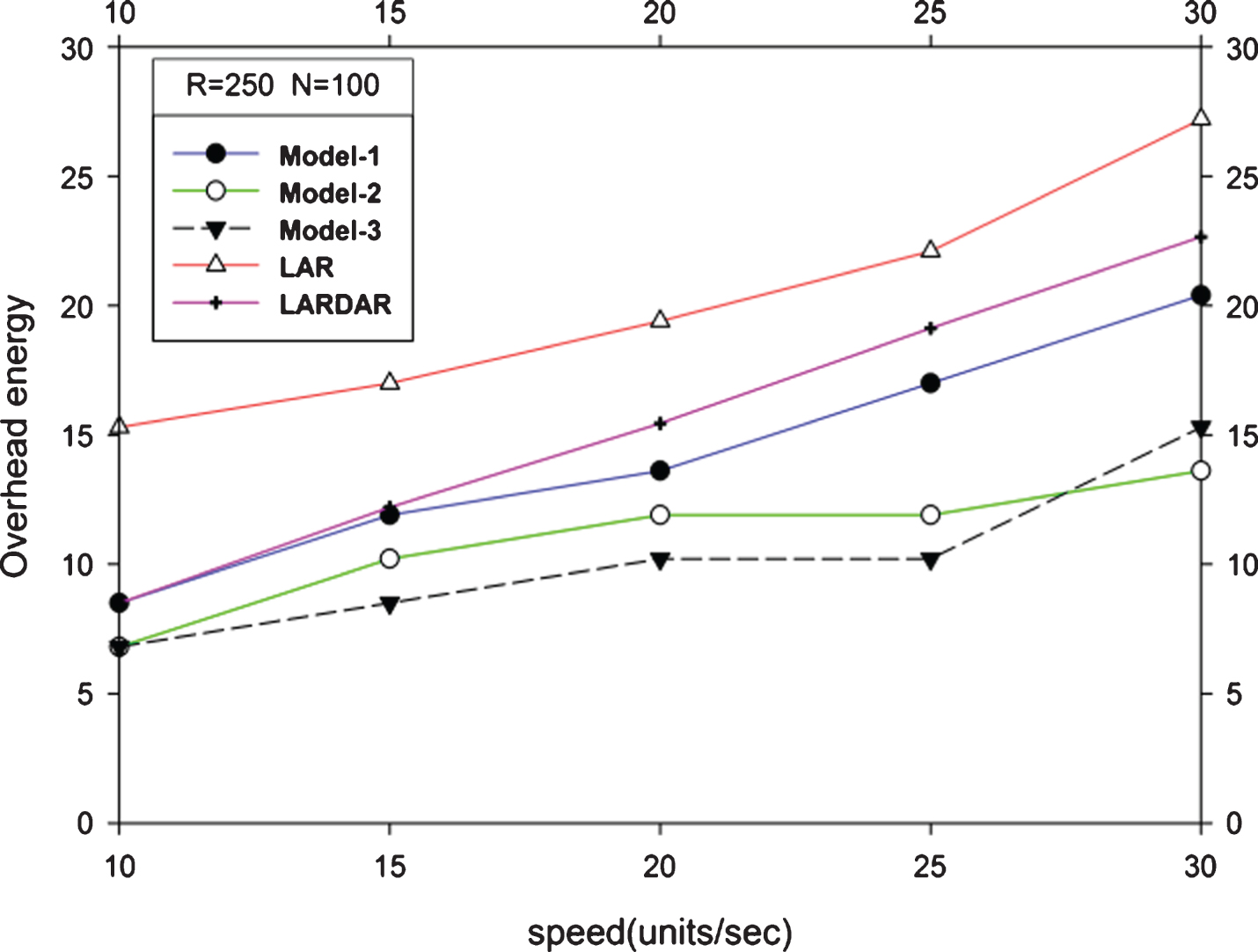
Transmission range is 250.

We have considered a first order radio model, where energy consumes by the radio is E_tx to transmit a k bits message over a distance of d. $E_{Tx} (k, d) = E_{elec} \times k + ɛ_{amp} \times k \times d^{2}, d > 1$ (29)

Therefore, the power consumption of data transmission between two nodes is proportional to the square of their distance. Similarly energy consumption while receiving of data $E_{Rx} (k) = E_{elec} \times k$ (30)

While k is the data volume to be transmitted (bit), d is the distance between two nodes, E_elec is the energy consumption to carry out data transmission in terms of nJ/bit, ɛ_amp is the energy consumption constant used to expand radio coverage in terms of nJ/(bitxm²).

Total consumed energy of each node is equal to ∑E_RX + ∑E_Tx, which is the sum of total consumed energy of data receiving and total consumed energy of data transmitting. E_elec is considered as 50 nJ/bit and ɛ _amp is consider 100 nJ/(bit . m²).

We have varied the transmission range of nodes from 150 units to 250 units and number of nodes is fixed to 100. From the graphs it is found that with the increase of transmission range, received overhead packets (RREQ) increases due to increase of number of neighbors. Thus, here also our proposed models perform better than LAR and LARDAR. Like earlier, Model-2 performs better than Model-1 due to smaller request zone.

We have also studied overhead energy consumption of TN-CMAD routing that is proposed in [20] and have compared it with our Model-1. First a mathematical analysis is given then simulation results are compared.

Let there are N number of nodes in the network and every τ time interval, nodes broadcast all its neighbors information to its one hop neighbors. It helps every nodes to know about the nodes within two hops. Considering the transmission range R of the nodes, average number of neighbors (n_av) of each node is $n_{av} = \frac{π {NR}^{2}}{L^{2}}$ (31)

L is the length of the square shaped deployment area. Broadcast packet size is increased with increase of neighbors because more bits are required to include all neighbor’s information. Increase of transmission range does increase the number of neighbors and thus the broadcast packet size. So the overhead energy consumption E_ov can be written as $E_{ov} \propto {Nn}_{av} R$ (32)

It is found from above equation that cost E_ov for each interval is constant for fixed R. Thus, if only few nodes send data packets in the interval or R is increased, then overhead cost per data packet is more. By doing simulation, we have shown it in Fig. 16 and also compared with our routing Model-1.

Fig. 16.

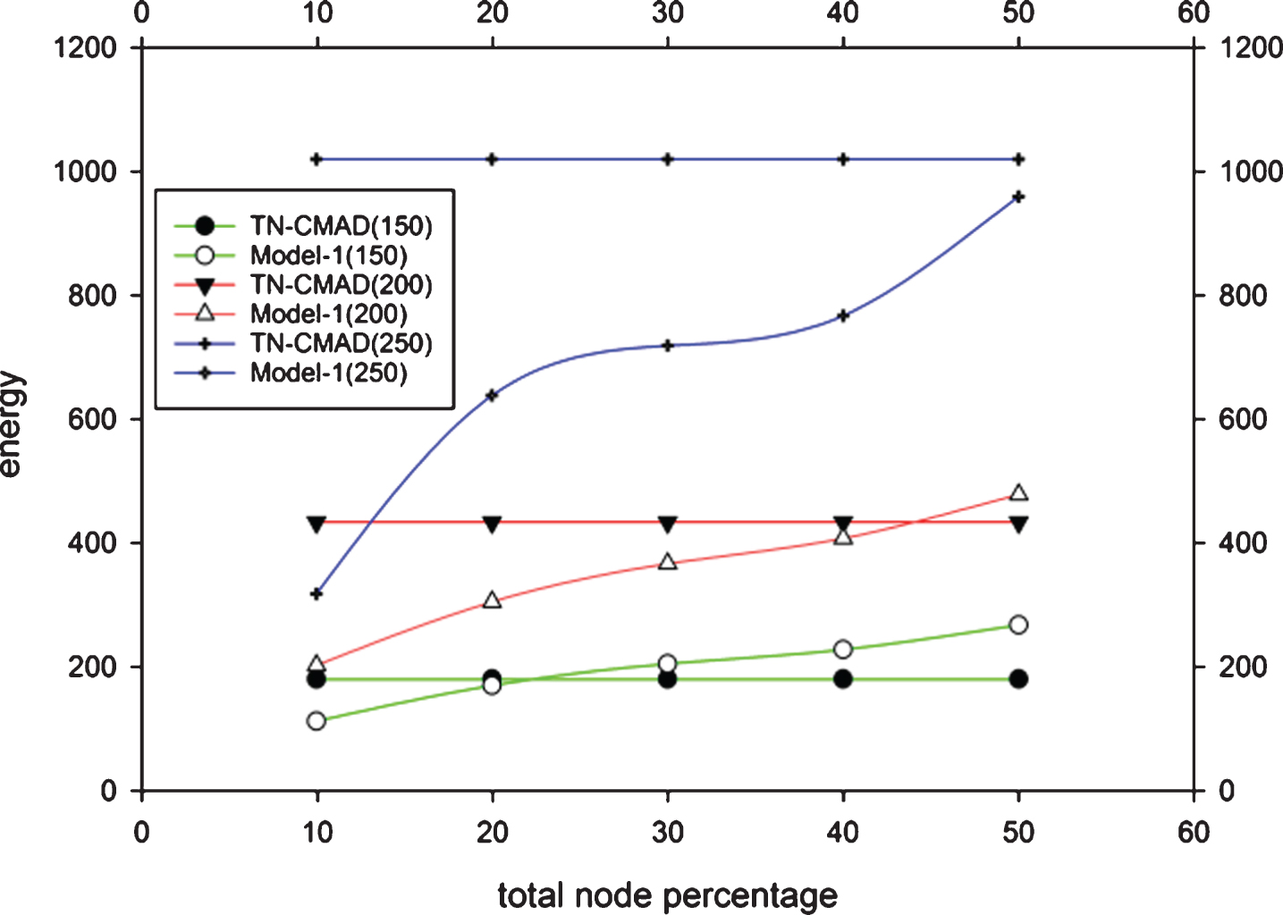
Overhead energy.

Within each time span of τ (4 seconds), overhead cost in TN-CMAD routing for a fixed transmission range is always fixed but in the proposed routing, overhead energy increases when more number of nodes send data packets within that time span. From simulation result it is found that for each R, Model-1 consumes lower overhead energy when node participation in data transmission is within a certain percentage of total nodes(23%, 40% and more than 50% when R is equal to 150, 200 and 250 units respectively) and as R increases performance of Model-1 gets better in terms of overhead energy.

We have checked lifetime of the links for LAR, LARDAR and compared with proposed models. The node speed are considered as 10 units/sec, 20 units/sec and 30 units/sec respectively. Simulation results are shown in Table 1. In second column, LL (Link lifetime) for LAR and LARDAR are shown and LL in our proposed models with the consideration of Equation (10) are shown in other columns. In the case of LAR and LARDAR Model, LL of both are same and have smaller value than our proposed models. In all cases LL of the network decreases with increase of speed of nodes and it is obvious. It is also found that LL for all three models are almost same.

Table 1

Link Life time of the Models in Sec

Velocity	LL	LL	LL
(unit/sec)	(LAR, LARDAR)	(Model-1,2)	(Model-3)
10	6.32	7.91	8.21
20	3.67	4.72	4.72
30	2.14	2.89	2.89

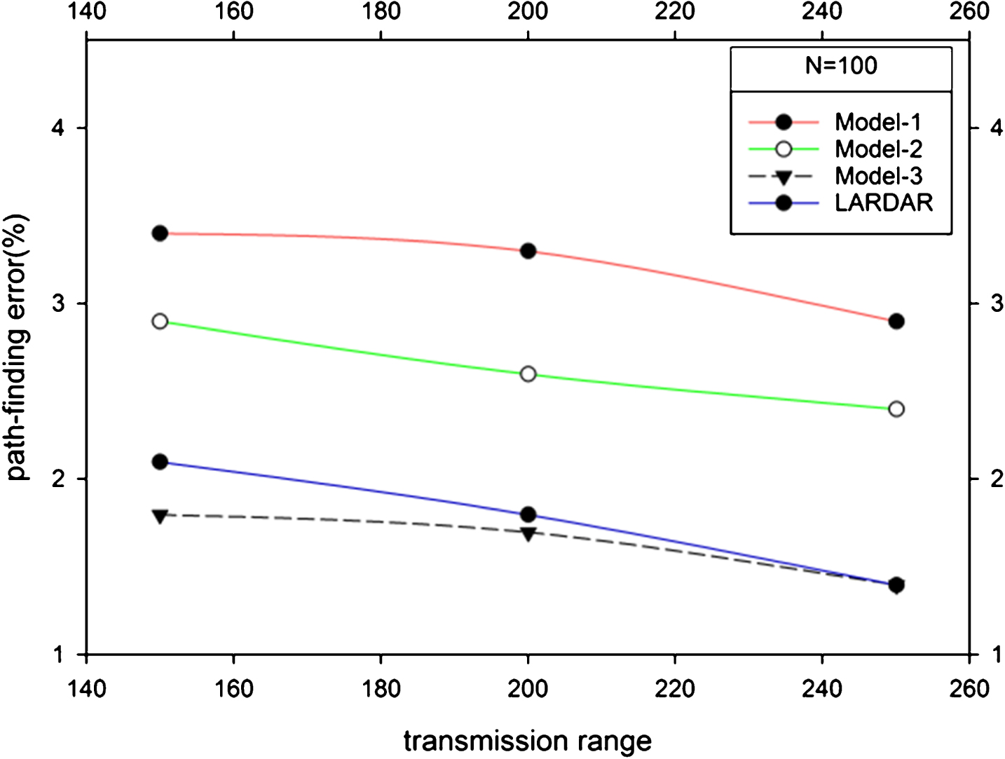
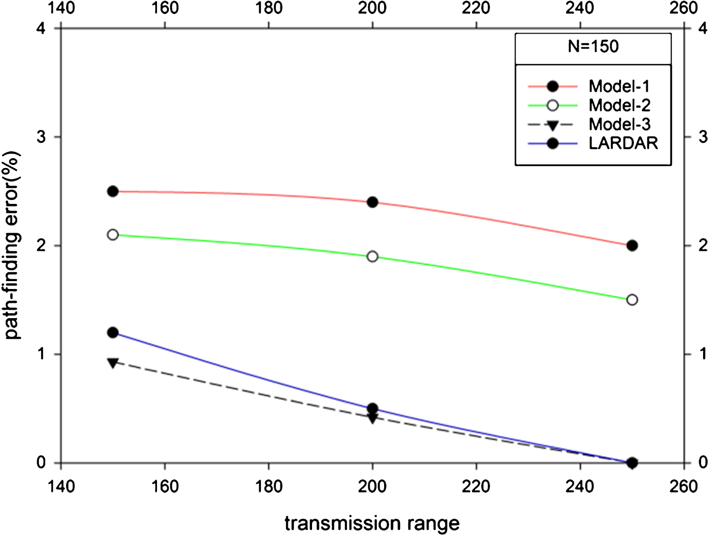
Finally we have compared our three models with LARDAR on the basis of path-finding error for different transmission range of the nodes. Path-finding error is an error when the route request packet may not reach the destination node due to unavailability of path from source to destination within the boundary of request zone. If θ in Fig. 4 is less than cut-off value, then it is called path-finding error. In Figs. 17–19, it is seen that as the request zone is larger for Model-1 compare to Model-2, the path-finding error is smaller for Model-1 relative to Model-2. But as we increase node density or transmission range, path-finding error decreases because with the increase of node density or transmission range, the availability of path to destination inside the request zone increases. LAR model has no path-finding error due to its large request zone but LARDAR

Fig. 17.

Path-finding error for node no 30.

Fig. 18.

Path-finding error for node no 40.

Fig. 19.

Path-finding error for node no 50.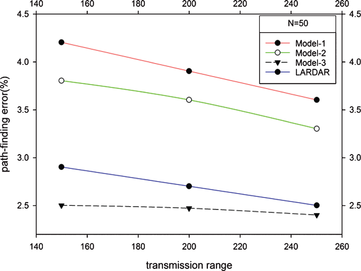

encounters path-finding error which is smaller than Model-1. Though our proposed models have path-finding error but percentage of error is very less, which has a very little impact on overall performance of the models, particularly the need of re-sending RREQ packets for route discovery.

In the second part of simulation, nodes are placed in an urban area and can move through available roads only. We have considered 100 nodes in the network and transmission range is considered as 100 unit. In all simulations we have chosen sender and receiver nodes randomly and based on different time interval between two successive transmission between sender and receiver, parameters like data overheads and distance travelled within the time span are being studied. We have also done simulation for LAR model on the same urban area network and compared with our proposed algorithm. As LAR has larger, rectangle shape request zone, it is thus most suitable for comparison with our model for urban area network. In Figs. 20, 21, time spans between two successive transmission towards same node are considered as 20 seconds and 30 seconds respectively and each simulation runs for 200 seconds. Requirement of overhead packets for sending a data after the time span is shown in the figures where it is found that overheads are increased with the increase of speed and have lower value when our proposed algorithm for urban area is used compared to the LAR. The cause of lower overheads is due to smaller expected zone of the receiver. Data overheads are also increased on increasing the time span between two successive transmission of the sender. It is due to increase of expected zone with the increase of time span.

Fig. 20.

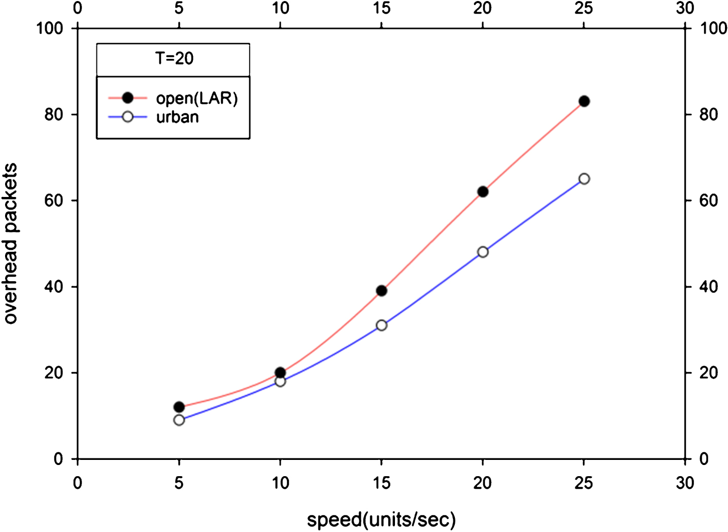
Overhead packets with varying velocity within time span 20 sec.

Fig. 21.

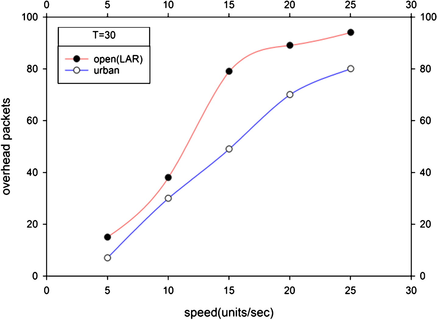
Overhead packets with varying velocity with time span 30 sec.

In Figs. 22, 23 we have also shown the distance travelled by receiver node from its earlier position within same time span of 20 and 30 sec. The distance calculated by using the proposed algorithm for urban area is always lower compare to LAR and it is increased with the increase of the node speed along with the time span of successive data transmission. Actual covered distance is also shown in the figures. As the actual travelled distance always lower than calculated values, thus during node discovery destination node is always be locatable.

6 Conclusion

In this paper we have considered four models which include three routing models for open area network and final model for urban area network. All the models have their different mobility pattern where parameters like node speed, direction of movement, pause time are being considered. In all models, considering the mobility pattern of nodes, we have proposed smaller cone shaped request zone which actually reduces the routing overhead and energy consumption in the network. Routing of MANET nodes in urban area is presented in separate section because the mobility of nodes are different compare to nodes in open field. we have shown, our proposed models used lesser number of overhead packets for route establishment and also consume smaller energy in comparision with routing model like LAR, LARDAR and TNCMAD. Finally it is also shown that the established paths always have longer life. But if the number of nodes decreses significantly, these models will suffer from hole problems and as result, routing performance will be degraded. Thus future work is to propose modified models which maintain good routing performance even in lower node density.

Fig. 22.

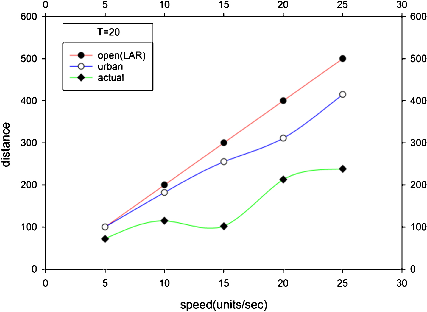
Distance covered with varying velocity within time span 20 sec.

Fig. 23.

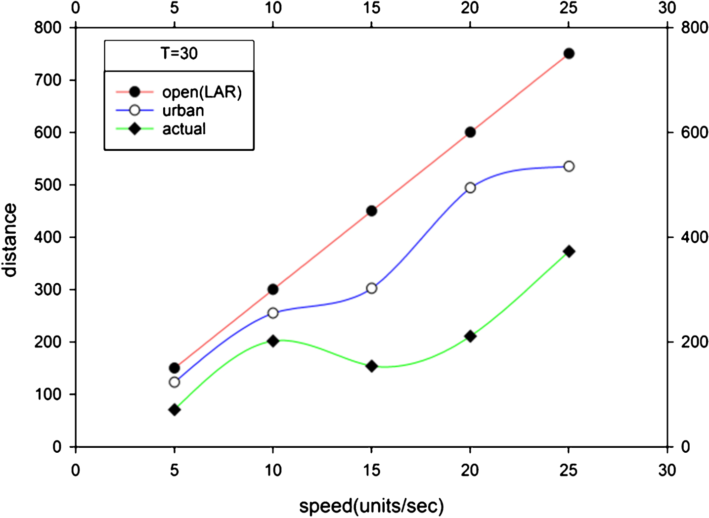
Distance covered with varying velocity within time span 30 sec.

References

Aboki ,

Shaghaghi ,

Akhlaghi and

Md Noor , Predictive location aided routing in mobile ad hoc network, In: Communications (MICC), 2013 IEEE Malaysia International Conference on, IEEE, 2013, pp. 57–61.

Basagni ,

Chlamtac ,

V.R.

Syrotiuk and

B.A.

Woodward , A distance routing effect algorithm for mobility (dream), In: Proceedings of the 4th annual ACM/IEEE international conference on Mobile computing and networking, ACM, 1998, pp. 76–84.

Chaki , Lar2p: A location aided reactive routing protocol for near-optimal route discovery in manet, In: 2010 International Conference on Computer Information Systems and Industrial Management Applications (CISIM), 2010, pp. 259–264, DOI 10.1109/CISIM.2010.5643654

Deb ,

S.B.

Roy and

Chaki , Lacber: A new location aided routing protocol for gps scarce manet, International Journal of Wireless & Mobile Networks (IJWMN)1(1) (2009), 22–34.

Dua ,

Kumar and

Bawa , A systematic review on routing protocols for vehicular ad hoc networks, Vehicular Communications1(1) (2014), 33–52.

K.T.

Feng and

T.E.

Lu , Velocity and location aided routing for mobile ad hoc networks, In: Vehicular Technology Conference, 2004. VTC2004-Fall. 2004 IEEE 60th, IEEE4 (2004), 2789–2793.

Haas and

Pearlman , The zone routing protocol: A hybrid framework for routing in ad hoc networks, (2001) ad hoc networking.

Hnatyshin ,

Ahmed ,

Cocco and

Urbano , A comparative study of location aided routing protocols for manet, In: Wireless Days (WD), 2011IFIP, IEEE (2011), 1–3.

Jacquet ,

Muhlethaler ,

Clausen ,

Laouiti ,

Qayyum and

Viennot , Optimized link state routing protocol for ad hoc networks, In: Multi Topic Conference, 2001. IEEE INMIC 2001. Technology for the 21st Century. Proceedings. IEEE International, IEEE, 2001, pp. 62–68.

10.

R.H.

Jhaveri and

N.M.

Patel , Mobile ad-hoc networking with aodv: A review, International Journal of Next-Generation Computing6(3) (2015).

11.

D.B.

Johnson , The dynamic source routing protocol for mobile ad hoc networks, (2003). draft-ietf-manet-dsr-09 txt

12.

Junyan ,

Cheng ,

Huagang and

Youzi , An efficient location-aided link state routing protocol for manets, In: Information Science and Engineering (ICISE), 2010 2nd International Conference on, IEEE, 2010, pp. 1827–1830.

13.

Y.B.

Ko and

N.H.

Vaidya , Location-aided routing (lar) in mobile ad hoc networks, Wireless Networks6(4) (2000), 307–321.

14.

H.C.

Liao and

C.J.

Lin , A position-based connectionless routing algorithm for manet and wimax under high mobility and various node densities, Information Technology Journal7(3) (2008), 458–465.

15.

Mauve ,

Widmer and

Hartenstein , A survey on position-based routing in mobile ad hoc networks, Network, IEEE15(6) (2001), 30–39.

16.

Meghanathan , Location prediction based routing protocol for mobile ad hoc networks, In: Global Telecommunications Conference, 2008. IEEE GLOBECOM 2008. IEEE (2008), 1–5. IEEE.

17.

M.A.

Mikki , Energy efficient location aided routing protocol for wireless manets (2009), arXiv preprint arXiv:09090093

18.

Nagwani and

D.S.

Tomar , Mobility prediction based routing in mobile adhoc network using hidden markov model, International Journal of Computer Applications59(1) (2012).

19.

C. Perkins, E. Belding-Royerand S. Das, Ad hoc on-demand distance vector (aodv) routing, Tech. rep.

20.

Phoummavong ,

Utsu ,

C.O.

Chow and

Ishii , Location-aided route discovery mechanism based on two-hop neighbor information for ad hoc network, The Journal of Supercomputing72(3) (2016), 1201–1214.

21.

Quintero ,

Castro , et al., A location routing protocol based on smart antennas for ad hoc networks. Journal of Network and Computer Applications30(2) (2007), 614–636.

22.

A.G.

Shaji ,

Hemrajani and

Kaushik , Energy aware multipath location aided routing for manet, International Journal of Computer Science and Information Security14(12) (2016), 308.

23.

T.F.

Shih and

H.C.

Yen , Location-aware routing protocol with dynamic adaptation of request zone for mobile ad hoc networks, Wireless Networks14(3) (2008), 321–333.

24.

Vijayakumar and

Ravichandran , Efficient location management of mobile node in wireless mobile ad-hoc network, In: Innovations in Emerging Technology (NCOIET), 2011 National Conference on, IEEE (2011), 77–84.

25.

Yi ,

Liang ,

Xinyu and

Zhang , Cluster based location-aided routing protocol for large scale mobile ad hoc networks, IEICE Transactions on Information and Systems92(5) (2009), 1103–1124.

26.

Kalaivani ,

Sathya and

Senthilnathan , Dynamic Data Routing in manet using position based opportunistic Routing Protocol, International Journal of research in computer Applications & Robotics (IJRCAR)2 (2014), 12.

27.

K.D.

Lakshmi and

Ramesh , Energy efficient position based opportunistic routing protocol for MANETS, International Journal of Computer Science andNetwork Security (IJCSNS)14(6) (2014), 31.

28.

N.S.

Kavitha ,

Malathi ,

J.M.

Philip and

Pravinth Raja , Performance analysis of efficient position-based opportunistic routing for MANET. In: Shetty N., Patnaik L., Prasad N., Nalini N. (eds), Emerging Research in Computing, Information, Communication and Applications. ERCICA2016 (2018), Springer, Singapore.

29.

R.R.

Colletti and

R.M.

de Moraes , Evaluation of link lifetime for the random waypoint mobility model, Networks (ICON)2013 19th IEEE International Conference on, 2013, pp. 1–5.

30.

Pramanik ,

Choudhury ,

T.S.

Choudhury ,

Arif and

Mehedi , Behavioral study of Random Waypoint Mobility Model based energy aware MANET. In Signal Processing and Integrated Networks (SPIN), 2016 3rd International Conference on, IEEE, 2016, pp. 624–629.