Exploiting abstract change pattern from code changes

The abstractly context-aware change pattern P is exploited from many concrete code changes with the ACP abstracting algorithm. Algorithm 1 describes this process procedurally in the six steps.

Step 1: Obtaining changes

Let M = {m₁, ⋯, m _i }. m _i is the ith original source code. Let M^′= {m₁’, ⋯, m _i ’}. m _i ’ is the changed version of m _i . For the source code m _i , we represent it with Abstract Syntax Tree (AST _i ), characterize code changes as AST changes Δ _i given by Δ _i = {e _i | e _i ∈ delete(u,v,k), insert(u,v,k), move(u,v,k), update(u,v)}.

Insert (node u, node v, int k): insert u and position it as the (k+1)-th child of v;

Delete (node u, node v, int k): delete u at the (k+1)-th child of v;

Update (node u, node v): replace the label and AST type of u with v while maintaining u’s position;

Move (node u, node v, int k): delete u from its current position and insert it as the (k+1)-th child of v.

Let m _i  + Δ _i  = m _i ’. It implies that source code m _i undergoes the changes Δ _i and becomes a new source code m _i ’. These code changes are obtained with Distiller [12], such that Δ _i  = m _i ’-m _i . Distiller computes the one-to-one node mapper between the versions of m _i ’s AST before and after changes.

In our example, the original methods m _A , m _B and the changed source code m _A ’, m _B ’ are transformed into AST _A , AST _A ’ and AST _B , AST _B ’ as shown in Fig. 2, where ^′O^′ represents the nodes in m _A and m _B while ^′N^′ represents the nodes in m _A ’ and m _B ’. Each node corresponds to each line of code statement in Fig. 1. For example, O₆ in AST _A corresponds to ^″MVAction action = (MV Action)e.next();^″ in m _A . N₄ in AST _A ’ corresponds to ^″object next = e.next();^″ in m _A ’.

OPEN IN VIEWER

Fig.2

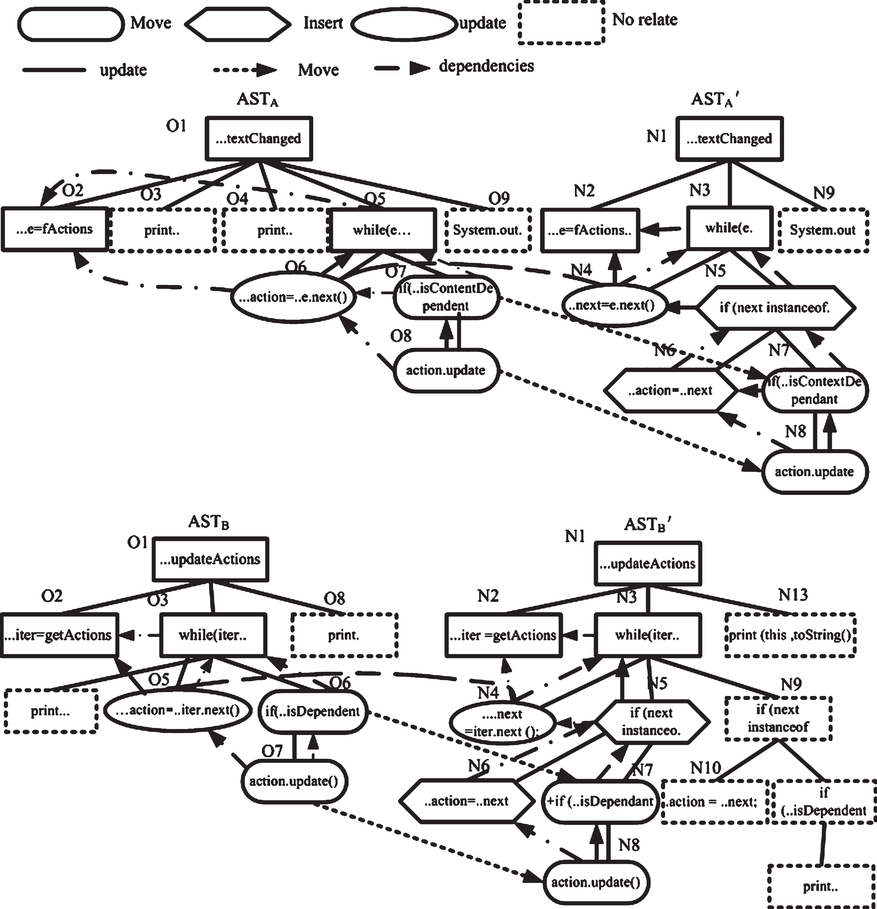
AST comparing analysis for m _A and m _B .

The code changes (Δ _A , Δ _B ) of the source code (m _A , m _B ) are obtained as follows:

Δ _A  = {e _{A 1} (Delete 0₃ 0₁ 1), e _{A 2} (Delete 0₄ 0₁ 2), e _{A 3} (Move 0₅N₁ 1), e _{A 4} (Update 0₆N₄), e _{A 5} (Move 0₇N₅ 1), e _{A 6} (Move 0₈N₇ 0), e _{A 7} (InsertN₅N₃ 1), e _{A 8} (InsertN₆N₅ 0)};

e _{A 1} refers to deleting 0₃ at the second child of 0₁, corresponding to the deletion (m _A : line 3) inFig. 1;

e _{A 4} refers to replacing the label and AST type of 0₆ with N₄ while maintaining 0₆’s position in the tree, corresponding to the update (m _A : line 6) inFig. 1;

e _{A 5} refers to deleting 0₇ from its current position and insert it as the second child of N₅, corresponding to the move (m _A : line 7) in Fig. 1;

e _{A 7} refers to inserting N₅ and position it as the second child of N₃, corresponding to the insertion (m _A ’: line 5^′) in Fig. 1.

In the same way, Δ _B = {e _{B 1} (Delete 0₄ 0₃ 1), e _{B 2} (Update 0₅N₄), e _{B 3} (Move 0₅N₃ 0), e _{B 4} (Move 0₆N₅ 1), e _{B 5} (Move 0₇N₇ 0), e _{B 6} (InsertN₅N₃ 1), e _{B 7} (InsertN₆N₅ 0), e _{B 8} (InsertN₉N₃ 2), e _{B 9} (InsertN₁₀N₉ 0), e _{B 10} (InsertN₁₁N₉ 1), e _{B 11} (InsertN₁₂N₁₁ 0)}.

Step 2: Identifying common changes

The common changes Δ _c are identified with the modified Longest Common Edit Operation Subsequence (LCEOS) algorithm [13]. The algorithm iteratively compares the node operations in Δ _i pairwise, such that Δ c = ⋂ i = 1 n Δ _i , ∀1≤ i ≤ n, Δ _{c i} ⊆ Δ _i , in which the threshold t _s  = 0.6 is used to tolerate the inexact matches between the node operations pair. If it fails to find any identical node operations in the pair, it converts all concrete instances of types, methods and variables in node operations to the abstract identifiers $t, $m and $v. If these abstract identifiers have the same edit type or inheriting type but the different representations of the label, they are still abstractly equivalent. Thus the result of the matching is a list of common changes Δ _c .

In our example, the longest common changes are identified as follows: Δ _c  = {pair₁ (e _{A 4} , e _{B 2} ), pair₂ (e _{A 5} , e _{B 4} ), pair₃ (e _{A 6} , e _{B 5} ), pair₄ (e _{A 7} , e _{B 6} ), pair₅ (e _{A 8} , e _{B 7} )}, which refers to {updates (m _A : line 6), insertions (m _A ’: line 5^′– 6^′), moves (m _A : line 7–8)} and {updates (m _B : line 5), insertions (m _B ’: line 5^′– 6^′), moves (m _B : line 6–7)}, as shown in Fig. 1.

Step 3: Generalizing abstract changes

Comparing the node operations in Δ _c pairwise, the abstract changes are generalized, which are applicable to any target source code with the different identifiers. In these node operation pairs, if one or more concrete instances of types, methods and variables have the same edit type or inheriting type, but the different name, these instances are abstractly equivalent. Then the abstract identifiers $t, $m and $v are substituted for these concrete instances in both node operation pairs and the method itself. Meanwhile, the mapper between the identifiers and the concrete instances are recorded. To enforce a consistent naming, if some subsequent node operation pairs are inconsistent with the current mapper, they are omitted. Algorithm 2 describes the whole process.

In our example, e _{A 4} (Update 0₆N₄) matches with e _{B 2} (Update 0₅N₄) in pair₁ (e _{A 4} , e _{B 2} ). The discrepant variable names e vs. iter are detected. The identifiers mapper (e, $v₁) and (iter, $v₁) are recorded, which substitutes a fresh abstract identifier $v₁ for e in e _{A 4} (Update 0₆N₄), m _A (O₂, O₅, O₆), m _A ’ (N₂, N₃, N₄), as well as iter in e _{B 2} (Update 0₅N₄), m _B (O₂, O₃, O₅), m _B ’ (N₂, N₃, N₄). pair₂ (e _{A 5} , e _{B 4} ) does so as well. The identifiers mapper {(isContentDependent, $m₁) (isDependent, $m₁)} are recorded, which substitutes $m₁ for isContentDependent in e _{A 5} (Move 0₇N₅ 1), m _A (O₇) as well as all isDependent in e _{B 4} (Move 0₆N₅ 1), m _B  (O₆).

Step 4: Extracting changes-relevant context

Let C = {c _i |c _i ∈ DataDepend (x,y), ControlDepend (x,y), ContainDepend (x,y)}. c _i is the changes-relevant context of m _i while contains the unchanged nodes of AST _i ’ on which changed nodes in e _i . The context increases the chance of generating the valid changes syntactically and also serves as the anchors to position changes correctly in a new target location.

Formally, the node y depends on the node x if one of the following relationships holds:

DataDepend (node x, node y): the node x uses or defines a variable whose value is defined in thenode y.

ControlDepend (node x, node y): the node y is control dependent on the node x if y may or may not execute depending on a decision made by x. Formally, given a control-flow graph, y is control dependent on x, if: (i) y post-dominates every vertex p in x ⇝ y, p ≠ x and (ii) y does not strictly post-dominate x.

ContainDepend (node x, node y): the node y is containment dependent on the node x if y is a child of x in the AST.

The changes-relevant context c _i of the method m _i is extracted with the control, data and containment dependence analysis. All irrelevant nodes are omitted because blindly including the irrelevant nodes as context puts the unnecessary constraints on the potential change locations and results in the false negatives during change location search. Then the node positions are recalculated in AST _i and Δ _i .

In our example, as shown in Fig. 2-AST _A , we consider (i) e _{A 7} (Insert N₅N₃ 1): The inserted node N₅ is control dependent on N₃ and data dependent on N₄ and N₂. Mapping these nodes to the old version yields the context nodes {O₂, O₅, O₆}; (ii) e _{A 5} (Move O₇N₅ 1): The moved node O₆ depends on the nodes c₁ = {O₂, O₅, O₆} in the m _A , while N₇, N₅’s child at position 1, depend on the nodes c₂ = {N₂, N₃, N₄, N₅} in the new m _A ’; (iii) the other changes do so as well. After extracting context, irrelevant nodes with dotted lines are omitted, such as {O₃, O₄, O₉} in AST _A and N₉ in AST _A ’. Then the node position are reset in AST _A and AST _A ’.

Step 5: Generalizing abstract contexts

Using the LCEOS algorithm [13], the common contexts C _c are identified by iteratively comparing the node operation in c _i pairwise, such that C c = ⋂ i = 1 n c _i , ∀1≤ i ≤ n, c _{c i} ⊆ C _i . Then the node operations in C _c pairwise are compared iteratively to generalize the abstract contexts, as does step 3.

In our example, the common contexts are identified, such as pair₃(m _A (O₂), m _B (O₂)), pair₄ (m _A (O₅), m _B (O₃)). Then the same for the pair₃ (m _A (O₂), m _B  (O₂)) is done as step1-B to generalize the abstract contexts. The identifiers mapper {(fAction,$m₂), (getAction, $m₂)}, are recorded, and $m₂ is substituted for fActions in m _A (O₂) and getActions() m _B  (O₂).

Step 6: Generating the context-aware change pattern

All common contexts C _c are merged into an abstract changes-relevant context C. In our example, C is described as follow:

public void method declaration (⋯){

All the common changes Δ _c are merged into an abstract changes Δ. In our example, Δ is described as follow:

Update O₄N₄

   O₄ = ′MVAction action = (MVAction) $v1.next();^′

   N₄ = ′object next = $V1.next;^′

Move O₅N₅ 1O₅ = ′if(cation.$m1())^′

Move O₆N₇ 0 O₆ = ′action.update()^′

Insert N₅N₃ 1 N₅ = ′if (next instance of MVAction)^′

Insert N₆N₅ 0 N₆ = ′MVAction action =(MVAction) next^′

C and Δ are combined into the abstractly context-aware change pattern P, such that P (C, Δ). The P implies that the source code C undergoes the changes Δ and becomes a new source code C’, such that C +Δ= C’, as shown in Fig. 3.

OPEN IN VIEWER

Fig.3

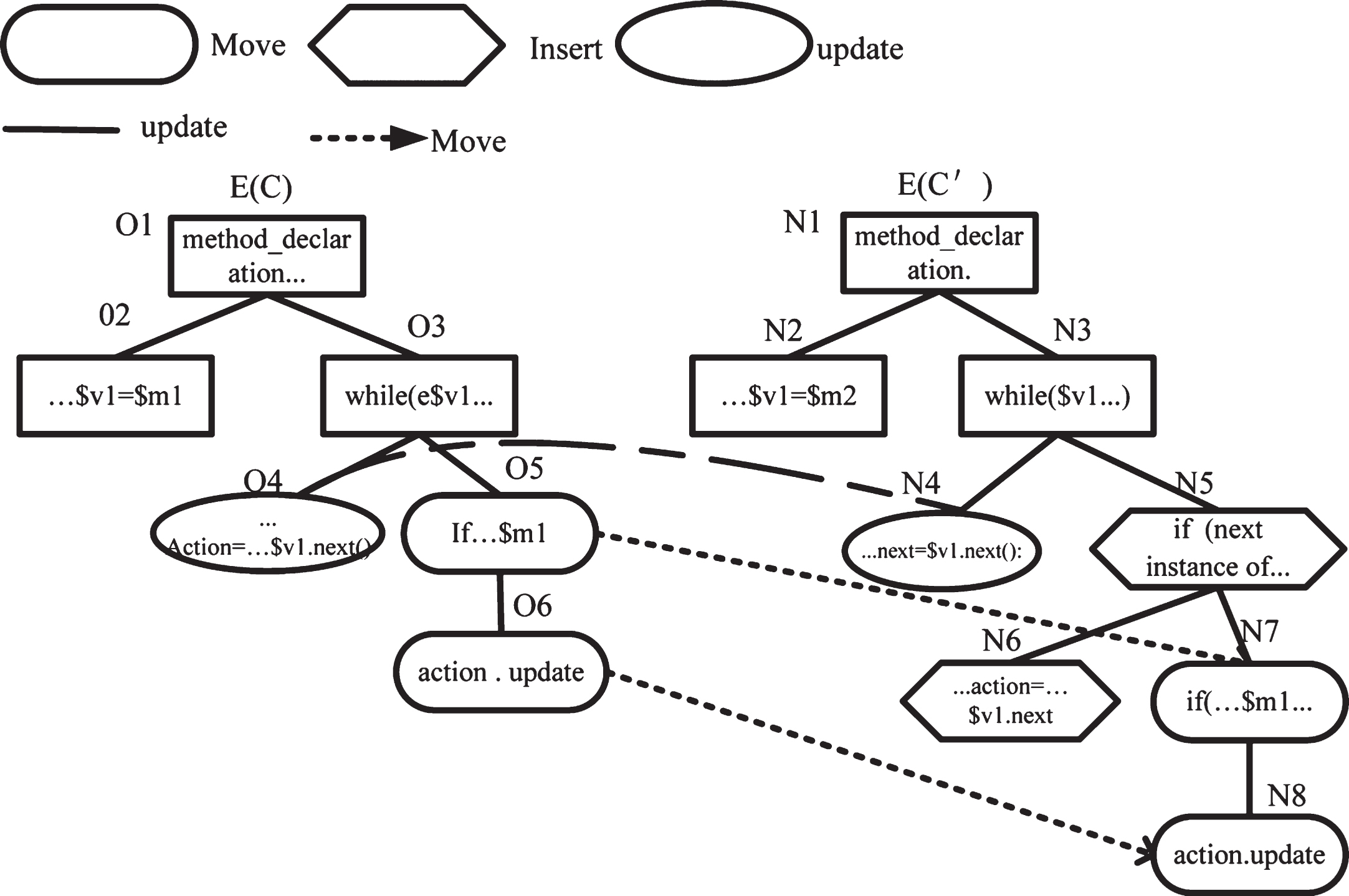
The mechanism of change pattern.

Based on the abstractly context-aware change pattern P, the target source code m are changed automatically by producing mapping, customizing the concrete changes and replicating the changes on m. Algorithm 3 describes this process procedurally in three steps.

Step1: Producing nodes/identifiers mapper

For target method m and the abstract context C of the abstractly context-aware change pattern P, with Matching Abstract Context to Target Tree [14, 15], the nodes mapping is established by finding the nodes in m that match the nodes in C, and induces the one-to-one identifiers mapper between the abstract identifiers in C and the concrete identifiers in m. In this process, if every node in C has a match in m, the concrete changes are derived to customize m. If no match for each node is found, it reports the change pattern cannot replicate the changes on m.

In our example, the nodes mapping (C, m _C ) = {(1, 1), (2, 2), (3, 3), (4, 4), (5, 5), (6, 6)} and the instances/identifiers mapper {($v₁, e). ($m₁,isSelectionDependent), ($m₂, fActions)} are established by matching the nodes between C and AST _c .

Step 2: Customizing the concrete changes script

All abstract identifiers in the abstract changes Δ are replaced with the corresponding concrete names of the target source code m based on the instances/identifiers mapper. Then the node positions of Δ are recalculated with respect to the concrete nodes in m.

In our example, the concrete changes Δ _c for m _c are customized based on the instances/identifiers mapper. $v₁, $m₁(), $m₂() are substituted for all instances of e, isSelectionDependent (), fActions in Δ, as follows:

Update O₄N₄

   O₄=^′MVAction action = (MVAction) $v1.next();^′

   N₄=^′object next = e. next ();^′

Move O₅N₅ 1O₅ = ′if (cation.isSelectionDependent())^′

Move O₆N₇ 0 O₆ = ′action.update();^′

Insert N₅N₃ 1 N₅ = ′if (next instance of MVAction);^′

Insert N₆N₅ 0 N₆ = ′MVAction action =(MVAction) next;^′

Setp 3: Changing the target method

With Δ _m ’ the target method m is transformed to the source code m^′ meeting user needs, such that m +Δ _m = m^′. In our example, instead of Jim’s manual changes, the update (m _c : line 4), the insertions (m _c ’: line 5^′– 6^′) and the moves (m _c : line 5–6) are applied to m _c to instead achieve the motivating hypothesis described as shown in Fig. 1 (m _c ).

Experiment-A: We collect 7 topics, each topic has many different code snippets replied by users. From the code changes of these code snippets, ACPM exploits the change pattern about this topic. Based on the change pattern ACPM could transform other different code snippet of the same topic. The accuracy helps us evaluate whether ACPM ensures the context-specific code is general for the various contexts or not.

However, Table 1-A shows the opposite results with T₁ (35%), T₂ (34.37%), T₄ (35%), T₆ (33.75%) and T₇ (33.56%), but a few promising results with T₃ (80.6%), T₅ (78.6%). To analyze the reason for these results, we explore how sensitive ACPM is to the similarity and the number of code snippets.

We depict the poor results (T₁, T₂, T₄, T₆ and T₇ in Table 1-A). The accuracy goes down as shown in Fig. 4(a). It illustrates that the more code snippets provided, the less similar code snippets are, the less context is likely to be shared among them. Exploiting from multiple code snippets has the lower accuracy when suggesting changes for correctly identified locations. Because using multiple code snippets reduces the common changes, the derived change is likely to be less accurate for any one target location.

OPEN IN VIEWER

Fig.4

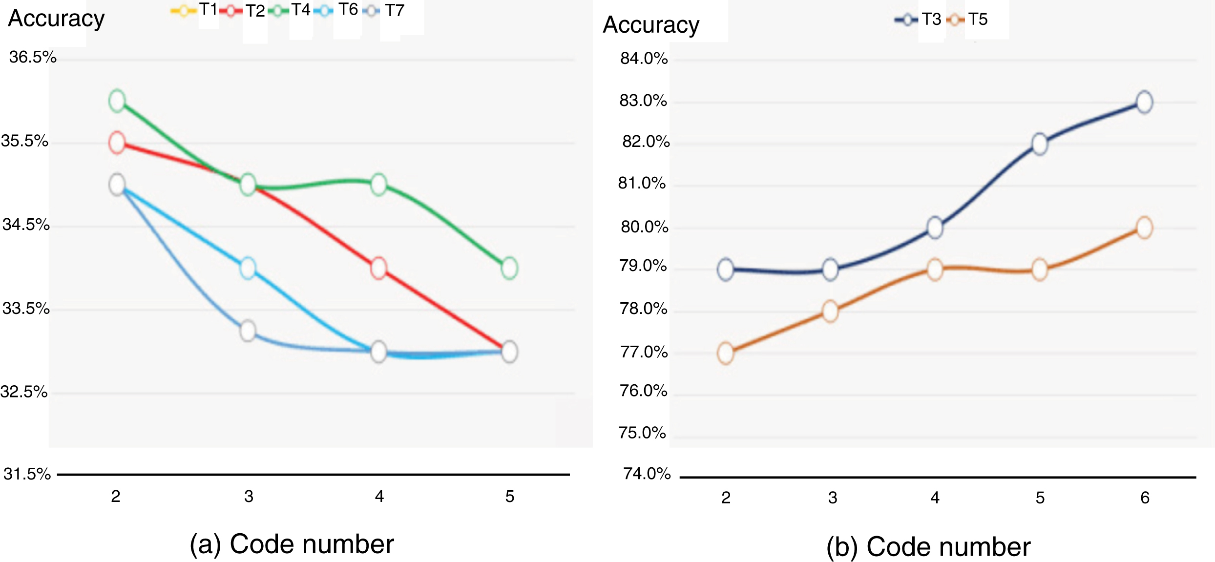
The analysis of the poor or good results.

We depict the promising results (T₃ and T₅ in Table 1-A) as shown in Fig. 4(b). The accuracy can go up when more code snippets are given, which is different from Fig. 4(a). It illustrates the accuracy can vary inconsistently with the number of code snippets, because it strictly depends on the similarity of code snippets. For instance, when code snippets are diverse, ACPM extracts the fewer common changes which decrease the accuracy. When code snippets are similar, adding code snippets may not decrease the number of common changes, but induce more identifier abstraction and generate the more flexible changes to increase the accuracy.

In sum, if code snippets are different, T₁, T₂, T₄, T₆ and T₇ in Table 1-A occurs, otherwise T₃ and T₅ in Table 1-A occurs. From these results, a sensitivity-related rule (1) is found: the accuracy varies with the similarity and the number of code snippets, while the similarity taking precedence over the number. The more similar code snippets are, the more code snippets given, the higher accuracy is.

To improve the above poor results (T₁, T₂, T₄, T₆ and T₇ in Table 1-A), we change the experiment-A to the experiment-B according to the rule (1). We pick the representative code snippet outs of all snippets. Then ACPM exploits the change pattern from the code changes of the representative code snippets instead of all code snippets. Because the similarity between the different versions of the same code snippet is higher than the similarity between the different code snippets.

In the experiment-A, let m _i  + Δ _i  = m _i ’, the source code m _i undergoes the changes Δ _i and becomes a new source code m _i ’. Δ _i is the changes of the different source code m _i . For example, Δ₁ is the changes of the first source code m₁. Δ _i is the changes of the second source code m₂. In the experiment-B, let m_i-1 + Δ _i  = m _i ’ instead of m _i  + Δ _i  = m _i ’. Each source code has many changed version. Δ _i represents the changes between the current changed version and the last changed version, such that Δ _i  = m _i ’– m_i-1. For example, Δ₁ is the first changes of the source code m. Δ₂ is the second changes of the changed source code m₁. Note that the ^″num^″ column in Table 1 represents the number of different versions of the representative code snippet. To evaluate whether the accuracy of T₁, T₂, T₄, T₆ and T₇ raise or not, we conduct experiment B. Table 1-B shows the better results with T₁ (63.75%) and T₇ (63.5%) than the ones in Table 1-A.

4.3 The effect of the stable change pattern

In Table 1-B, the accuracy of T₂ is still 0 because every new changes is the addition of the last changes. Suppose that first only m exists, then m₁ = m + Δ₁, next m₂ = m + Δ₁ + Δ₂, finally m₃ = m + Δ₁ + Δ₂ + Δ₃ and Δ₁ ≠ Δ₂ ≠ Δ₃, such that (m₁ - m) ⋂ (m₂ - m₁) ⋂ (m₃ - m₂) = Δ₁ ⋂ Δ₂ ⋂ Δ₃ = Φ, ACPM decides there is no common changes.

To improve it, we change the experiment-B to the experiment-C. In the experiment-C, let Δ _i  = m _i ’-m instead of Δ _i  = m _i ’– m_i-1. Δ _i represents the different changes of the same source code m. For example, Δ₁ is the first changes of the source code m. Δ₂ is the second changes of the same source code m. In this case, T₂ supposes that (m₁– m) ⋂ (m₂ - m)⋂ (m₃ - m) = Δ₁ ⋂ (Δ₁ + Δ₂) ⋂ (Δ₁ + Δ₂ + Δ₃) = Δ₁, ACPM decides that there are common changes Δ₁.

To evaluate whether T₂ restore or not, we conduct the experiment-C. Table 1-C shows T₂ recovers from 0% to 69.18% and T₁, T₇ are also a little better than the ones in Table 1-B.

4.4 The effect of the first modification

In Table 1-C, the accuracy of T₄ is still 0. We discover each changes Δ _i is similar except the first changes Δ₁. Because Δ₁ involves amounts of changes to fix bugs while other subsequent Δ _i involves small changes unrelated to bugs. In this case, Δ₁ is a outlier such that Δ _outlier  ⋂ ∀ Δ _i  = Φ.

To evaluate whether T₄ restore or not, we change the experiment-C to the experiment-D. We identify the common changes Δ _c starting from Δ₂ instead of Δ₁, such that Δ c = ⋂ i = 2 n Δ _i and conduct the experiment-D. Table 1-D shows T₄ recovers from 0% to 71.18% and T₁, T₂, T₇ are also a little better than the ones in Table 1-C. It illustrates ACPM is not only sensitive to the similarity of code snippets m _i , but also sensitive to the similarity of Δ _i .

4.5 The effect of the similar changes

To explore how sensitive ACPM is to the similarity of Δ _i , we re-focus in Table 1-B. we (i) depict the result of T₁ as Fig. 5(a-T₁) where the accuracy still decreases because no Δ _outlier exists; (ii) depict the result of T₄ as Fig. 5(a-T₄) where the accuracy decreases to 0 suddenly at the second changes and never goes up again because Δ₁ is a outlier; (iii) depict the result of T₆ as Fig. 5(a-T₆) where the accuracy decreases to 0 suddenly at the forth changes because Δ₄ is a outlier. In sum, the accuracy decreases as the number of Δ _i . Sometimes, it decreases suddenly to 0 and never restores if Δ _outlier exists. Thus the second sensitivity-related rule (2) is the more similar changes Δ _i are, the higher accuracy is.

OPEN IN VIEWER

Fig.5

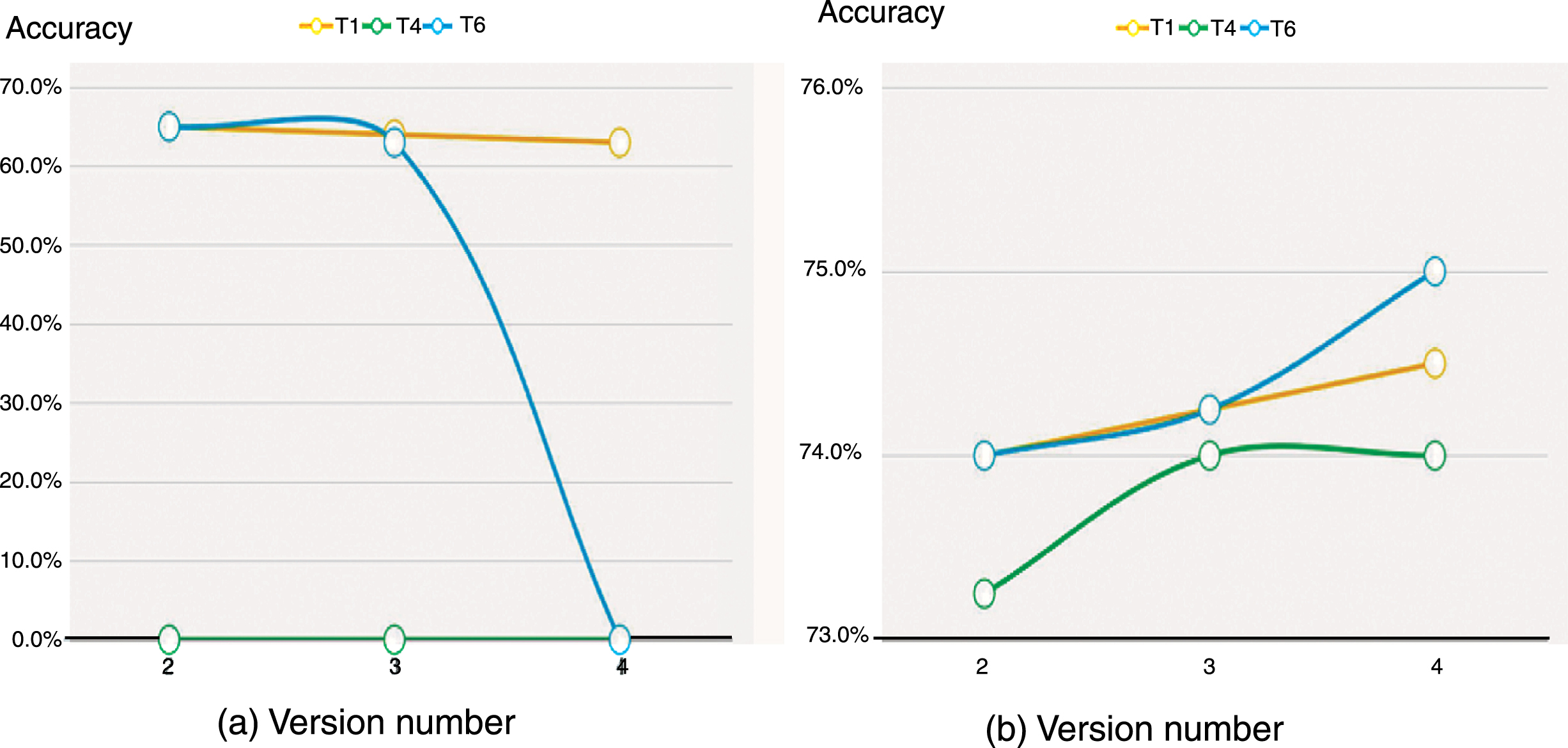
The before and after heuristic strategy.

To avoid ill-effects of Δ _outlier , such as a sudden decrease, we change the experiment-D to the experiment-E. We design a heuristic changes-choosing strategy to choose the top-N similar Δ _i with the largest intersection and exclude Δ _outlier actively. N represents as the maximum number of the common changes Δ _c . Suppose that N = 2, Δ₁ occurs, Δ _c  = Δ₁; next Δ₂ occurs, Δ _c  = Δ₁ ⋂ Δ₂; then Δ₃ occurs, if Δ₁ ⋂ Δ₂ ≠Φ, Δ₁ ⋂ Δ₃ = Φ and Δ₂ ⋂ Δ₃ = Φ, we choose Δ _c  = Δ₁ ⋂ Δ₂ as the largest intersection and omit Δ₃; go on Δ₄ occurs, if (Δ₁ ⋂ Δ₄) > ((Δ₁ ⋂ Δ₂) or (Δ₂ ⋂ Δ₄)), we choose Δ _c  = Δ₁ ⋂ Δ₄ and omit Δ₂, and so on.

We conduct the experiment-E with the default setting of 2 for N. Surprisingly, Table 1-E shows T₆ decreased to 0 at the fourth changes previously but now it still increases, while T₄ decreased to 0 at the second changes previously but now it also still increases, even recovers from 34.81% to 74.56% averagely. T₁, T₂, T₄, T₇, T₈ are also a little better than the ones in Table 1-D.

Besides in Table 1-E, we (i) depict the result of T₁ as Fig. 5(b-T₁) where the accuracy still increases as the number of code snippets; (ii) depict the result of T₄ as Fig. 5(b-T₄) where the accuracy decreases to 0 suddenly at the second changes and goes up again despite a outlier Δ₁; (iii) depict the result of T₆ as Fig. 5(b-T₆) where the accuracy still increases despite a outlier Δ₄. In sum, the heuristic changes-choosing strategy makes sense that no matter how many times the code snippet is changed, the accuracy still remains or increases as the number of Δ _i or recovers soon despite sudden decreasing immediately to 0 at the second changes.