An analysis of consensus approaches based on different concepts of coincidence

Abstract

Soft consensus is a relevant topic in group decision making problems. Soft consensus measures are utilized to reflect the different agreement degrees between the experts leading the consensus reaching process. This may determine the final decision and the time needed to reach it. The concept of coincidence has led to two main approaches to calculating the soft consensus measures, namely, concordance among expert preferences and concordance among individual solutions. In the first approach the coincidence is obtained by evaluating the similarity among the expert preferences, while in the second one the concordance is derived from the measurement of the similarity among the solutions proposed by these experts. This paper performs a comparative study of consensus approaches based on both coincidence approaches. We obtain significant differences between both approaches by comparing several distance functions for measuring expert preferences and a consensus measure over the set of alternatives for measuring the solutions provided by experts. To do so, we use the nonparametric Wilcoxon signed-ranks test. Finally, these outcomes are analyzed using Friedman mean ranks in order to obtain a quantitative classification of the considered measurements according to the convergence criterion considered in the consensus reaching process.

Keywords

Group decision making fuzzy preference relations consensus

1 Introduction

A group decision making (GDM) problem ends when the experts choose among a set of alternatives those ones that will be a solution. Usually, together with the solution obtained, it is convenient to know the degree of agreement reached by these experts [8, 18 , 54].

Facing the classical notion of consensus as a full agreement among individuals that form a group of decision -experts-, Kacprzyk et al. [21 , 24] introduce the concept of soft consensus to model the agreement process in GDM problems. This concept allows the definition of soft consensus criteria which are the basis of numerous consensus approaches [1, 33 , 53]. In such a way, consensus measures assessed in [0,1] are introduced, where 0 means null consensus, 1 means total consensus, and values in (0,1) mean diverse partway consensus situations [4 , 19]. Then, a process of reaching consensus could be established as a multistage process iteratively developed and made up of several discussion and consensus rounds [12 , 20]. In each round we consider the existence of a coordinator of the process -moderator-, who evaluates the consensus levels existing among the experts through soft consensus measures. Fixed a particular consensus threshold, a consensus level is less than that threshold means that a large discrepancy among experts’ opinions is observed. In such a case, the coordinator would propose that the experts discuss their opinions so as to make them closer. In the case that an acceptable consensus level has been reached, it could be possible to make use of a selection process so as to get the ending solution [4 , 19].

Given a set of alternatives in a GDM problem, experts can express their preferences in different ways such as: fuzzy preference relations [12 , 23], multiplicative preference relations [20, 45], linguistic preference relations [1 , 39], hesitant fuzzy preference relations [46, 47] or intuitionistic fuzzy preference relations [27–29 , 50].

In addition, different approaches to consensus can be considered according to different criteria [4 , 19]. One of this criterion is the coincidence among the experts’ preferences. In this case, soft consensus measures act on the preferences expressed by the experts, and consequently, their computation is build around the concept of similarity among preferences [4 , 19]. We should point out that the specific metric (distance function) utilized to assess the similarity could influence the convergence of the consensus processes so as to get a solution admissible by the majority of experts. Another criterion is the coincidence among the solutions expressed by the experts. In this case, the coincidence is computed by comparing the positions of the alternatives observed in the individual solutions and the collective solution. We should point out that this coincidence approach provides a more realistic measure of consensus among experts [19, 20].

In this paper we use frequently employed fuzzy preference relations that we have already handled in previous papers [12, 20] to analyze the behavior of the two aforementioned consensus approaches in GDM problems. We present a comparative study between both approaches. Two-sample statistical tests are used to study the differences among five of the distance functions most commonly used in modelling soft consensus in GDM problems: Manhattan, Euclidean, Cosine, Dice, and Jaccard distance functions [12], and the consensus measure over the set of alternatives called C_x [20]. Using the nonparametric Wilcoxon test [12 , 42] significantly different results were found in most of the GDM problems between the consensus model based on the use of distance functions and the model based on the consensus measure C_x. An in-depth analysis of this behavior also allowed us to specify concrete relations between some distance functions and the consensus measure C_x, as well as indicate conditions under which both considered models could be interchanged in the calculation of the degree of consensus when dealing with a situation as the one analyzed in this paper. In addition, by using Friedman mean ranks we draw a ranking of the different measures according to the degree of consensus whose application can control the speed of convergence of the consensus process.

To do so, Section 2 introduces the main concepts and results in GDM problems. In describing the consensus process two approaches are considered: the one according to soft coincidence among preferences and the one in accordance with the coincidence among solutions. Section 3 shows the framework required to evaluate the distinct distance functions. Section 4 exposes and discusses the main results of this research. Section 5 includes a practical example of the use of the compared distance functions and consensus measure for the same GDM problem to illustrate their application. By last, Section 6 shows the conclusions.

2 Preliminaries

2.1 GDM problem framework

GDM problem is modelled by assuming a collection of possible alternatives X = {x_i, i = 1, …, n} (n ≥ 2) which are assessed by the members of the group, i.e. experts, E = {e_i, i = 1, …, m} (m ≥ 2), and then, the goal is to get a consensus resolution in accordance with the most of the preferences expressed by the experts [7 , 56]. Fuzzy preference relations are widely utilized in the literature to depict the expert preferences [15 , 43].

Definition 1. Let X be a collection of alternatives. A fuzzy preference relation on X, P, is defined by η_P:X × X → [0, 1], depicting p_ij = η (x_i, x_j) the different preference levels over the alternatives: p_ij = 1 stands for the highest level of preference for one alternative x_i on another x_j, p_ij ∈ (0.5, 1) stands for a certain preference for the alternative x_i on the alternative x_j and p_ij = 0.5 stands for nonchalance.

Sometimes, some rational criteria are required, as for example, the additive reciprocity property: p_ji + p_ij = 1 for all i, j in {1, …, n}.

In this situation, the solution process of a GDM problem consists of obtaining a set of solution alternatives, X_sol ⊂ X, from the preferences expressed by the experts. This solution process is found on two dissimilar processes [9 , 35]: selection and consensus. The solution collection of alternatives is deduced thanks to the selection process while the consensus process is employed to increase the level of accord amongst experts before obtaining that solution.

2.2 Selection process

Two procedures configure the selection process when dealing with a GDM problem [3, 38]: an aggregation procedure of expert preferences and an exploitation procedure of that aggregated preferences.

By aggregating all single fuzzy preference relations, namely, {Pⁱ, i = 1, … , m }, one collective relation of preference, namely, $P^{c} = (p_{ij}^{c})$ , is obtained. P^c stands for the collective preference on every pair of alternatives. Many aggregation operators could be used, however we should point out that the ordered weighted averaging (OWA) operator [51] is extensively utilized in GDM frameworks.

Definition 2. An ordered weighted averaging operator is a function $φ: ℝ^{m} \to ℝ$ , which uses a vector of weights, W = (w₁, …, w_m), being w_i in the unit interval, [0, 1], and $\sum_{i = 1}^{m} w_{i} = 1$ , so as to perform the aggregation of a set of values {p₁, … , p_m } through the expression: $φ (p_{1}, \dots, p_{m}) = \sum_{k = 1}^{m} w_{k} \cdot p_{σ (k)},$ (1) with σ being a permutation function, σ: {1, … , m} → { 1, …, m }, according to which p_σ(k) ≥ p_σ(k+1), ∀ k = 1, …, m - 1, this way being p_σ(k) the k greatest value in the collection {p₁, i = 1, … , n }.

Yager defines an interesting procedure to determine the vector W through fuzzy linguistic quantifiers Q [52]. Each weight w_k could be computed by the following expression: $w_{k} = Q (\frac{k}{m}) - Q (\frac{k - 1}{m}), \forall k \in {1, \dots, m}$ (2)

Then, we could compute every collective preference value $p_{ij}^{c}$ in the collective preference relation as $p_{ij}^{c} = φ_{Q} (p_{ij}^{1}, \dots, p_{ij}^{m})$ where φ_Q denotes the OWA operator found on the notion of fuzzy majority represented by $Q (s) = {\begin{matrix} 0 & if 0 \leq s < l \\ \frac{s - l}{u - l} & if l \leq s \leq u \\ 1 & if u < s \leq 1 \end{matrix}$ (3)

In this paper we use three fuzzy linguistic quantifiers: “at least half”, “most of” and “as many as possible”, with the parameters (0, 0.5), (0.3, 0.8) and (0.5, 1) for (l, u), respectively.

By exploiting the collective preferences on the alternatives we achieve a whole ranking of them, which allows us to attain the solution collection of alternatives. To do it, we could apply any degrees of choice of alternatives. We employ the following two degrees of choice of alternatives [12, 20]:

Quantifier guided dominance degree: ${QGDD}_{i} = φ_{Q} (p_{i 1}^{c}, \dots, p_{in}^{c}) .$ (4)

Quantifier guided non dominance degree: ${QGNDD}_{i} = φ_{Q} (1 - p_{ji}^{s}, j = 1, \dots, n),$ (5) with $p_{ji}^{s} = max {p_{ji}^{c} - p_{ij}^{c}, 0}$ representing the degree where x_i is strictly dominated by x_j.

QGDD_i represents the degree in which each alternative dominates a fuzzy majority of the rest of the alternatives while QGNDD_i depicts the level where each one of the alternatives is not dominated by a fuzzy majority of the rest ones.

The solution X_sol is then achieved by means of the application of the two choice degrees in such a way that those alternatives with higher choice degrees are chosen.

2.3 Consensus process

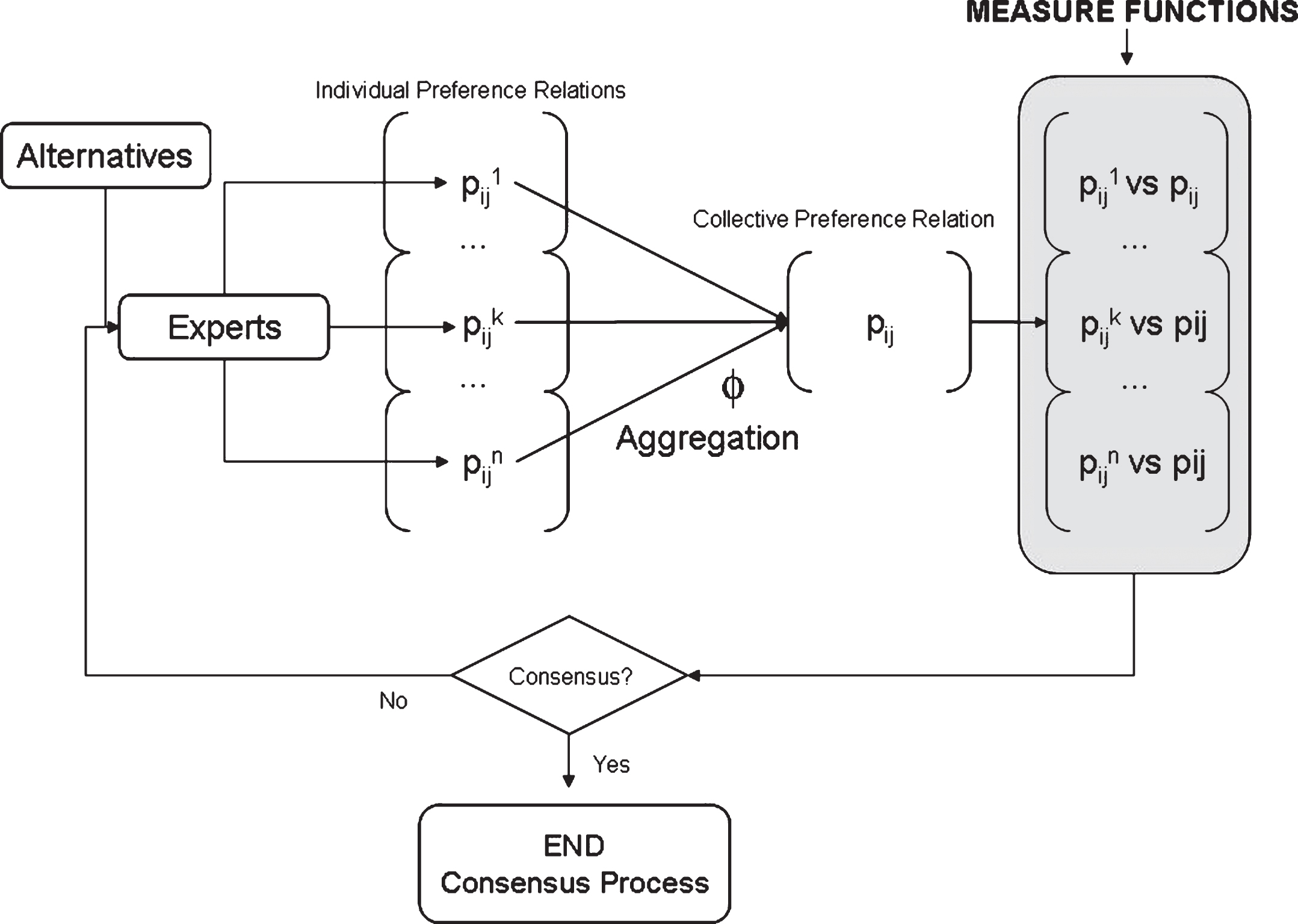
In a consensus process we have to define a coincidence criterion to calculate those consensus measures that allows us to lead to the process of reaching consensus. This is a dynamic process (see Figs.1 and 2) in which a previously agreed consensus value and/or number of rounds serves as control of the process. If any of these values is exceeded, the process ends and, if not, a feedback mechanism provides advice to experts in order to approximate their positions.

Fig.1

Consensus Model based on distance functions.

Fig.2

Consensus Model for C_x method.

Two of the main approaches that can be used in a consensus process are the notion of soft coincidence among preferences and the concept of the coincidence among solutions [4 , 19].

2.3.1 Consensus models based on soft coincidence among preferences

In GDM problems it is very extended to consider consensus as an iterative procedure where, after several rounds of discussion, accord is achieved. Then, it is assumed that the process of reaching consensus is led by two consensus measures [5, 6]: the consensus measure to evaluate the level of consensus in every one of the rounds of discussion and the proximity measure to lead to the discussion stage. Furthermore, these consensus measures allow us to discover information about the consensus state at every level of representation, namely, pairs of alternatives, alternatives and complete relation. In such a way, the degree of agreement among experts is determined by computing the similarity existing between their preferences by means of distance functions [4, 5, 19].

Definition 3. Let Λ be a set of elements, then $d: Λ \times Λ \to ℝ$ is said to be a distance function defined on Λ if it is nonnegative, d (x, y) ≥0, symmetric, d (y, x) = d (x, y) and reflexive, d (x, x) =0, for all x, y ∈ Λ.

Definition 4. $s: Λ \times Λ \to ℝ$ is said to be a similarity function defined on Λ when s is nonnegative, is symmetric, and if it is satisfied: s (x, y) ≤ s (x, x) ∀ x, y ∈ Λ, s (x, y) = s (x, x) ⇔ x = y.

It is very easy to transform a similarity s to a distance d bounded by the unit value, and one possibility could be the following: d = 1 - s [14]. Then, the different consensus degrees utilized to control the consensus phase are deduced by merging the similarity of the values of preference supplied by the experts for every two alternatives. On the other hand, the proximity measures used to generate feedback used in the discussion rounds are determined by evaluating the similarity that there exists between the preferences expressed by every expert inside the group and the preferences in the collective.

This paper is focussed on the consensus degrees that we compute in a consensus process. The consensus degrees are obtained as follows:

Given an expert, r, the similarity between his/her preferences and the corresponding preferences provided by the others experts inside the group is represented in an individual similarity matrix, ${SM}^{r} = ({sm}_{ij}^{r})$ , obtained as: ${sm}_{ij}^{r} = s (p_{ij}^{r}, p_{ij})$ (6) where $p_{ij}^{r} = (p_{ij}^{r}, \dots, p_{ij}^{r})$ , $p_{ij} = (p_{ij}^{1}, \dots, p_{ij}^{r - 1},$ $p_{ij}^{r + 1}, \dots, p_{ij}^{m})$ and s [0, 1] ^m-1 × [0, 1] ^m-1 → [0, 1] is a similarity function. If ${sm}_{ij}^{r}$ =1 then $p_{ij}^{r}$ and p_ij are equal, while if ${sm}_{ij}^{r}$ =0 $p_{ij}^{r}$ and p_ij are totally different.

A consensus matrix, CM = (cm_ij), is defined as $\forall i, j \in {1, \dots, n} : {cm}_{ij} = φ ({sm}_{ij}^{1}, \dots, {sm}_{ij}^{m})$ (7)

being φ the OWA operator introduced in Definition 2.

Consensus degrees are determined in the feasible levels of computation in the following way:

Consensus on the pairs of alternatives: This degree of consensus, called cp_ij, is computed for every two alternatives (x_i, x_j), and it represents the accord among all the experts on the two alternatives: ${cp}_{ij} = {cm}_{ij}$ (8) $\forall i, j = 1, \dots, n, i \neq j .$

Consensus on alternatives, ca_i. It is used to evaluate the accord among all the experts on the alternative x_i. This consensus degree is obtained through the aggregation of the degrees of consensus of all the pairs of alternatives affecting alternative x_i: ${ca}_{i} = φ ({cp}_{ij}, {cp}_{ji}; j = 1, \dots, n, i \neq j)$ (9)

Consensus on the relation, cr. This consensus degree is used to evaluate the global accord among all the experts. This degree of consensus is derived from fusing the degrees of consensus on alternatives: $cr = φ ({ca}_{i}; i = 1, \dots, n)$ (10)

In this study our interest is focused on the consensus degree obtained in the level 3.

In order to support experts to agree a particular solution so that their individual positions converge, a consensus level γ ∈ [0, 1] is set beforehand. The decision-making session ends as the required consensus level is reached, cr ≥ γ, and then, by applying the selection procedure the solution is achieved. In another way, a group discussion session is performed so as to permit the change of preferences to experts. In this discussion session, a feedback mechanism build around both measures of adjacency and a collection of recommendations is applied to aid the experts in modifying their preferences as displayed in Fig. 1.

The rules used to provide advice to experts are based on a comparison between the individual and collective preferences:

DR.1. If $p_{ij}^{i} - p_{ij}^{c} < 0$ , expert e_i will be recommended to increase $p_{ij}^{i}$ and decrease $p_{ji}^{i}$ in the same quantity.

DR.2. If $p_{ij}^{i} - p_{ij}^{c} > 0$ , expert e_i will be recommended to decrease $p_{ij}^{i}$ and increase $p_{ji}^{i}$ in the same quantity.

DR.3. If $p_{ij}^{i} - p_{ij}^{c} = 0$ , expert e_i will not receive a recommendation of change $p_{ij}^{i}$ and $p_{ji}^{i}$ .

More details can be consulted in [20, 31].

As it is pointed out in [12] the consensus reaching process depends on the particular distance function used to calculate the similarity [10 , 56]. As then, in this paper we consider the distance functions that are defined below.

Definition 5. (Manhattan distance) A Manhattan distance d₁ is defined as a function d₁ : Rⁿ × Rⁿ → R $d_{1} (a, b) = \sum_{i = 1}^{n} | a_{i} - b_{i} |$ (11)

Definition 6. (Euclidean distance) An Euclidean distance d₂ is defined as a function d₂ : Rⁿ × Rⁿ → R $d_{2} (a, b) = \sqrt{\sum_{i = 1}^{n} | a_{i} - b_{i} |^{2}}$ (12)

Definition 7. (Cosine distance) A Cosine distance d₃ is defined as a function d₃ : Rⁿ × Rⁿ → R $d_{3} (a, b) = \frac{\sum_{i = 1}^{n} a_{i} \cdot b_{i}}{\sqrt{\sum_{i = 1}^{n} a_{i}^{2}} \cdot \sqrt{\sum_{i = 1}^{n} b_{i}^{2}}}$ (13)

Definition 8. (Dice distance) A Dice distance d₄ is defined as a function d₄ : Rⁿ × Rⁿ → R $d_{4} (a, b) = \frac{2 \cdot \sum_{i = 1}^{n} a_{i} \cdot b_{i}}{\sum_{i = 1}^{n} a_{i}^{2} + \sum_{i = 1}^{n} b_{i}^{2}}$ (14)

Definition 9. (Jaccard distance) A Jaccard distance d₅ is defined as a function d₅ : Rⁿ × Rⁿ → R $d_{5} (a, b) = \frac{\sum_{i = 1}^{n} a_{i} \cdot b_{i}}{\sum_{i = 1}^{n} a_{i}^{2} + \sum_{i = 1}^{n} b_{i}^{2} - \sum_{i = 1}^{n} a_{i} \cdot b_{i}}$ (15)

2.3.2 Consensus model based on coincidence among solutions

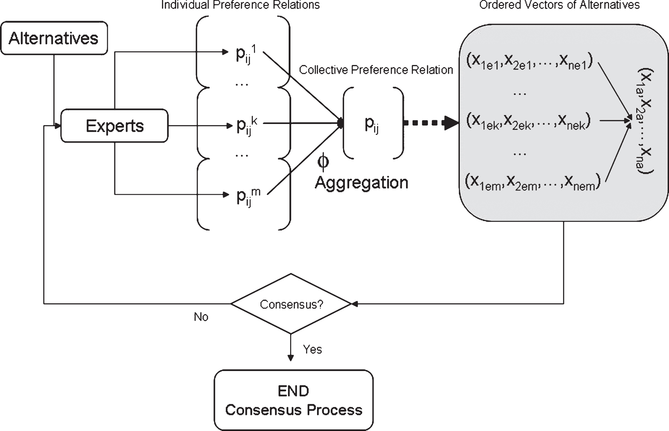
An alternative approach to the aforementioned consensus process consists of measuring consensus by considering the position of the alternatives in each particular solution expresed by the experts [20]. This model takes into account two different criteria: a consensus measure that calculates the accordance among experts so as to conduct the consensus process to the ultimate solution and a proximity measure which calculates the accordance among particular experts’ opinions and the opinion in the group so as to conduct the debate of the group in the process of consensus. Both measures compare solutions, the individual and the collective, instead of the respective preferences as in the model described in subsection 2.3.1. By comparing the position of the alternatives in each solution, this comparison procedure allows to reflect the real consensus situation at each moment of the consensus process. This means that, at each step of the process of consensus, the first thing to do is to apply the selection process to obtain a temporary collective solution, and then measure the closeness of that solution to the individual solution [20].

Let $V^{i} = (V_{1}^{i}, \dots, V_{n}^{i})$ be the individual solution of expert e_i, where $V_{j}^{i}$ is the position of the alternative x_j for the ith expert, and let $V^{c} = (V_{1}^{c}, \dots, V_{n}^{c})$ be the collective solution, where $V_{j}^{c}$ is the position of the alternative x_j in that collective solution. The position of the alternatives in the solution vectors of alternatives is used to calculate both, the consensus measure and the proximity measure instead of the choice degrees associated with the alternatives [55].

The adjacency of each expert for each alternative, p_i (x_j), is calculated by means of the comparison of the position of that alternative in the experts’s particular solutions, {Vⁱ ; i = 1, …, m }, and its position in the collective solution, V^c, through the function [20]: $p_{i} (x_{j}) = {(\frac{| V_{j}^{c} - V_{j}^{i} |}{n - 1})}^{b} \in [0, 1]$ with 0 ≤ b ≤ 1. The parameter b is used to control the rigor of the consensus process; values of b close to one decrease the number of rounds to develop in the process of group discussion, and values of b close to zero increase the number of rounds. Appropriate values for this parameter are: 0.5, 0.7, 0.9, 1 [20]. In this paper, we use b = 1 in order to make the number of rounds small.

The degree of consensus for all experts on each alternative x_j is derived from: $C (x_{j}) = 1 - \sum_{i = 1}^{m} \frac{p_{i} (x_{j})}{m}$ (16)

Finally, the consensus measure over the collection of alternatives is calculated by accumulating the values C (x_j): $C_{x} = (1 - β) \cdot \sum_{i = 1}^{v} \frac{C (x_{i})}{v} + β \cdot \sum_{j = 1}^{w} \frac{C (x_{j})}{w}$ (17) where w denotes the cardinal of X_sol; v denotes the cardinal of X - X_sol; and β ∈ [0, 1]. The parameter β is employed to control the influence of the consensus degree of the solution alternatives over the consensus measure on the set of alternatives. High values of β represent high influence of the consensus degree of the solution alternatives on the global consensus degree. Adequate values for this parameter are: 0.7, 0.8 and 0.9 [20]. In this paper, we use β = 0.9.

The above model is represented in Fig. 2.

When the consensus measure C_x has not reached the required level of consensus, a feedback mechanism indicates the experts to change their opinions in a similar way to the one described in the Section 2.3.1. In this case, the rules used to make experts change their opinions are based on a comparison between individual and collective solutions. This way, for the ith expert, e_i, the opinion is changed using the following rules:

R.1. If $| V_{j}^{c} - V_{j}^{i} | < 0$ , then increase evaluations associated with alternative x_j.

R.2. If $| V_{j}^{c} - V_{j}^{i} | > 0$ , then decrease evaluations associated with alternative x_j.

R.3. If $| V_{j}^{c} - V_{j}^{i} | = 0$ , do not change evaluations associated with alternative x_j.

More details can be consulted in [20].

In this paper we examine whether the use of the aforementioned approaches produces differences which are significant in measuring the consensus and accelerating the convergence of the process of consensus. Following the study carried out in our previous paper [12] we consider the distance functions d_i, i = 1, …, 5, given in Equations (11)–(15) to handle the model based on the soft coincidence among preferences, and the consensus measure C_x given in expression (17) to deal with the model based on the concordance among solutions [20].

3 Experimental design and comparative study

As mentioned before, two approaches can be considered to calculate soft consensus measures: concordance among expert preferences and concordance among individual solutions. In the first approach, the coincidence is obtained by evaluating the similarity among the expert preferences by means of distance functions, and in the second one the concordance is calculated by measuring the similarity among the solutions proposed by these experts using the consensus measure C_x.

Following the guidelines presented in [12], the hypothesis we are testing in this paper can be established as follows: The application of Manhattan, Euclidean, Cosine, Dice and Jaccard distance functions versus the consensus measure C_x in GDM problems do not produce significant differences in the measurement of consensus

To test this hypothesis, we generated ten sets of fuzzy preference relations in a ramdom way for every one of the possible combinations of alternatives: four, six and eight, and experts: four, six, eight, ten and twelve. Moreover, the distinct distance functions, d_i, i = 1, …, 5, given in equations from (11) to (15), and the consensus measure over the collection of alternatives, C_x, given in Equation (17), were successively used to size up consensus at the relation level, employing the OWA operators introduced in Subsection 2.2. We compared every distance function with the consensus measure over the collection of alternatives, d_i vs C_x (i = 1, …, 5), so that we finished handling two related samples.

The problem of two related samples can be adressed from two points of view: parametric and nonparametric. In the parametric case, the t-test is applied provided that the assumption of normality and independence distribution of the difference scores can be assumed [26, 37]. This way, the t-test could be applied to the problem we are dealing with if these hypothesis could be assumed on the population from which the random sample of fuzzy preference relation is selected. But, we have no information that could allow to identify the nature of the population from which the random sample of fuzzy preference relations is selected and we have any knowledge about any of its parameters. Therefore, we conclude that nonparametric test are most appropriate in our experimental study.

For continuous data and two related samples, the main nonparametric tests available are the sign test and the Wilcoxon signed-rank test [12 , 42]. Since the Wilcoxon signed-rank test incorporates more information about the data it is more powerful than the sign test, and so it is preferable to be used in our study.

As a further step, it would be very interesting to be able to discriminate among the distance functions d_i, i = 1, …, 5, given in Equations (11)–(15), and the consensus measure over the collection of alternatives C_x, given in Equation (17). This discrimination procedure can be achieved through the mean ranks used in the nonparametric Friedman test to deal with several related samples [17 , 37]. The ranking that can be achieved when these mean ranks are considered will allow to emphasize the magnitude of the differences between the aforementioned functions for the calculation of the consensus values.

In the following subsections we describe in detail these two statistical techniques to better understand their application in the subsequent study.

3.1 Wilcoxon signed-ranks matched-pairs test

Let X₁, X₂, …, X_n denote a n-size random sample from a distribution function F which is continuous, let p denote a value in $(0, 1) \in ℝ$ , and let ξ_p (F) indicate the p-quantile of F, that is, ξ_p (F) is that value which provides a solution of the equation F (x) = p. When p = 0.5, ξ_0.5 (F) is called median of the distribution function F.

A problem of symmetry and location consists in testing the hypothesis H₀ : ξ_0.5 (F) = ξ₀ and F is symmetric against the hypothesis H₁ : ξ_0.5 (F) ≠ ξ₀ and F is not symmetric. A nonparametric statistical technique known as Wilcoxon signed ranks test supplies a hypothesis test that considers the measure of the differences between the observed values and the quantile in H₀ with the aim of performing a problem of symmetry and location.

Let H₀ : ξ_0.5 (F) = ξ₀ be the null hipothesis and let D_i = X_i - ξ₀, i = 1, 2, …, n, be the differences to the hypothesized value. Under H₀ positive and negative differences are expected to be dispersed, so that the expected number of negative differences will be n/2 and negative and positive differences of equal absolute magnitude should take place with the same probability.

Let |D_i|, i = 1, 2, …, n, be the absolute values of D_i, i = 1, 2, …, n, and let us rank them from 1 (for the smallest) to n (for the largest). If T₊ denotes the sum of ranks assigned to those $D_{i}^{'} s$ that are positive and T_- denotes the sum of ranks assigned to those $D_{i}^{'} s$ that are negative, it follows that $T_{+} +: T_{-} = \sum_{k = 1}^{n} k = \frac{n (n + 1)}{2}$

So, T₊ and T_- are linearly related and provide equivalent rules. A large value of T₊ indicates that most of the larger ranks are assigned to positive $D_{i}^{'} s$ , so that they support H₁ : ξ_0.5 (F) > ξ₀. The same assertion applies to the alternative H₁ : ξ_0.5 (F) < ξ₀ and H₁ : ξ_0.5 (F) ≠ ξ₀.

This way the test rejects H₀ : ξ_0.5 (F) = ξ₀ to accept H₁ : ξ_0.5 (F) > ξ₀ if T₊ > c₁; equivalently, if t₀ denotes the observed value of T₊, it rejects H₀ if p₀ = P_{H
₀} [T₊ ≥ t₀] ≤ α, being α the significance level of the test. The test rejects H₀ to accept H₁ : ξ_0.5 (F) < ξ₀ if T_- > c₂ or p₀ = P_{H
₀} [T_- ≥ t₀] ≤ α, being t₀ the observed value of T_-. And the test rejects H₀ to accept H₁ : ξ_0.5 (F) ≠ ξ₀ if T₊ > c₃ or T_- > c₄ being values c_i the critical region borders, or, equivalently, if p₀ = 2(smaller tail probability).

Under H₀, the common distribution of T₊ and T_- is symmetric about the mean E [T₊] = n (n + 1)/4 with variance var [T₊] = n (n + 1) (2n + 1)/24. For large n, the standardized T₊ has approximately a standard normal distribution.

If the available data are matched-paired, {(X_i, Y_i) , i = 1, …, n}, being derived from applying two treatments to the same set of subjects, to test H₀ : ξ_0.5 (F_{X_i-Y_i}) = ξ₀ against the possible alternatives Wilcoxon’s test is carried out in the same way as in the case of one sample by taking D_i = X_i - Y_i - ξ₀ [12].

3.2 Friedman mean ranks

The analysis of data resulting from k-related samples can be performed using various nonparametric techniques. One of them addresses the problem as an extension of the two-way analysis of variance for a randomized block design when the assumption that distributions are continuous replaces the assumption of normality.

Let (X_i1, …, X_ik), i = 1, …, n, be a random sample from a k-variate continuous type distribution function. The data may be arranged in n rows (blocks) and k columns (treatment/measure). The observations in different rows are independent and those in different columns are dependent. The observation x_ij then corresponds to the ith block and jth treatment/measure, j = 1, …, k and i = 1, …, n.

In order to test the hypothesis that measure effects are all equal against the hypothesis that measure effects are not all equal, the Friedman procedure [37] involves replacing each observation in a block by its rank. The rank of the jth observation in the ith block, R (x_ij) = R_ij, is the value from 1 to k obtained by consecutively numbering the observations X_ij, j = 1, …, k. So, for each block, the observed values are sorted for each measure and ranked from 1 (the lowest value in the block) up to k (the highest value of the block). Hence ranks are assigned separately for each block.

Let R_j denotes the sum of ranks for jth measure, j = 1, …, k, $R_{j} = \sum_{i = 1}^{n} R_{ij}$ . The mean rank for the jth measure, j = 1, …, k, is defined as ${\bar{R}}_{j} = \frac{R_{j}}{n}$

4 Experimental analysis

In order to develop our study we configure a set of ten GDM problems randomly elaborated for every feasible mixtures of expert numbers: four, six, eight, ten and twelve, and alternatives: four, six and eight. Three executions were done for each one of these GDM problems. In each execution we use one of the three distinct OWA operators aforementioned to calculate the consensus degree. In what follows, we summarize the results obtained by applying the results mentioned above, the Wilcoxon statistical test and the Friedman mean ranks.

4.1 Statistical test results

Table 1 shows the p-value for each one of the distances used in our experimental study versus C_x. To better understand this table and the following ones, from now on, d₁ is denoted by “Ma”, d₂ by “Eu”, d₃ by “Co”, d₄ by “Di” and, finally, d₅ is denoted by “Ja”. In view of the results, it follows that the hypothesis tested and displayed in Section 3 is rejected.

Table 1
Wilcoxon signed-ranks matched-pairs statistical test results

Comparison Ma - C_x Eu - C_x Co - C_x Di - C_x Ja - C_x

Sig. (2-tailed) ,000 ,000 ,000 ,000 ,013

Comparison	Ma - C_x	Eu - C_x	Co - C_x	Di - C_x	Ja - C_x
Sig. (2-tailed)	,000	,000	,000	,000	,013

The comparison between different distance functions and C_x to measure consensus produces significantly different results in all possible combinations used in the experiment. In particular, we observe a p-value less or equal than 0, 05 (predetermined significance level α) in all cases. In fact, in four of the cases the p-value is lower than 0, 001 (α), except for the Jaccard distance function, where the p-value is 0,013.

We note that, at the relation level, measurement of consensus is affected significantly by the use of a different distance function in comparison with C_x. Results differ significantly depending on the distance function to be compared. Obviously, the comparison of different distance functions, for which significant variation has been established, could affect the convergence of the consensus process at this level.

Moreover, it can be observed that the results of the C_x consensus measure and the Jaccard distance function are similar. This fact leads us to think that the consensus measure C_x can be used as an alternative to the Jaccard distance function in the considered situation, and also that a consensus model based on the coincidence among solutions could replace a model based on the among experts preferences and vice versa in the calculation of the degree of consensus when dealing with a situation like this one.

4.2 Friedman mean ranks results

Let us now analyze the results derived from Friedman mean ranks according to quantifiers, experts and alternatives.

Table 2 shows mean ranks of all methods according to the linguistic quantifiers considered in this study: “at least half”, “most of” and “as many as possible”. As regards to the first linguistic quantifier, we observe that the Jaccard distance function is closer to C_x than the rest of distance functions. In this case the Jaccard distance function achieves bigger values than C_x. We also note that as for the linguistic quantifier “most of”, C_x is positioned between the Jaccard and Dice distance functions. In this situation the Jaccard distance function is nearer to C_x than the Dice distance function. Regarding to the linguistic quantifier “as many as possible”, it can be seen that C_x is positioned between the Jaccard and Dice distance functions as in the previous situation but, in this case, C_x is nearer to the Dice distance function.

Table 2
Mean ranks according to quantifiers

“at least half” “most of” “as many as possible”

Method Mean rank Method Mean rank Method Mean rank

C _x 1,21 Ja 1,33 Ja 1,04

Ja 2,53 C _x 2,25 C _x 2,81

Ma 3,47 Di 3,53 Di 3,06

Di 4,21 Eu 4,31 Co 4,07

Eu 4,35 Co 4,53 Eu 4,57

Co 5,23 Ma 5,06 Ma 5,45

“at least half”	“most of”	“as many as possible”
C _x	1,21	Ja	1,33	Ja	1,04
Ja	2,53	C _x	2,25	C _x	2,81
Ma	3,47	Di	3,53	Di	3,06
Di	4,21	Eu	4,31	Co	4,07
Eu	4,35	Co	4,53	Eu	4,57
Co	5,23	Ma	5,06	Ma	5,45

Table 3 shows mean ranks for different methods and different number of experts considered in this study. In this case C_x is situated between the Jaccard and Dice distance functions except for the 4 experts case where the results are different from the ones obtained from 6 experts. We also note that, in all cases except the above-mentioned 4 experts case, C_x gets values closer to the Jaccard distance function than the Dice distance function.

Table 3

Mean ranks according to experts

4 experts		6 experts		8 experts		10 experts		12 experts
Method	Mean rank	Method	Mean rank	Method	Mean rank	Method	Mean rank	Method	Mean rank
Ja	2,32	Ja	1,59	Ja	1,48	Ja	1,38	Ja	1,39
Eu	2,39	C _x	1,97	C _x	1,70	C _x	1,71	C _x	1,77
Ma	2,57	Di	3,80	Di	3,39	Di	3,13	Di	2,98
C _x	3,31	Eu	4,30	Co	4,40	Co	4,13	Co	4,00
Di	4,70	Ma	4,54	Eu	4,88	Eu	5,19	Eu	5,28
Co	5,71	Co	4,80	Ma	5,16	Ma	5,46	Ma	5,59

On the other hand Table 4 shows mean ranks of different methods for the three possible number of alternatives proposed in the study. We observe that the behavior of C_x is very stable in all cases. It can be pointed out that the values of C_x are situated between the ones of the Jaccard and Dice distance functions.

Table 4

Mean ranks according to alternatives

4 alternatives		6 alternatives		8 alternatives
Method	Mean rank	Method	Mean rank	Method	Mean rank
Ja	1,70	Ja	1,59	Ja	1,60
C _x	2,20	C _x	1,97	C _x	1,95
Di	3,63	Di	3,80	Di	3,57
Eu	4,27	Eu	4,30	Eu	4,53
Ma	4,56	Co	4,54	Co	4,58
Co	4,65	Ma	4,80	Ma	4,77

Table 5 shows mean ranks for all methods and samples. It can be observed that the Jaccard and Dice distance functions are closer to C_x in their mean rank positions than the rest of functions, being Jaccard the closest one.

Table 5

Global mean rank

Method	Mean rank
Ja	1,63
C _x	2,09
Di	3,60
Eu	4,41
Co	4,61
Ma	4,66

In summary, we perceive that at the level of relation the evaluation of consensus depend on the distance functions which are used instead of C_x. Therefore, the utilization of distinct distance functions could influence the convergence of the consensus reaching process at the level of relation. Furthermore, the results obtained suggest that the Jaccard distance function is the best option versus C_x method, and the second option should be the Dice distance function.

The experimental study performed in this paper allows us to visualize a ranking of the different distance functions useful for their application as it is illustrated in Fig. 3. Most of metrics reach a consensus speed faster than C_x, so if we want a faster convergence to consensus we would measure consensus on preferences with Manhattan, Cosine or Euclidian metric.

Fig.3

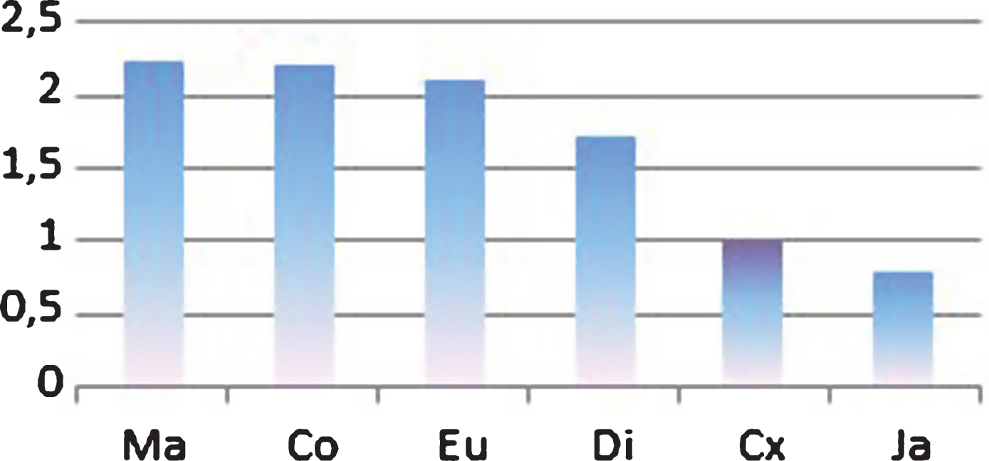
Global consensus speed.

If required in a consensus process, the values of C_x model on the set of solutions could be substituted for those provided by the the appropriate distance function on the alternatives.

These results are coherent with the ones obtained in [12] but in this paper we also obtain a quantitative classification for the considered methods.

Finally, note that the values obtained for the consensus measure C_x are placed between the values obtained for the Dice and Jaccard distance functions. This way, it seems to be confirmed that C_x can be considered a different measure but comparable with the measures already analyzed [12], being the values of C_x closer to those of the Jaccard distance functuion and being able to replace or be replaced by them.

5 Example

As an application of the study carried out let us consider the example introduced in our previous paper [12]. A GDM problem with four alternatives and four experts is performed using the OWA operator guided by the linguistic quantifier “as many as possible” and a consensus threshold γ = 0.75. It is assumed that the initial set of individual fuzzy preference relations are the same as the ones that appear in Example in [12]. $\begin{matrix} (\begin{matrix} 0.50 & 0.11 & 0.23 & 0.32 \\ 0.89 & 0.50 & 0.44 & 0.12 \\ 0.77 & 0.66 & 0.50 & 0.21 \\ 0.68 & 0.88 & 0.79 & 0.50 \end{matrix}) (\begin{matrix} 0.50 & 0.65 & 0.91 & 0.70 \\ 0.35 & 0.50 & 0.82 & 0.63 \\ 0.09 & 0.18 & 0.50 & 0.34 \\ 0.30 & 0.37 & 0.66 & 0.50 \end{matrix}) \\ (\begin{matrix} 0.50 & 0.43 & 0.81 & 0.64 \\ 0.57 & 0.50 & 0.72 & 0.91 \\ 0.19 & 0.28 & 0.50 & 0.43 \\ 0.36 & 0.09 & 0.57 & 0.50 \end{matrix}) (\begin{matrix} 0.50 & 0.32 & 0.41 & 0.63 \\ 0.68 & 0.50 & 0.62 & 0.93 \\ 0.59 & 0.38 & 0.50 & 0.81 \\ 0.37 & 0.07 & 0.19 & 0.50 \end{matrix}) \end{matrix}$

5.1 First round

At the relation level, the Jaccard distance function provides a consensus degree of 0.43, C_x of 0.49 and the Cosine distance function of 0.66. The global consensus degree is lower than the threshold consensus level, so that experts receive feedback to modify their preference relations.

5.2 Second round

The new fuzzy preference relations are the same that appear in [12]. Using the Cosine distance function the consensus degree results in 0.81 which is greater than the threshold consensus level and the consensus process ends. However, if the Jaccard distance function or C_x are used, it would be necessary to continue with the consensus reaching process since the consensus degree levels are 0.53 and 0.61 respectively.

5.3 Third round

The new fuzzy preference relations are the ones that appear in [12]. The Jaccard distance function results in a consensus degree level of 0.60 and C_x of 0.65.

5.4 Fourth round

The new fuzzy preference relations appear in [12]. Using C_x we would have had a consensus degree level of 0.79 which is greater than the threshold consensus level and the consensus process ends. However, using again the Jaccard distance function we need to continue with the consensus reaching process since the consensus degree level would be 0.69.

5.5 Fifth round

The new fuzzy preference relations areappear in [12]. The Jaccard distance function results in a consensus degree level of 0.78, the consensus reaching process stops and the selection process is activated to derive the solution of consensus.

6 Conclusion

We have analyzed the behaviour of two widely used consensus models based on two types of coincidence in GDM problems with fuzzy preference relations. In the first case the coincidence is obtained through similarity measured among expert preferences by using several distance functions. We have considered five distance functions commonly used in measuring experts’ preferences: Manhattan, Euclidean, Cosine, Dice and Jaccard. In the second case, the coincidence is derived from similarity calculated through the individual solutions provided by expert preferences. We have used the consensus measure C_x on the set of solution of alternatives. We have presented a comparative experiental study based on the utilization of Friedman mean ranks and the nonparametric Wilcoxon’s test. The results are interesting since our experimental study has shown that the consensus model based on the use of distance functions compared with the model based on consensus measure C_x produce significantly different results in most of the GDM problems performed. However, the similarity between the results of the C_x consensus measure and the Jaccard distance function unveils two relevant elements. On the one hand, a consensus model based on the coincidence among solutions can replace a model based on coincidence among expert preferences and vice versa in the calculation of the degree of consensus when dealing with a situation such as the one contemplated in this paper. On the other hand, the consensus measure C_x can be used as an alternative to the Jaccard distance function in the considered situation. The analysis of the results allows to draw a ranking of the different measures used according to the degree of consensus. In addition, this classification can be successfully used to control the speed of convergence of the consensus process.

Footnotes

Acknowledgments

The authors would like to acknowledge the FEDER financial support from the project TIN2016-75850-R.

References

Bordogna

, Fedrizzi

and Pasi

, A linguistic modeling of consensus in group decision making based on OWA operators, IEEE Transactions on Systems Man and Cybernetics-Part A: Systems and Humans 27(1) (1997), 126–133.

Cabrerizo

F.J.

, Al-Hmouz

, Morfeq

, Balamash

A.S.

, Martinez

M.A.

and Herrera-Viedma

, Soft consensus measures in group decision making using unbalanced fuzzy linguistic information, Soft Computing 21(11) (2017), 3037–3050.

Cabrerizo

F.J.

, Herrera-Viedma

and Pedrycz

, A method based on PSO and granular computing of linguistic information to solve group decision making problems defined in heterogeneous contexts, European Journal of Operational Research 230(3) (2013), 624–633.

Cabrerizo

F.J.

, Moreno

J.M.

, Pérez

I.J.

and Herrera-Viedma

, Analyzing consensus approaches in fuzzy group decision making: Advantages and drawbacks, Soft Computing 14(5) (2010), 451–463.

Cabrerizo

F.J.

, Chiclana

, Al-Hmouz

, Morfeq

, Balamash

A.S.

and Herrera-Viedma

, Fuzzy decision making and consensus: Challenges, Journal of Intelligent & Fuzzy Systems 29(3) (2015), 1109–1118.

Cabrerizo

F.J.

, Pérez

I.J.

and Herrera-Viedma

, Managing the consensus in group decision making in an unbalanced fuzzy linguistic context with incomplete information, Knowledge-Based Systems 23(2) (2010), 169–181.

Cabrerizo

F.J.

, Ureña

M.R.

, Pedrycz

and Herrera-Viedma

, Building consensus in group decision making with an allocation of information granularity, Fuzzy Sets and Systems 255 (2014), 115–127.

Capuano

, Chiclana

, Fujita

, Herrera-Viedma

and Loia

, Fuzzy group decision making with incomplete information guided by social influence, IEEE Transactions on Fuzzy Systems (2017). doi 10.1109/TFUZZ.2017.2744605

Carlsson

, Ehrenberg

, Eklund

, Fedrizzi

, Gustafsson

, Lindholm

, Merkuryeva

, Riissanen

and Ventre

A.G.S.

, Consensus in distributed soft environments, European Journal of Operational Research 61(1-2) (1992), 165–185.

10.

Cha

S.H.

, Comprehensive survey on distance/similarity measures between probability density functions, International Journal of Mathematical Models and Methods in Applied Sciences 4(1) (2007), 300–3007.

11.

Chen

S.M.

, Yeh

M.S.

and Hsiao

P.Y.

, A comparison of similarity measures of fuzzy values, Fuzzy Sets and Systems 72(1) (1995), 79–89.

12.

Chiclana

, Tapia

J.M.

and Del

M.J.

, Moral and E. Herrera-Viedma, A statistical comparative study of different similarity measures of consensus in group decission making, Information Sciences 221 (2013), 110–123.

13.

del

M.J.

, Chiclana

Moral, F.

, Tapia

J.M.

and Herrera-Viedma

. A comparative study on consensus measures in group decision making, Int J of Intelligent Systems (2018). In press, https://doi.org/10.1002/int.21954

14.

Deza

M.M.

, Deza

Elena

, Encyclopedia of Distances2009, Springer Heidelberg, Berlin.

15.

Dong

and Herrera-Viedma

, Consistency-driven automatic methodology to set interval numerical scales of 2-tuple linguistic term sets and its use in the linguistic GDM with preference relation, IEEE Transactions on Cybernetics 45(4) (2015), 780–792.

16.

Dong

, Zhang

and Herrera-Viedma

, Integrating experts’ weights generated dynamically into the consensus reaching process and its applications in managing non-cooperative behaviors, Decision Support Systems 84 (2016), 1–15.

17.

Friedman

, The use of ranks to avoid the assumption of normality implicit in the analysis of variance, Journal of the American Statistical Association American Statistical Association 32(200) (1937), 675–701.

18.

Herrera-Viedma

, Cabrerizo

F.J.

, Chiclana

, Wu

, Cobo

M.J.

and Samuylov

, Consensus in group decision making and social networks, Studies in Informatics and Control 26(3) (2017), 259–268.

19.

Herrera-Viedma

, Cabrerizo

F.J.

, Kacprzyk

and Pedrycz

, A review of soft consensus models in a fuzzy environment, Information Fusion 17 (2014), 4–13.

20.

Herrera-Viedma

, Herrera

and Chiclana

, A consensus model for multiperson decision making with different preference structures, IEEE Transactions on Systems, Man and Cybernetics, Part A: Systems and Humans 32(3) (2002), 394–402.

21.

Kacprzyk

and Fedrizzi

, Soft consensus measures for monitoring real consensus reaching processes under fuzzy preferences, Control and Cybernetics 15 (1986), 309–323.

22.

Kacprzyk

and Fedrizzi

, A soft measure of consensus in the setting of partial (fuzzy) preferences, European Journal of Operational Research 34(3) (1988), 316–325.

23.

Kacprzyk

, Fedrizzi

and Nurmi

, Group decision making and consensus under fuzzy preferences and fuzzy majority, Fuzzy Sets and Systems 49(1) (1992), 21–31.

24.

Kacprzyk

, Nurmi

and Fedrizzi

, Consensus under fuzziness 1997 volume 10, Kluwer Publishers Academic.

25.

Lehmann

E.L.

, Nonparametrics: Statistical Methods Based on Ranks, 1975, Holden-Day, San Francisco.

26.

Lehmann

E.L.

and Romano

J.P.

, Testing Statistical Hipothesis, 3, Springer, New York, 2005.

27.

Liao

, Xu

, Zeng

X.J.

and Merigó

J.M.

, Framework of group decision making with intuitionistic fuzzy preference information, IEEE Transactions on Fuzzy Systems 23(4) (2015), 1211–1227.

28.

Liao

, Li

, Zeng

X.J.

and Liu

, A comparison of distinctconsensus measures for group decision making with intuitionistic fuzzy preference relations, International Journal of Computational Intelligence Systems 10 (2017), 456–469.

29.

Liao

, Xu

, Zeng

X.J.

and Xu

D.L.

, An enhanced consensus reaching process in group decision making with intuitionistic fuzzy preference relations, Information Sciences 329 (2016), 274–286.

30.

Liu

, Dong

, Chiclana

, Cabrerizo

F.J.

and Herrera-Viedma

, Group decision-making based on heterogeneous preference relations with self-confidence, Fuzzy Optimization and Decision Making 16(4) (2017), 429–447.

31.

Mata

, Martínez

and Herrera-Viedma

, An adaptive consensus support model for group decision-making problems in a multigranular fuzzy linguistic context, IEEE Transactions on Fuzzy Systems 17(2) (2009), 279–290.

32.

Orlovsky

S.A.

, Decision-making with a fuzzy preference relation, Fuzzy Sets and Systems 1(3) (1978), 155–167.

33.

Palomares

, Martinez

and Herrera

, A consensus model to detect and manage noncooperative behaviors in large-scale group decision making, IEEE Transactions on Fuzzy Systems 22(3) (2014), 516–530.

34.

Pérez

I.J.

, Cabrerizo

F.J.

, Alonso

and Herrera-Viedma

, A new consensus model for group decision making problems with non homogeneous experts, IEEE Transactions on Systems, Man and Cybernetics: Systems 44(4) (2014), 494–498.

35.

Pérez

I.J.

, Cabrerizo

F.J.

and Herrera-Viedma

, A mobile decision support system for dynamic group decision-making problems, IEEE Transactions on Systems, Man and Cybernetics, Part A: Systems and Humans 40(6) (2010), 1244–1256.

36.

Pérez

L.G.

, Mata

, Chiclana

, Kou

and Herrera-Viedma

, Modelling influence in group decision making, Soft Computing 20(4) (2016), 1653–1665.

37.

Rohatgi

V.K.

, Statistical Inference, Publications Inc Dover, 2003.

38.

Roubens

, Fuzzy sets and decision analysis, Fuzzy Sets and Systems 90(2) (1997), 199–206.

39.

Sun

B.Z.

and Ma

W.M.

, An approach to consensus measurement of linguistic preference relations in multi-attribute group decision making and application, Omega 51 (2015), 83–92.

40.

Switalski

, General transitivity conditions for fuzzy reciprocal preference matrices, Fuzzy Sets and Systems 137(1) (2003), 85–100.

41.

Wang

and De

, Baets and E. Kerre, A comparative study of similarity measures, Fuzzy Sets and systems 73(2) (1995), 259–268.

42.

Wilcoxon

, Individual comparisons by ranking methods, Biometrics Bulletin 1(6) (1945), 80–83.

43.

and Chiclana

, A social network analysis trustconsensus based approach to group decision-making problems with interval-valued fuzzy reciprocal preference relations, Knowledge-Based Systems 59 (2014), 97–107.

44.

and Chiclana

, and, E. Herrera-Viedma, Trust based consensus model for social network in an incomplete linguistic information context, Applied Soft Computing 35 (2015), 827–839.

45.

and Xu

, A consistency and consensus based decision support model for group decision making with multiplicative preference relations, Decision Support Systems 52(3) (2012), 757–767.

46.

and Xu

, Possibility distribution based approach for MAGDM with hesitant fuzzy linguistic information, IEEE Transactions on Cybernetics 46(3) (2016), 694–705.

47.

and Xu

, Managing consistency and consensus in group decision making with hesitant fuzzy linguistic preference relations, Omega 65 (2016), 28–40.

48.

and Xu

, A consensus model for large-scale group decision making with hesitant fuzzy information and changeable clusters, Information Fusion 41 (2018), 217–231.

49.

and Cai

, Group consensus algorithms based on preference relations, Information Sciences 181(1) (2011), 150–162.

50.

and Liao

, A survey of approaches to decision making with intuitionistic fuzzy preference relations, Knowledge-Based Systems 80 (2015), 131–142.

51.

Yager

R.R.

, On ordered weighted averaging aggregation operators in multicriteria decision making, IEEE Transactions on Systems, Man and Cybernetics 18(1) (1988), 183–190.

52.

Yager

R.R.

, Quantifier guided aggregation using owa operators, International Journal of Intelligent Systems 11(1) (1996), 49–73.

53.

Yejun

, Jing

and Huimin

, Consensus models based on distance for interval fuzzy and multiplicative preference relations, Journal of Intelligent & Fuzzy Systems 31(1) (2016), 503–518.

54.

Zhang

, Dong

and Herrera-Viedma

, Consensus building for the heterogeneous large-scale GDM with the individual concerns and satisfactions, IEEE Trans On Fuzzy Systems (2017). doi:10.1109/TFUZZ.2017.2697403

55.

Zadrozny

, Consensus Under Fuzziness, An approach to the consensus reaching support in fuzzy environment 1997–Kluwer Academic Publishers.

56.

Zeng

, Some intuitionistic fuzzy weighted distance measures and their application to group decision making, Group Decision and Negotiation 22(2) (2013), 281–298.

An analysis of consensus approaches based on different concepts of coincidence

Abstract

Keywords

1 Introduction

2 Preliminaries

2.1 GDM problem framework

2.2 Selection process

3.1 Wilcoxon signed-ranks matched-pairs test

3.2 Friedman mean ranks

4 Experimental analysis

4.1 Statistical test results

Table 1 Wilcoxon signed-ranks matched-pairs statistical test results Comparison Ma - C x Eu - C x Co - C x Di - C x Ja - C x Sig. (2-tailed) ,000 ,000 ,000 ,000 ,013

5.1 First round

5.2 Second round

5.3 Third round

5.4 Fourth round

5.5 Fifth round

6 Conclusion

Footnotes

Acknowledgments

References

Table 1
Wilcoxon signed-ranks matched-pairs statistical test results

Comparison Ma - C_x Eu - C_x Co - C_x Di - C_x Ja - C_x

Sig. (2-tailed) ,000 ,000 ,000 ,000 ,013