Predictive analysis of impact hazard level of coal rock mass based on fuzzy inference network

Abstract

In view of identification of strong mine quake and rock burst, the mine geology, structural mechanics, mining production data and acoustic emission monitoring process data are infused to build two fuzzy process neural network models based on fuzzy set theory. The model integrates fuzzy logic inference mechanism with process neural network process signal analysis and learning capacity. It presents domain knowledge based on fuzzy set and membership function, and adaptively establishes computational logic and fuzzy decision rules based on process signal distribution features, which can effectively infuse multi-source information and prior knowledge, demonstrating good ability to comprehensively analyze various quantitative and qualitative mixed information and identify microquake features, as well as small sample modeling capacity. It has good adaptability for predictive analysis of strong mine quake and rock burst with uncertainty.

Keywords

Coal rock mass impact fuzzy neural network

1 Introduction

The incidence of coal mine dynamic disaster accidents is closely related to the internal rupture of coal rock mass, that is, stress change. Microquake signal is the precursor information of coal rock mass rupture, but due to the diversity, sudden transiency, uncertainty, easy susceptibility of the signal itself, there are some limitations in microquake monitoring technology applied in coal mines. The impact risk of rock burst is a result of multiple factors such as rock geostress, coal seam characteristics and essential properties of rock mass, which varies with time and space based on geological conditions of mining. There are many influencing factors in the incidence of rock burst, and complex relationship exists between risk prediction and the influencing factors, showing great fuzziness. Meanwhile, prediction parameters themselves are also fuzzy.

According to different monitoring objects and monitoring areas of microseismic and geophone systems, Xia Y. (2011) established a joint evaluation model of impact risk based on microseismic and geophone monitoring in Qianqiu Coal Mine, which improved the rock burst prediction level [1]. In practical engineering and scientific research, the object of information processing for many nonlinear dynamic systems is often the combination of time-varying numerical signals and information with procedural fuzzy rules [2]. Based on this, Qin Zhongcheng (2019) proposed a rock burst coupling evaluation- SPA-ITFN coupling model based on set pair analysis-interval triangular fuzzy number, which led to more precise definition of evaluation levels [3]. Based on the catastrophe progression method combining catastrophe theory and fuzzy mathematics, Jin P. (2013) proposed a new index for the evaluation of rock burstrisk [4]. Zhu F. (2017) proposed an “AHP+entropy weight” combined weighting method for the problem that it is difficult to determine the index weight in the rock burst disaster assessment system model [5]. Based on the acoustic emission mechanism of material stress process, X.W. Li (2013) established a gray cusp catastrophe model of acoustic emission parameters on the basis of grey theory and catastrophe theory [6]. J.W.Shi (2018) used grey correlation (GRA) and set pair analysis (SPA) theory to quantify the risk of rock burst, and constructed an entropy weight (EW) multi-attribute decision-making model based on GRA-SPA. The multi-objective multi-attribute risk assessment of coal mine rock burst was made from two aspects of risk and susceptibility [7]. T.X. Wen (2017) identifies the key factors affecting the risk of ground pressure by using the attribute reduction algorithm of Neighborhood Rough Set (NRS), and then optimizes the penalty factors of selecting support vector machine (SVM) model by combining adaptive Chaos Particle Swarm Optimization (ACPSO), Sub-C and kernel function parameter. The variable reduced by NRS attributes is used as input of ACPSO-SVM model, and then the prediction model of rock burst risk based on NRS-ACPSO-SVM is established [8]. In order to accurately predict the risk of rock burst, T.X. Wen (2017) proposed a prediction model based on Least Square Support Vector Machine (LSSVM) for dynamic integration of optimized Bagging algorithm [9]. Wang J. (2017) proposed a grading evaluation model of rock burst risk based on PCA (primary component analysis) and DDA (distance discriminant analysis) [10].

The incidence of mine quake is subject to coupling control of multiple factors. With the aid of some microquake detection methods, like acoustic monitoring waveforms and energy signals, geostress monitoring data as well as bracket pressure signals, etc., this paper studies the influence of mine quake distribution on rock burst under different conditions. Combining the site situation, it analyzes the mechanism and distribution of the incidence from multiple perspectives of mining speed stability and key layer motion, and then establishes the relationship between microquake and rock burst based on model analysis and knowledge representation.

2 Methods

2.1 Classification and identification of coal rock mass impact hazard based on normalized fuzzy neural network

The normalized fuzzy neural network (NFNN) belongs to a form of fuzzy neural network, which consists of five layers, namely, input layer, fuzzy layer, rule layer, normalization layer and anti-fuzzy output layer. Its characteristic is that under definite number of fuzzy layer membership functions and input output modes, the node number of normalization layer, rule layer and fuzzy layer can be calculated and determined. The network training modifies the connection weight between fuzzy center, rule layer, variance and anti-fuzzy output layer.

The prediction of rock burst intensity based on the infusion of mine geology, structural mechanics, mining production data and acoustic emission monitoring process data is a prominent problem in coal mining, especially in deep mining. Complex geological structure and mining conditions of coal rock mass show many fuzziness in signal acquisition. Under the combination of various fuzzy conditions, there are four degrees of rock burst: strong, medium, weak and noun. To apply normal fuzzy neural network in prediction of rock burst intensity, it is possible to extract the mapping relationship between various types of signals and rock burst intensity, thus realizing intelligent processing of rock burst prediction.

2.1.1 Fuzzy process inference rules

Suppose there are K fuzzy process rules in the domain; If x₁ (t) is A_{k
₁},x₂ (t) is A_{k
₂},⋯,x_n (t) is A_{k
_n},then;y₁ is B_{k
₁},y₂ is B_{k
₂},⋯,y_m is B_{k
_m}; ory₁ = b_{k
₁},y₂ = b_{k
₂},⋯,y_m = b_{k
_m}. In the formula, A_{k
_i} and B_{k
_j} are respectively fuzzy sets on the domain U_i (t) (time-varying signal set) and V_j(tag set). Where,

$X (t) = (x_{1} (t), x_{2} (t), \dots, x_{n} (t))^{T} \in U_{1} (t) \times U_{2} (t) \times \dots \times U_{n} (t)$

and Y = (y₁, y₂, ⋯ , y_m) ^T ∈ V₁ × V₂ × ⋯ × V_m are respectively inputs and outputs of the fuzzy logic system.

Let μ_{A
_ki} be membership function (degree of membership to the fuzzy set A_ki) of k-th node of the input variable x_i (t), and assume that x_i (t) has n_i item nodes for fuzzy partition. That is, the number of fuzzy membership functions corresponding to the input variable x_i (t) is n_i.

2.1.2 Fuzzy normalized process neural network structure

Suppose x_i (t) has n_i item nodes for fuzzy partition, that is, the number of fuzzy membership functions corresponding to the input variable x_i (t) is n_i. Use μ_{A
_ki} to indicate membership function of k-th node of input variable, x_i (t), then the structure of the normalized fuzzy neural network is shown in Fig. 1.

Fig. 1

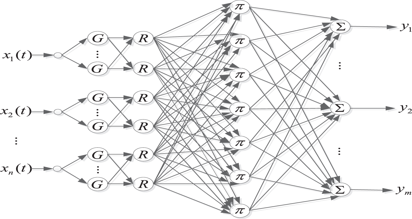
NFPNN structure.

In NFPNN, the first layer is the input layer. This layer has a total of n input nodes, and the input can be a time-varying process signal or fuzzy process information.

The second layer is the fuzzy layer. This layer uses a Gaussian function as a membership function, the output of x_i (t) in the first layer and the j-th node corresponding to the layer is: $μ_{A_{ij}} (x_{i} (t)) = exp (- \frac{| | x_{i} (t) - m_{ij} (t) | |}{σ_{ij}^{2}})$ (1)

Where, m_ij (t) and $σ_{ij}^{2}$ are the typical model sample function and the mean square error, respectively. For instance,m_ij (t) may be a clustering center function obtained by fuzzy aggregation of each mode subclass in the training set; $σ_{ij}^{2}$ is mean square error of the time-varying signal function.

This layer has a total of $N = \sum_{i = 1}^{n} n_{i}$ nodes.

The third layer is a normalized layer which normalizes the output of the second layer, i.e. $μ_{A_{ij}}^{'} (x_{i} (t)) = \frac{μ_{A_{ij}} (x_{i} (t))}{\sum_{j = 1}^{n_{i}} μ_{A_{ij}} (x_{i} (t))}$ (2)

In the formula, $μ_{A_{ij}}^{'} (x_{i} (t))$ indicates normalized output ofμ_{A
_ij} (x_i (t)). The number of nodes in this layer is consistent with that of the second layer, that is, N nodes.

The fourth layer is the rule layer. This layer connects the antecedent (normalized node) with the conclusion node (output node). The connection follows a rule that each rule node is only connected to a normalized node from each of the input components after fuzzification. Please refer to the connection between Layer 3 and Layer 4 in Fig. 1. Therefore, initialization structure of NFPNN network has $K = \prod_{i = 1}^{n} n_{i}$ rule nodes. The output of k-th rule node is:

$z_{k} = \prod_{s \in Ω_{k}} μ_{A_{sk}}^{'} (x_{i} (t)) \prod_{i = 1}^{n} μ_{A_{ik}}^{'} (x_{i} (t))$ (3)

Where, Ω_k is the set of number of layer 3 nodes connected to k-th rule nodes.

The fifth layer is the defuzzification layer. All layer 4 rule nodes are connected to output nodes of this layer. This layer is responsible for the central average defuzzification operation. Suppose this layer has P nodes, then the j– th output component is $y_{l} = \sum_{k = 1}^{K} b_{kj} z_{k}$ (4)

2.1.3 FPNN learning algorithm

For the FPNN model shown in Fig. 3, the connection weight function involving the input layer and the hidden layer is determined by the clustering center of various training sample functions. The parameters demanding adjustment are the weight v_k from the model layer to the output layer as well as FPN hidden layer property parameters a_j, c_j. The error function is defined as

$E = \frac{1}{2} \sum_{s = 1}^{M} \sum_{k = 1}^{K} (d_{sk} - y_{sk})^{2}$ (5)

Using gradient descent algorithm,v_jk and a_j, c_j adjustment amounts are calculated as $- \frac{\partial E}{\partial v_{jk}} = \sum_{s = 1}^{M} (d_{sk} - y_{sk})$ (6)

$\begin{matrix} - \frac{\partial E}{\partial a_{j}} & = & - 2 \sum_{s = 1}^{M} \sum_{k = 1}^{m} (d_{sk} - y_{sk}) v_{jk} h_{j} \\ \frac{1}{s_{j}^{3} (1 + exp (- a_{s} (\int_{0}^{T} \sum_{i = 1}^{n} w_{is} (t) x_{i} (t) dt - c_{s})))} \end{matrix}$ (7)

$\begin{matrix} - \frac{\partial E}{\partial c_{j}} & = & - 2 \sum_{s = 1}^{M} \sum_{k = 1}^{m} (d_{sk} - y_{sk}) v_{jk} h_{j} \\ \frac{1}{s_{j}^{3} (1 + exp (- a_{s} (\int_{0}^{T} \sum_{i = 1}^{n} w_{is} (t) x_{i} (t) dt - c_{s})))} \end{matrix}$ (8)

v_jk and a_j, c_j adjustment amounts are calculated as: $v_{jk} = v_{jk} - α \frac{\partial E}{\partial v_{jk}}$ (9) $a_{j} = a_{j} - β \frac{\partial E}{\partial a_{j}}$ (10) $c_{j} = c_{j} - γ \frac{\partial E}{\partial c_{j}}$ (11)

Where, α, β and γ are learning efficiency.

2.2 Predictive analysis of coal rock mass impact based on fuzzy process neural network

In practical engineering fields and scientific research, owing to coupling between signals [11], multiple nonlinear disturbance factors, noise factors, it is often impossible to give precise answer of yes or no for the results of comprehensive evaluation and process signal analysis, but certain fuzziness is shown [12, 13]. At the same time, in practice, the process of many system events is unrepeatable. Large-scale sample sets that reflect variation law of dynamic system also encounter problems like difficult acquisition and incomplete data set for modeling [14]. Thus, fusion of existing domain knowledge and rules, as well as acquisition of distribution characteristics and variation laws of signal samples means great significance for process information modeling and analysis.

In response to time-varying signal analysis problems, He Xingui proposed concept and model of Process Neuron (PN) and Process Neural Network (PNN) in 2000. Both the PNN input and the network connection weight can be time-varying functions. PN adds a cumulative operator for time effects in the traditional MP neurons. The aggregation operation and excitation can simultaneously reflect spatial weighted aggregation of multi-input time-varying signals as well as accumulation of time process effects. It has been proved that such theoretical properties such as functional approximation ability of PNN for L²[0,T] time signal system, model continuity and solution existence, have good mechanical applicability to model classification of time-varying signals. Hence, if the current mature fuzzy information processing theory and PNN processing methods for time-varying information are combined to build an artificial neural network model that can not only combine fuzzy decision rules, but also directly classify time-varying process information, the comprehensive description and analytical ability for information processing issue involving both quantitative and qualitative mixed processes can be improved.

In this paper, PNN processing of time-varying information is combined with decision-making mechanism of fuzzy logic system to propose and establish weight fuzzy process neuron (WFPN) and weight fuzzy process neural network (WFPNN) model. WFPN is semantically represented as an inference rule for weight fuzzy process, in which the premise and conclusion are fuzzy predicates using fuzzy set containing process information as variables. Based on WFPN, a multi-input/multi-output, single-hidden fuzzy process neural network (FPNN) is constructed, which describes the logical relationship between the premise and conclusion of fuzzy process inference using this model. That is, the fuzzy process inference rule is described as FPNN with learning properties, so that based on the logic relationship between process signals and domain rules acquired in practice, the rule set of fuzzy process inference can be determined through the learning of the training set samples. On this basis, WFPNN is constructed by stack overlapping of a multivariable Takagi-Sugeno fuzzy classifier after multi-input/multi-output of FPNN, thus achieving direct classification processing of process signals. WFRPNN’s ability to fuse PNN’s learning properties and classification mechanism of process signal distribution characteristics, as well as its fuzzy system reasoning ability, transforms the “black box” processing mode of artificial neural network into “gray box” system for analysis, thus realizing organic bonding of process signal pattern classification and fuzzy decision making. The adaptability to actual problems can be achieved by selecting the appropriate fuzzy aggregation operator and information transfer relationship. WFPNN generalizes the fuzzy function mapping relationship of traditional fuzzy neural networks to fuzzy functional mapping, which shows good mechanical adaptability to the issues of knowledge representation and rule mining, fuzzy process signal analysis and fuzzy process control of fuzzy dynamic systems.

2.2.1 Fuzzy process neuron

The fuzzy process neuron (FPN) proposed in this paper is composed of operations including process signal input, fuzzy space-time dimensional signal weighted aggregation and excitation output. The structure is shown in Fig. 2.

Fig. 2

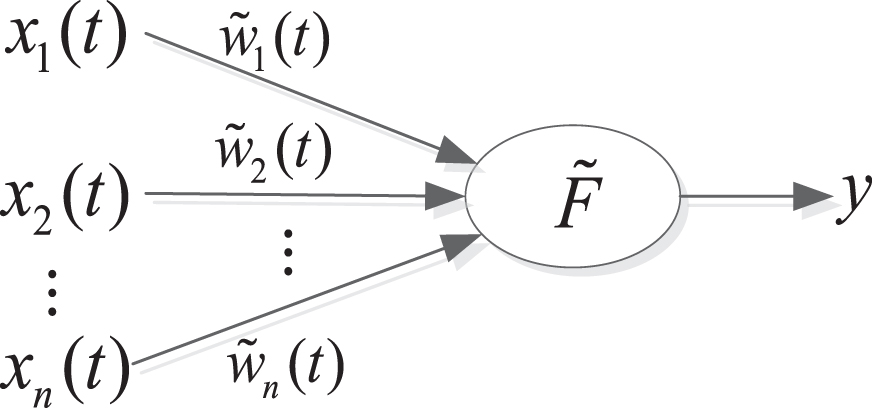
Fuzzy process neuron.

In Fig. 2,X (t) = (x₁ (t) , x₂ (t) , ⋯ , x (t)) represents process input signal of FPN in the interval [0, T], $\tilde{W} (t) = ({\tilde{w}}_{1} (t),$ ${\tilde{w}}_{2} (t), \dots, {\tilde{w}}_{n} (t))$ is the corresponding fuzzy connection weight function, y is the class output of the signal sample.

Define a generalized inner product operation that can measure similarity of the distribution characteristics between X₁ (t) and X₂ (t) in the interval[0, T]:

$< X_{1} (t), X_{2} (t) >) = \frac{\frac{1}{n} {(\sum_{i = 1}^{n} \int_{0}^{T} (x_{1 i} (t) x_{2 i} (t)) dt)}^{2}}{| | X_{1} (t) | | \cdot | | X_{2} (t) | |}$ (12)

The space-time dimensional aggregation operation of FPN is taken as the generalized inner product of the process signal X (t) and the fuzzy connection weight function $\tilde{W} (t)$ . The action function $\tilde{f}$ adopts function with fuzzy membership property, then the relationship between FPN input/output is: $\begin{matrix} \tilde{F} (X (t)) = \tilde{f} (< \tilde{W} (t), X (t) >) \\ = \tilde{f} (\frac{\frac{1}{n} {(\sum_{i = 1}^{n} \int_{0}^{T} ({\tilde{w}}_{i} (t) x_{i} (t)) dt)}^{2}}{| | X (t) | | \cdot | | \tilde{W} (t) | |}) \end{matrix}$ (13)

If the action function of FPN adopts exponential Sigmoid membership function: $g (x) = \frac{1}{1 + e^{- a (x - c)}}$ . Where, a, c are parameters determining function distribution. At this time, the input/output relationship of FPN is expressed as $\begin{matrix} \tilde{F} (X (t)) = \tilde{f} (< \tilde{W} (t), X (t) >) \\ = \frac{1}{1 + exp (- a (\int_{0}^{T} \sum_{i = 1}^{n} {\tilde{w}}_{i} (t) x_{i} (t) dt - c))} \end{matrix}$ (14)

In practical applications, based on the specific problems to be processed, FPN action function can also adopt other types of functions such as Gauss function, trigonometric function, bell-shaped function, composite membership degree, etc.

2.2.2 Fuzzy process neural network

The FPNN model constructed in this paper consists of four layers of information processing units. The first layer is the process signal input layer with n nodes; the second layer is FPN hidden layer, which is supposed to have m nodes and have full interconnection with the input layer. The fuzzy connection weight between the layer and the input layer is taken as a typical sample function of different subsets in the training set. The third layer is the model layer with K nodes (K is the number of classes of process signal in the training set), which selectively sums up the output of the FPN hidden layer based on class attribute corresponding to the FPN connection weight function. The fourth layer is the fuzzy linear classifier, which completes the classification of the input signal. The FPNN structure is shown in Fig. 3.

Fig. 3

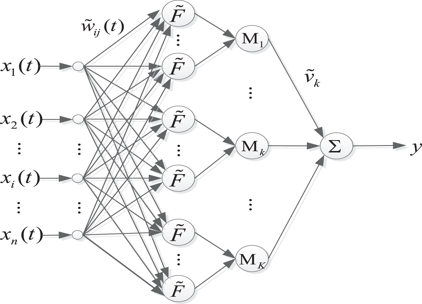
FPNN model.

In the process signal classification, for the representation and application of fuzzy process knowledge, this paper selects representative samples from different types of process signal sets, and uses its shape distribution characteristics and its combination relationship to implicitly express the fuzzy process knowledge of signal classes. Each type of signal set may consist of several typical samples, which are determined by experts subjectively or by using dynamic fuzzy clustering algorithm.

Suppose there are K model classes C_k, k = 1, 2, ⋯ , K in the training set; where, C_k consists of m_k typical sample functions denoted as z_kl (t)(l = 1, 2, ⋯ , m_k), the number of FPN hidden layer nodes is set as m = m₁ + m₂ + ⋯ + m_K. Therefore, the matrix of the connection weight function between the input layer and the FPN hidden layer has n × m dimensions, which is expressed as $\tilde{W} (t) = [{\tilde{w}}_{ij} (t)]_{n \times m}$ . The nodes of the FPN hidden layer and $\tilde{W} (t)$ are determined by the following method.

The m typical sample functions selected in the training set are sequentially ranked as z₁₁ (t) , ⋯ , z_1m₁ (t) , z₂₁ (t) , ⋯ , z_2m₂ (t) , ⋯, z_K1 (t) , ⋯ , z_{Km
_K} (t); where, the first subscript of z_kl (t)(l = 1, 2, ⋯ , m_k ; k = 1, 2, ⋯ , K) represents the class number of the signal sample, and the second subscript represents the l-th typical sample in the k-th model. Using z_ij (t) as the connection weight function from the input layer node i to the hidden layer node j, then the connection weight function between FPNN input layer and FPN hidden layer can then be determined. At this time, the selective summation of the FPN hidden layer output to the model layer node M_k is performed only by the class identifier k of z_kl (t).

If the input of FPNN is X (t) = (x₁ (t) , x₂ (t) , ⋯ , x_n (t)), and the action function of FPN is exponential Sigmoid function, then FPN hidden layer output H = [h₁, h₂, ⋯ , h_m] is calculated as

$\begin{matrix} h_{j} & = & \frac{1}{1 + exp (- a_{j} (\int_{0}^{T} \sum_{i = 1}^{n} {\tilde{w}}_{ij} (t) x_{i} (t) dt - c_{j}))}, \\ j = 1, 2, \dots, m \end{matrix}$ (15)

In formula (4-15),a_j and c_j are property parameters.

The output of FPNN model layer is $p_{k} = \sum_{j \in Ω_{k}} h_{j}, k = 1, 2, \dots, K$ (16)

In formula (4-16), K is the number of model classes included in the training set, Ω_k is the set of hidden layer node numbers corresponding to the k-th model.

From Fig. 3, the output of FPNN is $\begin{matrix} y = \sum_{k = 1}^{K} {\tilde{v}}_{k} p_{k} \\ = \sum_{k = 1}^{K} {\tilde{v}}_{k} \sum_{s \in Ω_{j}} \frac{1}{1 + exp (- a_{s} (\int_{0}^{T} \sum_{i = 1}^{n} {\tilde{w}}_{is} (t) x_{i} (t) dt - c_{s}))} \end{matrix}$ (17)

Where, ${\tilde{v}}_{k}$ is the fuzzy connection right from the model layer to the output layer.

Using the supervised learning method, the fuzzy classifier gives the output value of FPNN in the interval [0, 1]. The process input signals are classified in accordance with the decision principle that the actual output is closest to the expected output.

2.2.3 FPNN learning algorithm

Using supervised learning method, the FPNN learning process can be divided into three stages: First, the process signal is preprocessed considering the irregularity of the distribution pattern of the process signal. According to the statistical characteristics of the signal distribution, a set of appropriate standard orthogonal function bases are selected to represent the process signal in finite term expansion form of the set of function bases under a given fitting precision. Such processing not only facilitates FPNN calculation, but also achieves implicit representation of process signal distribution characteristics. Second, in the training set, the typical sample function of each model subclass is selected as the connection weight function of FPNN. Third, the connection weights between property parameters, model layer and output layer in FPN action function are optimally solved.

2.2.3.1
Expanded representation of process signal based on orthogonal function base Suppose b₁ (t),b₂ (t) , ⋯, b_l (t) , ⋯ is a set of standard orthogonal function bases in FPNN input space. For ∀X (t) = (x₁ (t) , x₂ (t) , ...,x_n (t))∈U (t), under the given fitting precision, x_i (t) can be expressed as: $x_{i} (t) = \sum_{l = 1}^{L} a_{il} b_{l} (t), i = 1, 2, \dots, n$ (18)

Where, L is the number of terms of the function base meeting the fitting precision requirement, a_il is the expansion coefficient corresponding to b_l (t).
2.2.3.2
Determination of typical signal samples in each model subclass of the sample set Two methods can be employed to determine typical signal samples in each model class of the sample set. The first is to analyze the distribution characteristics of signal samples and make empirical selection. The second is to take dynamic clustering algorithm, with the central function of each cluster as the typical sample. For the second case, this paper adopts the generalized Fréchet distance to measure the similarity of the distribution characteristics between process signals, and uses dynamic fuzzy C-means clustering algorithm to determine the typical samples of each signal model subclass.
2.2.3.2.1
Similarity measure of process signal distribution characteristics based on generalized Fréchet distance Fréchet distance is a distance measure for judging similarity between polygon curves. Suppose there are 2 given functions: f (t) : [0, 1] → R and g (t) : [0, 1] → R,the Fréchet distance between them is defined as follows: $d_{F} (f, g) = inf_{α, β} max_{t \in [0, 1]} dist (f (α (t)), g (β (t)))$ (19)

Where, α, β are continuous non-decreasing real functions, and α (0) = β (0) =0,α (1) = β (1) =1.

For time series signals, the discrete generalized Fréchet distance recursion is defined as follows:
For a polygonal chain P = < p₁, p₂, ⋯ , p_n> with n high points, there is a high point along k-walk segmentation of P, forming k disjoint non-empty subset {P_i} _i=1,⋯,k, which meets P_i =< p_{n_i-1+1}, ⋯ , p_{n
_i} > and 0 = n₀< n₁ < ⋯<n_k = n.

For two given polygon chains, A = < a₁, a₂, ⋯ , a_m >, B =< b₁, b₂, ⋯ , b_n >, the paired walk along A and B consists of k step {A_i} _i=1,⋯,k along A and k step {B_i} _i=1,⋯,k _along B, which makes either of A_i,B_i exactly contains a high point for 1 ⩽ i ⩽ k, i.e.|A_i| = 1, or|B_i| = 1.

The cost of paired walk of W = {(A_i, B_i)} along the chains A and B is defined as $d_{F}^{W} (A, B) = max_{i} max_{(a, b) \in A_{i} \times B_{i}} dist (a, b)$ (20)

Then, the discrete Fréchet distance between the chains A and B is $d_{F} (A, B) = min_{W} d_{F}^{W} (A, B)$ (21)
2.2.3.2.2
Dynamic fuzzy C-means clustering algorithm Fuzzy C-means clustering (FCM) represents a flexible classification algorithm, which views each cluster generated by clustering as a fuzzy set and determines clustering relationship by membership degree. In practical applications, FCM often encounters problems that the number of clusters is difficult to determine beforehand and there is sensitivity to initial values. In view of the above problems, this paper introduces granularity idea into FCM to establish a dynamic fuzzy C-means clustering algorithm. By calculating the coupling degree and resolution of the information granule, the clustering results are evaluated from different granular spaces, the optimized clustering results are selected, and the optimal clustering number is determined.

(1) Generalized density and initial clustering center

Suppose U (t) is the set of process signals, then the density at the sample point x_i (t) is defined as: $D_{i} = \sum_{k = 1}^{n} \frac{1}{1 + f_{d} | | x_{i} (t) - x_{k} (t) | |_{F}^{2}}, i = 1, 2, \dots, n$ (22)

Where, $| | \cdot | |_{F}^{2}$ is generalized Fréchet distance; $f_{d} = 4 / r_{d}^{2}$ , $r_{d} = \frac{1}{2} \sqrt{\frac{1}{n (n - 1)} \sum_{k = 1}^{n} \sum_{i = 1}^{n} | | x_{i} (t) - x_{k} (t) | |_{F}^{2}}$ is effective radius of the neighborhood density. A bigger D_i indicates that sample points surrounding x_i (t) are denser, and the density at x_i (t) is greater.

The density of each sample point in the sample set is calculated and the points in the low density area are deleted to obtain a sample set D in the high density area. The sample point with the highest density is selected from D as the first clustering center v₁ (t), and then the sample point farthest from v₁ (t) is selected from D as the second clustering center v₂ (t). Then, the distance between the remaining sample points in D and v₁ (t), v₂ (t) is calculated to find the minimum among them and the sample point of the maximum value is selected as the third clustering center v₃ (t). In a similar way, C initial clustering centers are selected.

Different clustering numbers are selected in sequence for clustering, and the results correspond to different partitions of the sample set. The partition result is evaluated by the degree of separation and coupling between samples. The degree of separation represents the separation between classes. The larger the term, the better the separation is. The degree of coupling indicates the compactness within the class. The smaller the term, the better the compactness is. Here, the degree of coupling is defined as.

$\begin{matrix} C_{d} (c) & = & \frac{1}{n} \sum_{i = 1}^{c} \sum_{j = 1}^{n} μ_{ij}^{m} d_{ij}^{2}; i = 1, 2, \dots, c, \\ j = 1, 2, \dots, n \end{matrix}$ (23)

The degree of separation is defined as: $S_{d} (c) = \frac{\sum_{i, k = 1; i \neq k}^{c} d_{ik}^{2}}{[c (c - 1)] / 2}; i, k = 1, 2, \dots, c$ (24)

The clustering results are evaluated using the following formula: $GD (c) = α C_{d} (b) + β \frac{1}{S_{d} (b)}; α + β = 1$ (25)

Where, α is weight factor of coupling degree, β is weight factor of separation degree, α is generally slightly larger than β.

For different cluster numbers, a smaller GD (c) value represents better clustering results, C value corresponding to the minimum value of GD (c) is the optimal cluster number, and its partition of the sample set leads to optimal clustering. Each clustering center function is selected as a typical signal sample of the sample set.
2.2.3.2.3
Solving FPNN model parameters For P given samples:(x_p1 (t) , x_p2 (t) , . . . , x_pn (t) , d_p), p = 1, 2, . . . , P; where, the first subscript of x_pi (t) represents the learning sample number, and the second subscript represents the input function vector component number; d_p is the network expectation output corresponding to the input x_p1 (t) , x_p2 (t) , ⋯ , x_pn (t).For the FPNN model shown in Fig. 3, the connection weight function from the input layer to the hidden layer is determined by the clustering center function of each model subclass in the sample set, and the parameters demanding adjustment include the weight ${\tilde{v}}_{k}$ from the model layer to the output layer and FPN hidden layer property parameters a_j, c_j. According to the principle of mean square error minimization, the error function isdefined as $E = \frac{1}{2} \sum_{p = 1}^{P} \sum_{k = 1}^{K} (d_{pk} - y_{pk})^{2}$ (26)

Based on gradient descent algorithm, Gradient descent algorithms of v_k and a_j, c_j are $- \frac{\partial E}{\partial v_{k}} = \sum_{p = 1}^{P} (d_{pk} - y_{pk})$ (27)

$\begin{matrix} - \frac{\partial E}{\partial a_{j}} & = & - 2 \sum_{p = 1}^{P} \sum_{k = 1}^{K} (d_{pk} - y_{pk}) v_{jk} h_{j} \\ \frac{1}{s_{j}^{3} (1 + exp (- a_{j} (\int_{0}^{T} \sum_{i = 1}^{n} w_{ij} (t) x_{i} (t) dt - c_{j})))} \end{matrix}$ (28)

$\begin{matrix} - \frac{\partial E}{\partial c_{j}} & = & - 2 \sum_{p = 1}^{P} \sum_{k = 1}^{K} (d_{pk} - y_{pk}) v_{jk} h_{j} \\ \frac{1}{s_{j}^{3} (1 + exp (- a_{j} (\int_{0}^{T} \sum_{i = 1}^{n} w_{ij} (t) x_{i} (t) dt - c_{j})))} \end{matrix}$ (29)

$v_{k} = v_{k} - α \frac{\partial E}{\partial v_{k}}; k = 1, 2, \dots, K$ (30)

$a_{j} = a_{j} - β \frac{\partial E}{\partial a_{j}}; j = 1, 2, \dots, m$ (31)

$c_{j} = c_{j} - γ \frac{\partial E}{\partial c_{j}}; j = 1, 2, \dots, m$ (32)

Where, α, βand γ mean learning efficiency, s_j is Sigmoid function value.
3 Actual data processing and result analysis

3.1 Prediction of impact hazard level of coal rock mass based on regularized fuzzy neural network

The regularized FNN method established in Section 2 of this paper is taken to predict the impact hazard level of coal rock mass. The regularized FNN integrates fuzzy logic reasoning, artificial neural network learning and classification discriminating ability. It is possible to use the structural geology, engineering mechanics parameters and mining factors to construct a FNN analysis model for prediction research on impact hazard level of coal rock mass. The impact hazard of coal rock mass is divided into four levels: none, slight, medium and severe.

According to the analysis data of coal mines and the results of expert interpretation, screening is performed according to class correction strategy for sample vector with close fuzzy membership function values. 76 typical samples of coal rock mass impact in 4 classes are selected as learning samples of fuzzy neural network training set.

The topological structure of the regularized fuzzy neural network is determined as 7-28-28-326-1, which means 7 input nodes, 28 fuzzy layer nodes (4 membership functions are correspondingly taken for each input), 28 regularization layer nodes, 326 rule layer nodes and 1 output layer node. The learning process of the network adopts single-sample cyclic error correction method. That is, one sample is randomly extracted from the sample set for network learning until the error precision is satisfied, and then the next sample is selected. Such loop iteration continues until all samples meet error precision requirement. The learning parameters are selected as follows: maximum learning times 15000, learning speed 0.65, inertia coefficient 0.45, learning precision 0.1 (the maximum deviation of actual output of each sample from desired output). In practice, the network training time is 6213 (76 samples are included each time to obtain correction meeting precision requirement).

The learned network is used for type recognition of other coal rock mass impact samples. In identification of 32 samples of the same mine, 25 samples were correctly judged, with recognition accuracy up to 78.1%. This represents a high precision in the automatic prediction of impact hazard of coal rock mass.

3.2 Prediction of coal rock mass impact based on fuzzy process neural network

To predict the impact hazard level of coal rock mass using the fuzzy process neural network method established in Section 3 of this paper, in terms of mechanism, it is possible to adaptively select representative typical samples and coal rock mass impact model under different geological conditions and mining modes as fuzzy process knowledge. The geostress monitoring data, microquake monitoring data, mining production daily footage data and cumulative footage data are time-aligned and used as index data for coal rock mass impact prediction. According to the data collected by the research group which include on-site analysis and expert interpretation results, 126 signal samples in 4 classes were selected as modeling data sets. Using dynamic fuzzy C-means clustering algorithm, it was determined that there were 3 typical models with strong impact, 4 typical models with general impact, 3 typical models with slight impact and 2 typical models without impact. By random selection based on proportion, 80 samples were selected as training set and 46 samples were selected as test set.

Using FPNN for coal rock mass impact hazard prediction requires a uniform process input interval. In practice, each signal sample generally has different recording time. The maximum time interval of all samples to be processed are rounded up and added by 1 to form a unified process interval. For samples with shorter time, a baseline value of 0.2 is taken for the deficient portion. At the same time, each indicator signal has different dimensions with big magnitude differences, so formula: x′ (t) = x (t) - min x (t)/ - max x (t) - min x (t) is used for normalization processing. Where, min x (t) and max x (t) are the minimum and maximum values of the time interval indicator.

The structural parameters of FPNN are selected as follows: the input layer has 4 process signal input nodes; the number of FPN hidden layer nodes is 12, which are ranked and labeled as 3 strong impact nodes, 4 general impact nodes, 3 slight impact nodes and 2 nodes with no impact. The connection weight function matrix from the input layer to the FPN hidden layer forms 12 typical sample function matrices, with connection mode consistent with the type and order of each node of the FPN hidden layer. Model layer has 4 nodes; fuzzy classifier has 1 output node. The normalized monitoring process data is expanded by legendre orthogonal function base at a fitting accuracy of 0.05. When the term number is 76, the fitting accuracy requirement is met. According to the algorithm in Section 3.3 of this paper, the property parameters and connection rights in FPNN are determined. The training error precision is set to 0.05, the maximum number of iterations is 5000, the learning efficiency is 0.45, and the membership function adopts exponential sigmoid function. FPNN is trained using 80 training samples, and the network converges after 3247 iterations. The test set samples were tested, and 37 of the 46 samples were accurately predicted, with accuracy of 80.2%.

4 Conclusion

In view of the problem of rock burst tendency prediction, a regularized fuzzy neural network for correlation numerical parameter analysis and a fuzzy process neural network model for process signal classification are proposed. The fuzzy neural network can fuse learning properties and classification mechanism of neural network for signal training sample features, and fuzzy logic system’s ability to express and decide on class knowledge, so that in mechanism, extraction, representation and information correlation of signal distribution features can be implemented. Seen from approximation ability of neural network, the algorithm can be viewed as a deterministic algorithm, but the hidden layer of the model adopts exponential action function with fuzzy membership meaning, which enables the model to have some features of the stochastic algorithm, so that inference structure of the whole model concords with T-S fuzzy decision method. FPNN can directly input process signals, which effectively broadens the scope of application of common fuzzy neural networks. Due to its few adjustable parameters and faster convergence, the model is suitable for real-time processing of information. The experimental results suggest that the two models and algorithms have good adaptability and certain application potential in predictive analysis of rock burst with uncertainty.

References

Xia

, Lan

and Wei

, Study of comprehensive evaluation technology for rock burst hazard based on microseismic and underground sound monitoring, Journal of China Coal Society 36(S2) (2011), 358–364.

Liu

Y.J.

, Lu

, Tong

, Chen

C.P.

and Liand

D.J.

, Adaptive control-based barrier Lyapunov functions for a class of stochastic nonlinear systems with full state constraints, Automatica 87 (2018), 83–93.

Qin

, Chen

, Li

, Sun

and Fu

, Evaluation model and application of rock burst coupling based on set pair analysis and interval triangular fuzzy number, Shandong University of Science and Technology (Natural Science) 38(1) (2019), 16–24.

Jin

, Wang

, Liu

, Huang

and Wang

, Catastrophe progression method on comprehensive evaluation of rock burst, Journal of Mining and Safety Engineering 30(2) (2013), 256–261.

, A Traffic Motion Object Extraction, Algorithm, International Journal of Bifurcation and Chaos 25(14) (2015), Article Number 1540039.

, Wang

and Zou

, Research on internet information mining based on agent algorithm, Future Generation Computer Systems 86 (2018), 598–602.

, Wang

and Yuntao

, Bidirectional cognitive computing method supported by cloud technology, Cognitive Systems Research 52 (2018), 615–621.

Wen

and Yu

, NRS-ACPSO-SVM based model for prediction of rock burst risk, China Safety Science Journal 27(10) (2017), 19–25.

Wen

, Chen

, Yang

, Dou

and Tian

, Research on prediction of rock burstbased on optimized Bagging-LSSVM model, China Safety Science Journal 27(6) (2017), 121–126.

10.

Wang

, Zhou

, Li

, Liu

and Wang

, A multi-parameter identification model for classification of rock burstrisk and its application, Journal of China Coal Society 42(S2) (2017), 311–322.

11.

Tang

and Xia

K.W.

, Seismological method for prediction of areal rockbursts in deep mine with seismic source mechanism and unstable failure theory, Journal of Central South University of Technology 17(5) (2010), 947–953.

12.

Liu

Y.J.

, Lu

, Tong

, et al., Adaptive control-based Barrier Lyapunov Functions for a class of stochastic nonlinear systems with full state constraints. Automatica 87 (2018), 83–93.

13.

Nayak

Puma C.

, et al., A neuro-fuzzy computing technique for modeling hydrological time series, Journal of Hydrology 291(1-2) (2004), 52–66.

14.

Gao

, Murphey

Y.L.

and Zhu

, Multivariate time series prediction of lane changing behavior using deep neural network, Applied Intelligence 48(10) (2018), 3523–3527 15.