Generalization of Seikkala derivative and differential transform method for fuzzy Volterra integro-differential equations

Abstract

In this study, we present a generalized concept of Seikkala differentiability for fuzzy functions. It has been shown that this concept and the lateral H-differentiability lead us to the same results. Fuzzy differential transform method (FDTM) is applied to solve fuzzy Volterra integro-differential equations. In order to show the effectiveness of this method some illustrative examples are given.

Keywords

Fuzzy derivative generalized Seikkala derivative fuzzy Volterra intego-differential equation fuzzy differential transform method

1 Introduction

Fuzzy differential equation is a very useful tool to model dynamical systems under possibilistic uncertainty [8]. The topic of fuzzy integral and integro-differential equations has been developed a lot in recent years [19 –25]. The solutions of fuzzy differential, integral and integro-differential equations have a major role in the fields of science and engineering [9 –11]. When a physical system is modeled, it finally gives a differential, an integral or an intero-differential equation.

There are lots of different types of differentiability in the literature. In 1983, Puri and Ralescu first introduce the concept of Hukuhara differentiability [2]. The approach based on the Hukuhara derivative has the disadvantage that a differentiable function has increasing length of its support interval [32]. This is not always a realistic assumption. If g : (a, b) → R is differentiable on x₀ ∈ (a, b) with g′ (x₀) <0, then f (x) = c . g (x) , ∀ x ∈ (a, b) where c is a fuzzy number, is not Hukuhara differentiable. This is a big shortcoming of Hukuhara derivative. Then in 1987S. Seikkala introduces Seikkala derivative [3]. Seikkala derivative is actually defined by one of the property by Hukuhara derivative and both the derivative signifies the same. Although the definition of Seikkala derivative is easier to understand than the definition of Hukuhara derivative but it has the same disadvantages as the Hukuhara derivative. So in 2005 Bede and Gal [14] introduce strongly generalized differentiability and weakly generalized differentiability of fuzzy number valued function. These two concepts of differentiability solve the above mentioned shortcoming of Hukuhara and Seikkala derivative but these have a disadvantage compared to Hukuhara and Seikkala derivative that is a fuzzy differential equation has no unique solution. Then L. Stefanini and B. Bede [16] introduce fuzzy gH-derivative which coincides with the concept of weakly generalized differentiability. Again Bede and Stefanini [17] introduce another concept of fuzzy derivative, fuzzy g-derivative, which is the most general among the previous definitions. In fact fuzzy gH-derivative and fuzzy g-derivative coincide whenever gH-difference exists. Since, in the last two cases of strongly generalized differentiability, the derivative is trivial because it is reduced to crisp element. There are other works also on fuzzy derivative [5, 33] where they redefine fuzzy derivative by considering fist two cases of strongly generalized differentiability and neglect last two cases of strongly generalized differentiability. Barros and Pedro [12] introduce a new concept of fuzzy derivatives, interactive derivatives, by using interactive fuzzy differences.

Lots of work has been done to solve fuzzy integral and integro-differential equations [4 , 26–31]. There are very few works on numerical solution of fuzzy Volterra integro-differential equations. Here we have used FDTM which is an analytical-numerical and computer programming friendly technique that depends on Taylor series. DTM was first introduced by Zhou with an application in electrical circuits [15]. In this paper, generalized Seikkala derivative has been introduced and its properties have been given in Section 3. FDTM and its properties have been given in Section 4. Finally illustrative examples and a brief conclusion are provided.

2 Preliminaries

Definition 2.1. Let E be the set of all upper semi continuous normal convex fuzzy numbers with bounded α-cut intervals. It means if v ∈ E then the α-cut set is a closed bounded interval which is denoted by $v_{α} = [v_{1}, v_{2}] .$

For arbitrary u_α = [u₁, u₂] , v_α = [v₁, v₂] and k ≥ 0, addition (u_α + v_α) and multiplication by k are defined as $\begin{matrix} (u + v)_{1} (α) & = & u_{1} (α) + v_{1} (α), (u + v)_{2} (α) \\ = & u_{2} (α) + v_{2} (α), (ku)_{1} (α) \\ = & {ku}_{1} (α), (ku)_{2} (α) = {ku}_{2} (α) \end{matrix}$ and each y ∈ R can be regarded as a fuzzy number defined by $μ_{y} (x) = {\begin{matrix} 1 if x = y, \\ 0 if x \neq y . \end{matrix}$

The Hausdorff distance between fuzzy numbers given by D : E × E → R⁺ ∪ {0} $\begin{matrix} D (u, v) & = & sup max {| u_{1} (α) - v_{1} (α) |, \\ | u_{2} (α) - v_{2} (α) |}, α \in [0, 1] \end{matrix}$

It is easy to see that D is a metric in E and has the following properties (see [4])

D (u ⊕ w, v ⊕ w) = D (u, v) , ∀ u, v, w ∈ E,

D (k ⊙ u, k ⊙ v) = |k|D (u, v) , ∀ k ∈ R, u, v ∈ E

D (u ⊕ v, w ⊕ e) ≤ D (u, w) + D (v, e) , ∀ u, v, w, e ∈ E,

(D, E) is a complete metric space.

Definition 2.2. (see [1]) Let f : R → E be a fuzzy valued function. If for arbitrary fixed t₀ ∈ R and ɛ > 0, ∃ a δ > 0 such that |t - t₀| < δ ⇒ D (f (t) , f (t₀)) < ɛ, f is said to be continuous.

Definition 2.3. (see [2]) Let x, y ∈ E. If there exist z ∈ E such that x = y + z, then z is called the H-difference of x and y and it is denoted by x ⊖ y .

Definition 2.4. (see [2]) A function f : (a, b) → E is called H-differentiable on x₀ ∈ (a, b) if for h > 0 sufficiently small there exist the H-differences f (x₀ + h) ⊖ f (x₀) , f (x₀) ⊖ f (x₀ - h) and an element f′ (x₀) ∈ E such that $\begin{matrix} lim_{x \to 0} \frac{f (x_{0} + h) ⊖ f (x_{0})}{h} \\ = lim_{x \to 0} \frac{f (x_{0}) ⊖ f (x_{0} - h)}{h} \\ = f^{'} (x_{0}) \end{matrix}$

Definition 2.5. (see [3]) The S-derivative (Seikkala derivative) at x₀ ∈ (a, b) of a fuzzy-number-valued function f : (a, b) → E is defined by $f_{α}^{'} (x_{0}) = [f_{1}^{'} (x_{0}, α), f_{2}^{'} (x_{0}, α)], 0 \leq α \leq 1$ provided that it defines a fuzzy number f′ (x₀) ∈ E .

Definition 2.6. (see [5]) Let f : (a, b) → E and x₀ ∈ (a, b). One says f is (1)-differentiable at x₀, if there exists an element f′ (x₀) ∈ E such that for all h > 0 sufficiently small there exist f (x₀ + h) ⊖ f (x₀) , f (x₀) ⊖ f (x₀ - h) and the limits (in the metric D) $lim_{x \to 0^{+}} \frac{f (x_{0} + h) ⊖ f (x_{0})}{h} = lim_{x \to 0^{+}} \frac{f (x_{0}) ⊖ f (x_{0} - h)}{h} = f^{'} (x_{0}) .$ f is (2)-differentiable at x₀, if there exists an element f′ (x₀) ∈ E such that for all h < 0 sufficiently small there exist f (x₀ + h) ⊖ f (x₀) , f (x₀) ⊖ f (x₀ - h) and the limits (in the metric D) $\begin{matrix} lim_{x \to 0^{-}} \frac{f (x_{0} + h) ⊖ f (x_{0})}{h} \\ = lim_{x \to 0^{-}} \frac{f (x_{0}) ⊖ f (x_{0} - h)}{h} \\ = f^{'} (x_{0}) . \end{matrix}$

3 Generalized Seikkala derivative

Let f : (a, b) → E and the functions f₁ (x, α) and f₂ (x, α) are continuously differentiable with respect to x, uniformly continuous with respect to α ∈ [0, 1] . Then f is H-differentiable if and only if it is S-differentiable and the two derivatives coincide (see Remark 8.27 in [6]). So, S-derivative and H-derivative has the same shortcoming which has been solved by introducing strongly generalized derivative in [14] which is same as Definition 2.6. This shortcoming can be also solved by introducing generalized concept of S-differentiability as follows.

Definition 3.1. Let f : (a, b) → E and x₀ ∈ (a, b) . Then the generalized Seikkala derivative (gS-derivative) of f (x) at x₀ is denoted f′ (x₀) and defined by

if $f_{1}^{'} (x_{0}, α), f_{2}^{'} (x_{0}, α)$ exist and $f_{1}^{'} (x_{0}, α) \leq f_{2}^{'} (x_{0}, α)$ then $f_{α}^{'} (x_{0}) : = [f_{1}^{'} (x_{0}, α), f_{2}^{'} (x_{0}, α)]$

if $f_{1}^{'} (x_{0}, α), f_{2}^{'} (x_{0}, α)$ exist and $f_{1}^{'} (x_{0}, α) \geq f_{2}^{'} (x_{0}, α)$ then $f_{α}^{'} (x_{0}) : = [f_{2}^{'} (x_{0}, α), f_{1}^{'} (x_{0}, α)]$

Remark 3.1. This gS-derivative is well-defined because if f (x) is gS-differentiable at x₀ ∈ [a, b] in the form of (i) and (ii) both then $f_{1}^{'} (x_{0}, α) = f_{2}^{'} (x_{0}, α)$ i.e. f′ (x₀) ∈ R ⊂ E .

Theorem 3.1. The following definitions of derivative are equivalent

lateral H-derivatives (Definition 2.6)

generalized S-derivative (Definition 3.1)

Proof. Let f : (a, b) → E is lateral H-differentiable. Then according to Theorem 5 in [5] f₁ (x, α) and f₂ (x, α) are differentiable and if f (x) is (1)-differentiable then $f_{α}^{'} (x) = [f_{1}^{'} (x, α), f_{2}^{'} (x, α)]$ i.e. f (x) is gS-differentiable in the form of (i) or if f (x) is (2)-differentiable then $f_{α}^{'} (x) = [f_{2}^{'} (x, α), f_{1}^{'} (x, α)]$ i.e. f (x) is gS-differentiable in the form of (ii). Therefore (a) implies (b).

Let f : (a, b) → E is gS-differentiable in the form of (i) then f₁ (x, α) , f₂ (x, α) exist, $f_{1}^{'} (x, α) \leq f_{2}^{'} (x, α)$ and $f_{α}^{'} (x) = [f_{1}^{'} (x, α), f_{2}^{'} (x, α)]$ (1)

Therefore, $\begin{matrix} lim_{x \to 0^{+}} \frac{f_{1} (x + h, α) - f_{1} (x, α)}{h} \\ = lim_{x \to 0^{+}} \frac{f_{1} (x, α) - f_{1} (x - h, α)}{h} = f_{1}^{'} (x, α) . \end{matrix}$ (2) $\begin{matrix} lim_{x \to 0^{+}} \frac{f_{2} (x + h, α) - f_{2} (x, α)}{h} \\ = lim_{x \to 0^{+}} \frac{f_{2} (x, α) - f_{2} (x - h, α)}{h} = f_{2}^{'} (x, α) . \end{matrix}$ (3) $\begin{matrix} lim_{x \to 0^{+}} \frac{f_{1} (x + h, α) - f_{1} (x, α)}{h} \\ \leq lim_{x \to 0^{+}} \frac{f_{2} (x + h, α) - f_{2} (x, α)}{h} \end{matrix}$ (4) $\begin{matrix} lim_{x \to 0^{+}} \frac{f_{1} (x, α) - f_{1} (x - h, α)}{h} \\ \leq lim_{x \to 0^{+}} \frac{f_{2} (x, α) - f_{2} (x - h, α)}{h} \end{matrix}$ (5)

Therefore from (4) we get

$\begin{matrix} lim_{x \to 0^{+}} \frac{f (x + h) ⊖ f (x)}{h} \\ = [lim_{x \to 0^{+}} \frac{f_{1} (x + h, α) - f_{1} (x, α)}{h}, \\ lim_{x \to 0^{+}} \frac{f_{2} (x + h, α) - f_{2} (x, α)}{h}] exists \end{matrix}$ (6) and from (5) we get

$\begin{matrix} lim_{x \to 0^{+}} \frac{f (x) ⊖ f (x - h)}{h} \\ = [lim_{x \to 0^{+}} \frac{f_{1} (x, α) - f_{1} (x - h, α)}{h}, \\ lim_{x \to 0^{+}} \frac{f_{2} (x, α) - f_{2} (x - h, α)}{h}] exists . \end{matrix}$ (7)

Now using (1)-(3) in (6) and (7) we get

$\begin{matrix} lim_{x \to 0^{+}} \frac{f (x + h) ⊖ f (x)}{h} \\ = lim_{x \to 0^{+}} \frac{f (x) ⊖ f (x - h)}{h} = f^{'} (x) . \end{matrix}$ (8)

Hence f (x) is (1)-differentiable. Similarly we can prove that if f (x) is gS-differentiable in the form of (ii) then f (x) is (2)-differentiable. Therefore (b) implies (a), which completes the proof.

Remark 3.2. From the above theorem we can say that the theorems and properties true for lateral H-derivative is also true for gS-derivative and those theorems and properties can also be proved by using the definition of gS-derivative.

4 Fuzzy differential transform method (FDTM)

Definition 4.1. The transformation F (k) of kth derivative of a function f (x) : (a, b) → E in one variable is as follows:

$\begin{matrix} F_{1} (k, α) & = & \frac{1}{k!} [\frac{d^{k} f_{1} (x, α)}{{dx}^{k}}]_{x = 0}, \\ F_{2} (k, α) & = & \frac{1}{k!} {[\frac{d^{k} f_{2} (x, α)}{{dx}^{k}}]}_{x = 0}, \\ \forall k \in {0, 1, 2, \dots} \end{matrix}$ (9) when f (x) is gS-differentiable in the form of (i) and $\begin{matrix} F_{1} (k, α) & = & \frac{1}{k!} {[\frac{d^{k} f_{2} (x, α)}{{dx}^{k}}]}_{x = 0}, \\ F_{2} (k, α) & = & \frac{1}{k!} {[\frac{d^{k} f_{1} (x, α)}{{dx}^{k}}]}_{x = 0}, k is odd, \end{matrix}$ (10) $\begin{matrix} F_{1} (k, α) & = & \frac{1}{k!} {[\frac{d^{k} f_{1} (x, α)}{{dx}^{k}}]}_{x = 0}, \\ F_{2} (k, α) & = & \frac{1}{k!} {[\frac{d^{k} f_{2} (x, α)}{{dx}^{k}}]}_{x = 0}, k is even, \end{matrix}$ (11) when f (x) is gS-differentiable in the form of (ii).

So, if f (x) be gS-differentiable in the form of (i) then f (x) can be presented as follows: $f_{1} (x, α) = \sum_{k = 0}^{\infty} (x - x_{0})^{k} F_{1} (k, α),$ (12) $f_{2} (x, α) = \sum_{k = 0}^{\infty} (x - x_{0})^{k} F_{2} (k, α),$ (13) and if f (x) be gS-differentiable in the form of (ii) then f (x) can be presented as follows: $\begin{matrix} f_{1} (x, α) & = & \sum_{k = 0, even}^{\infty} (x - x_{0})^{k} F_{1} (k, α) \\ + \sum_{k = 1, odd}^{\infty} (x - x_{0})^{k} F_{2} (k, α), \end{matrix}$ (14) $\begin{matrix} f_{2} (x, α) & = & \sum_{k = 0, even}^{\infty} (x - x_{0})^{k} F_{2} (k, α) \\ + \sum_{k = 1, odd}^{\infty} (x - x_{0})^{k} F_{1} (k, α) . \end{matrix}$ (15)

Theorem 4.1. Let us consider f (x) , u (x) and v (x) are fuzzy valued functions and their fuzzy differential transformations denoted by F (k) , U (k) and V (k) , respectively. If f (x) , u (x) and v (x) are all gS-differentiable in the form (i) or all gS-differentiable in the form of (ii). Then

if f (x) = u (x) + v (x) , then $F (k) = U (k) + V (k), k \in {0, 1, 2, \dots}$

if f (x) = u (x) - v (x) , then $F (k) = U (k) - V (k), k \in {0, 1, 2, \dots}$

if f (x) = u (x) ⊖ v (x) , then $F (k) = U (k) ⊖ V (k), k \in {0, 1, 2, \dots}$

Proof. Using the Definition 4.1 the proof is obvious.

Theorem 4.2. Let us consider f (x) , u (x) and v (x) are fuzzy valued functions and their fuzzy differential transformations denoted by F (k) , U (k) and V (k) , respectively. If f (x) , u (x) are (i)-differentiable and v (x) is (ii)-differentiable or f (x) , u (x) are (ii)-differentiable and v (x) is (i)-differentiable then

if f (x) = u (x) + v (x) , then $F (k) - V (k) = U (k), k \in {0, 1, 2, \dots}$

if f (x) = u (x) - v (x) , then $F (k) = U (k) ⊖ V (k), k \in {0, 1, 2, \dots}$

if f (x) = u (x) ⊖ v (x) , then $F (k) = U (k) - V (k), k \in {0, 1, 2, \dots}$

Proof. Using Definition 4.1 the proof is obvious.

Theorem 4.3. Let us consider the fuzzy-valued functions g (x) ∈ E where g (x) is gS-differentiable

in the form of (i) and $f (x) = \int_{x_{0}}^{x} g (t) dt,$ then $F (k) = \frac{G (k - 1)}{k},$ k ≥ 1 where F (k) and G (k) are the fuzzy differential transformations of f and g respectively.

Proof. From Theorem 3.2 of [7] this result is true for (1)-differentiable. Therefore using Theorem 3.1 we can say that this result is true for gS-differentiable in the form of (i).

Theorem 4.4. Let us consider the fuzzy-valued functions g (x)∈ E where g (x) is gS-differentiable in the form of (ii) and $f (x) = \int_{x_{0}}^{x} g (t) dt,$ then for 0 ≤ α ≤ 1 and k ≥ 1

$\begin{matrix} F_{1} (k, α) & = & {\begin{matrix} \frac{G_{1} (k - 1, α)}{k}, k = 1, 3, \dots \\ \frac{G_{2} (k - 1, α)}{k}, k = 2, 4, \dots \end{matrix} \\ F_{2} (k, α) & = & {\begin{matrix} \frac{G_{2} (k - 1, α)}{k}, k = 1, 3, \dots \\ \frac{G_{1} (k - 1, α)}{k}, k = 2, 4, \dots \end{matrix} \end{matrix}$ where F (k) and G (k) are the fuzzy differential transformations of f and g respectively.

Proof. Using the definition of FDTM, we get for 0 ≤ α ≤ 1

$\begin{matrix} f_{α} (x) & = & \int_{x_{0}}^{x} g_{α} (t) dt = [\int_{x_{0}}^{x} g_{1} (t, α) dt, \int_{x_{0}}^{x} g_{2} (t, α) dt] \\ = & [\int_{x_{0}}^{x} (\sum_{k = 0, even}^{\infty} (t - x_{0})^{k} G_{1} (k, α) + \sum_{k = 1, odd}^{\infty} (t - x_{0})^{k} G_{2} (k, α)) dt, \\ \int_{x_{0}}^{x} (\sum_{k = 0, even}^{\infty} (t - x_{0})^{k} G_{2} (k, α) + \sum_{k = 1, odd}^{\infty} (t - x_{0})^{k} G_{1} (k, α)) dt] \\ = & [\sum_{k = 0, even}^{\infty} \frac{(x - x_{0})^{k + 1}}{k + 1} G_{1} (k, α) + \sum_{k = 1, odd}^{\infty} \frac{(x - x_{0})^{k + 1}}{k + 1} G_{2} (k, α), \\ \sum_{k = 0, even}^{\infty} \frac{(x - x_{0})^{k + 1}}{k + 1} G_{2} (k, α) + \sum_{k = 1, odd}^{\infty} \frac{(x - x_{0})^{k + 1}}{k + 1} G_{1} (k, α)] \end{matrix}$

Now changing the index we have $\begin{matrix} = [\sum_{k = 1, odd}^{\infty} \frac{(x - x_{0})^{k}}{k} G_{1} (k - 1, α) + \sum_{k = 2, even}^{\infty} \frac{(x - x_{0})^{k}}{k} G_{2} (k - 1, α), \\ \sum_{k = 1, odd}^{\infty} \frac{(x - x_{0})^{k}}{k} G_{2} (k - 1, α) + \sum_{k = 2, even}^{\infty} \frac{(x - x_{0})^{k}}{k} G_{1} (k - 1, α)] \end{matrix}$

Now by using Definition 4.1 we have $\begin{matrix} F (0, α) & = & 0 \\ F_{1} (k, α) & = & {\begin{matrix} \frac{G_{1} (k - 1, α)}{k}, k = 1, 3, \dots \\ \frac{G_{2} (k - 1, α)}{k}, k = 2, 4, \dots \end{matrix} \\ F_{2} (k, α) & = & {\begin{matrix} \frac{G_{2} (k - 1, α)}{k}, k = 1, 3, \dots \\ \frac{G_{1} (k - 1, α)}{k}, k = 2, 4, \dots \end{matrix} \end{matrix}$

Theorem 4.5. (see [7]) Let us consider the fuzzy-valued functions g (x) ∈ E where g (x) is (1)-differentiable and $f (x) = \int_{x_{0}}^{x} \int_{x_{0}}^{x_{n - 1}} \dots \dots \int_{x_{0}}^{x_{2}} \int_{x_{0}}^{x_{1}} g (t) {dtdx}_{1} {dx}_{2} \dots \dots {dx}_{n - 1},$ then $F (k) = \frac{(k - n)!}{k!} G (k - n),$ k ≥ n where F (k) and G (k) are the fuzzy differential transformations of f and g respectively.

Theorem 4.6. Let us consider the fuzzy-valued functions g (x) ∈ E where g (x) is gS-differentiable in the form of (ii) and

$f (x) = \int_{x_{0}}^{x} \int_{x_{0}}^{x_{n - 1}} \dots \dots \int_{x_{0}}^{x_{2}} \int_{x_{0}}^{x_{1}} g (t) {dtdx}_{1} {dx}_{2} \dots \dots {dx}_{n - 1},$ then for 0 ≤ α ≤ 1 and k ≥ n if n is an even number

$\begin{matrix} F_{1} (k, α) \\ = {\begin{matrix} \frac{(k - n)!}{k!} G_{2} (k - n, α), k = n + 1, n + 3, \dots \\ \frac{(k - n)!}{k!} G_{1} (k - n, α), k = n, n + 2, \dots \end{matrix} \\ F_{2} (k, α) \\ = {\begin{matrix} \frac{(k - n)!}{k!} G_{1} (k - n, α), k = n + 1, n + 3, \dots \\ \frac{(k - n)!}{k!} G_{2} (k - n, α), k = n, n + 2, \dots \end{matrix} \end{matrix}$ if n is an odd number $\begin{matrix} F_{1} (k, α) = \frac{(k - n)!}{k!} \\ {\begin{matrix} G_{2} (k - n, α), k = n + 1, n + 3, \dots \\ G_{1} (k - n, α), k = n, n + 2, \dots \end{matrix} \\ F_{2} (k, α) = \frac{(k - n)!}{k!} \\ {\begin{matrix} G_{1} (k - n, α), k = n + 1, n + 3, \dots \\ G_{2} (k - n, α), k = n, n + 2, \dots \end{matrix} \end{matrix}$

Proof. Using the definition of FDTM, we get for 0 ≤ α ≤ 1 $\begin{matrix} f_{1} (x, α) \\ = \int_{x_{0}}^{x} \int_{x_{0}}^{x_{n - 1}} \dots \dots \int_{x_{0}}^{x_{2}} \int_{x_{0}}^{x_{1}} g_{1} (t, α) {dtdx}_{1} {dx}_{2} \\ \dots \dots {dx}_{n - 1} \\ = \int_{x_{0}}^{x} \int_{x_{0}}^{x_{n - 1}} \dots \dots \int_{x_{0}}^{x_{2}} \int_{x_{0}}^{x_{1}} \sum_{k = 0, even}^{\infty} \\ (t - x_{0})^{k} G_{1} (k, α) \\ + \sum_{k = 1, odd}^{\infty} (t - x_{0})^{k} G_{2} (k, α) {dtdx}_{1} {dx}_{2} \\ \dots \dots {dx}_{n - 1} \\ = \sum_{k = 0, even}^{\infty} \frac{(t - x_{0})^{k + n}}{(k + 1) (k + 2) \dots (k + n)} G_{1} (k, α) \\ + \sum_{k = 1, odd}^{\infty} \frac{(t - x_{0})^{k + n}}{(k + 1) (k + 2) \dots (k + n)} G_{2} (k, α) \end{matrix}$ and $\begin{matrix} f_{2} (x, α) \\ = \int_{x_{0}}^{x} \int_{x_{0}}^{x_{n - 1}} \dots \dots \int_{x_{0}}^{x_{2}} \int_{x_{0}}^{x_{1}} g_{2} (t, α) {dtdx}_{1} {dx}_{2} \\ \dots \dots {dx}_{n - 1} \\ = \int_{x_{0}}^{x} \int_{x_{0}}^{x_{n - 1}} \dots \dots \int_{x_{0}}^{x_{2}} \int_{x_{0}}^{x_{1}} \sum_{k = 0, even}^{\infty} (t - x_{0})^{k} \\ G_{2} (k, α) \\ + \sum_{k = 1, odd}^{\infty} (t - x_{0})^{k} G_{1} (k, α) {dtdx}_{1} {dx}_{2} \\ \dots \dots {dx}_{n - 1} \\ = \sum_{k = 0, even}^{\infty} \frac{(t - x_{0})^{k + n}}{(k + 1) (k + 2) \dots (k + n)} G_{2} (k, α) \\ + \sum_{k = 1, odd}^{\infty} \frac{(t - x_{0})^{k + n}}{(k + 1) (k + 2) \dots (k + n)} G_{1} (k, α) \end{matrix}$

Now if n is even, then after changing the index we have $\begin{matrix} f_{1} (x, α) \\ = \sum_{k = n, even}^{\infty} \frac{(k - n)!}{k!} (t - x_{0})^{k} G_{1} (k - n, α) \\ + \sum_{k = n + 1, odd}^{\infty} \frac{(k - n)!}{k!} (t - x_{0})^{k} G_{2} (k - n, α) \\ f_{2} (x, α) \\ = \sum_{k = n, even}^{\infty} \frac{(k - n)!}{k!} (t - x_{0})^{k} G_{2} (k - n, α) \\ + \sum_{k = n + 1, odd}^{\infty} \frac{(k - n)!}{k!} (t - x_{0})^{k} G_{1} (k - n, α) \end{matrix}$

Therefore, for 0 ≤ α ≤ 1 and k ≥ n $\begin{matrix} F_{1} (k, α) \\ = {\begin{matrix} \frac{(k - n)!}{k!} G_{2} (k - n, α), k = n + 1, n + 3, \dots \\ \frac{(k - n)!}{k!} G_{1} (k - n, α), k = n, n + 2, \dots \end{matrix} \\ F_{2} (k, α) \\ = {\begin{matrix} \frac{(k - n)!}{k!} G_{1} (k - n, α), k = n + 1, \dots \\ \frac{(k - n)!}{k!} G_{2} (k - n, α), k = n, n + 2, \dots \end{matrix} \end{matrix}$

Now if n is even, then after changing the index we have $\begin{matrix} f_{1} (x, α) \\ = \sum_{k = n, odd}^{\infty} \frac{(k - n)!}{k!} (t - x_{0})^{k} G_{1} (k - n, α) \\ + \sum_{k = n + 1, even}^{\infty} \frac{(k - n)!}{k!} (t - x_{0})^{k} G_{2} (k - n, α) \\ f_{2} (x, α) \\ = \sum_{k = n, odd}^{\infty} \frac{(k - n)!}{k!} (t - x_{0})^{k} G_{2} (k - n, α) \\ + \sum_{k = n + 1, even}^{\infty} \frac{(k - n)!}{k!} (t - x_{0})^{k} G_{1} (k - n, α) \end{matrix}$

Therefore, for 0 ≤ α ≤ 1 and k ≥ n $\begin{matrix} F_{1} (k, α) = \frac{(k - n)!}{k!} \\ {\begin{matrix} G_{2} (k - n, α), k = n + 1, n + 3, \dots \\ G_{1} (k - n, α), k = n, n + 2, \dots \end{matrix} \\ F_{2} (k, α) = \frac{(k - n)!}{k!} \\ {\begin{matrix} G_{1} (k - n, α), k = n + 1, n + 3, \dots \\ G_{2} (k - n, α), k = n, n + 2, \dots \end{matrix} \end{matrix}$

Theorem 4.7. (see [7]) Suppose that U (k) and G (k) are the differential transformation of the functions u (x) (is a fuzzy valued function) and g (x) (is a positive real-valued function), respectively. If $f (x) = \int_{x_{0}}^{x} g (t) u (t) dt$ then under (1)-differentiability of f we have for 0 ≤ α ≤ 1 and k ≥ 1 $\begin{matrix} F_{1} (k, α) & = & \sum_{l = 0}^{k - 1} G (l) \frac{U_{1} (k - l - 1, α)}{k}, \\ F_{2} (k, α) & = & \sum_{l = 0}^{k - 1} G (l) \frac{U_{2} (k - l - 1, α)}{k}, \end{matrix}$ and under (2)-differentiability of f we have for 0 ≤ α ≤ 1 and k ≥ 1 $\begin{matrix} F_{1} (k, α) & = & \sum_{l = 0, even}^{k - 1} G (l) \frac{U_{1} (k - l - 1, α)}{k} \\ + \sum_{l = 0, odd}^{k - 1} G (l) \frac{U_{2} (k - l - 1, α)}{k}, \\ F_{2} (k, α) & = & \sum_{l = 0, even}^{k - 1} G (l) \frac{U_{2} (k - l - 1, α)}{k} \\ + \sum_{l = 0, odd}^{k - 1} G (l) \frac{U_{1} (k - l - 1, α)}{k} . \end{matrix}$

Theorem 4.8. (see [7]) Suppose that U (k) and G (k) are the differential transformation of the functions u (x) (is a fuzzy valued function) and g (x)(is a positive real-valued function), respectively. If $f (x) = g (x) \int_{x_{0}}^{x} u (t) dt,$ then under (1)-differentiability of f we have for 0 ≤ α ≤ 1 and k ≥ 1 $\begin{matrix} F_{1} (k, α) & = & \sum_{l = 0}^{k - 1} G (l) \frac{U_{1} (k - l - 1, α)}{k - 1}, \\ F_{2} (k, α) & = & \sum_{l = 0}^{k - 1} G (l) \frac{U_{2} (k - l - 1, α)}{k - 1}, \end{matrix}$ and under (2)-differentiability of f we have for 0 ≤ α ≤ 1 and k ≥ 1 $\begin{matrix} F_{1} (k, α) & = & \sum_{l = 0, even}^{k - 1} G (l) \frac{U_{1} (k - l - 1, α)}{k - 1} \\ + \sum_{l = 0, odd}^{k - 1} G (l) \frac{U_{2} (k - l - 1, α)}{k - 1}, \\ F_{2} (k, α) & = & \sum_{l = 0, even}^{k - 1} G (l) \frac{U_{2} (k - l - 1, α)}{k - 1} \\ + \sum_{l = 0, odd}^{k - 1} G (l) \frac{U_{1} (k - l - 1, α)}{k - 1} . \end{matrix}$

Theorem 4.9. (see [7]) Suppose that U (k) and G (k) are the differential transformation of the functions u (x) (is a fuzzy valued function) and g (x) (is a positive real-valued function), respectively. If f (x) = g (x) u (x), then under (1)-differentiability of f we have $F (k, α) = \sum_{l = 0}^{k} G (l) U (k - l, α), 0 \leq α \leq 1 .$

Theorem 4.10. Let us consider the fuzzy-valued functions g (x) ∈ E and $f (x) = \frac{d^{n} g (x)}{{dx}^{n}} .$

If g (x) is gS-differentiable in the form of (i) then $F (k) = \frac{(k + n)!}{k!} G (k + n)$

If g (x) is gS-differentiable in the form of (ii) then if n is even, $F (k) = \frac{(k + n)!}{k!} G (k + n)$ and if n is odd, $F_{1} (k) = \frac{(k + n)!}{k!} G_{2} (k + n)$ and $F_{2} (k) = \frac{(k + n)!}{k!} G_{1} (k + n) .$

Proof. The proof is obvious from Definition 4.1.

5 Applications and numerical results

In this section, we apply the present method on some test problems. The numerical results are calculated using Wolfram Mathematica 9.0 and the figures are drawn using MATLAB R2010a. One can see from the numerical results, by increasing approximating terms, the accuracy of the approximate solution increases.

In order to perform a superior error analysis of the obtained approximate solutions by our method, we use the following convergence indicator

The point wise absolute error:

$E_{i}^{K} (x, α) = | u_{i}^{exact} (x, α) - u_{i, K}^{A} (x, α) |,$ where

FDT is considered up to k = K .

Problem 5.1. Let us consider the following nonlinear fuzzy Volterra integro-differential equation $u " (x) = f (x) + \frac{1}{2} \int_{0}^{x} u^{2} (t) d t,$ where $f_{α} (x) = (1 + x + x^{2}) [α, 2 - α]$ with initial conditions $u_{α} (0) = [α, 2 - α], u_{α}^{'} (0) = [1 + α, 3 - α] .$

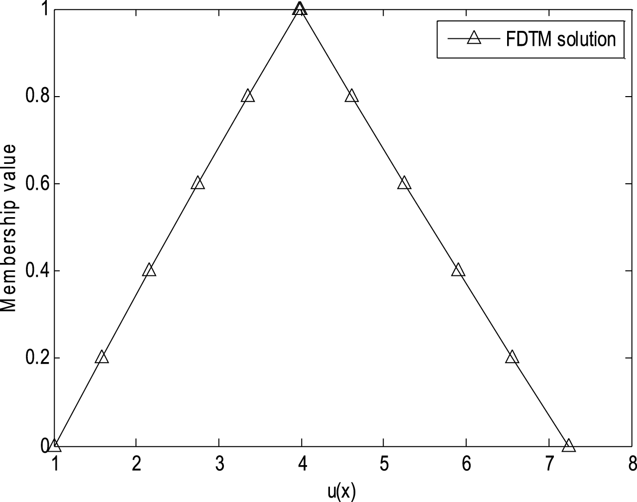
Now using the properties of FDTM we have the result for 0 ≤ α ≤ 1, k = 0 $\begin{matrix} U_{1} (k + 2, α) \\ = \frac{1}{(k + 1) (k + 2)} [{δ (k) + δ (k - 1) \\ + δ (k - 2)} α], \\ U_{2} (k + 2, α) \\ = \frac{1}{(k + 1) (k + 2)} [{δ (k) + δ (k - 1) \\ + δ (k - 2)} (2 - α)], \end{matrix}$ and for k > 0 $\begin{matrix} U_{1} (k + 2, α) \\ = \frac{1}{(k + 1) (k + 2)} [{δ (k) + δ (k - 1) + δ (k - 2)} α \\ + \frac{1}{2 k} \sum_{l = 0}^{k - 1} U_{1} (l, α) U_{1} (k - l - 1, α)], \\ U_{2} (k + 2, α) \\ = \frac{1}{(k + 1) (k + 2)} [{δ (k) + δ (k - 1) \\ + δ (k - 2)} (2 - α) \\ + \frac{1}{2 k} \sum_{l = 0}^{k - 1} U_{1} (l, α) U_{1} (k - l - 1, α)] . \end{matrix}$

Then after considering FDT up to k = 7 we get an approximate Taylor series solution of order 7 as follows $\begin{matrix} u_{1, 7}^{A} (x, α) \\ = α + (1 + α) x + \frac{α}{2} x^{2} + \frac{α^{2} + 2 α}{12} x^{3} \\ + \frac{α^{2} + 3 α}{24} x^{4} + \frac{2 α^{2} + 2 α + 1}{120} x^{5} \\ + \frac{7 α^{3} + 2 α^{2} + 6 α}{1440} x^{6} + \frac{6 α^{3} + 9 α^{2} + 4 α}{5040} x^{7} \\ + o (8) \\ u_{1, 7}^{A} (x, α) \\ = (2 - α) + (3 - α) x + \frac{2 - α}{2} x^{2} \\ + \frac{α^{2} - 6 α + 8}{12} x^{3} + \frac{α^{2} - 7 α + 10}{24} x^{4} \\ + \frac{2 α^{2} - 10 α + 13}{120} x^{5} \\ + \frac{- α^{3} + 14 α^{2} - 50 α + 52}{1440} x^{6} \\ + \frac{- α^{3} + 15 α^{2} + 48 α + 44}{5040} x^{7} + o (8) \end{matrix}$

The graph of the membership function of the solution of Problem 5.1 is given in Fig. 1. From Fig. 1 we can see that as the initial conditions of the Problem 5.1 are given by triangular fuzzy number, the solution of the Problem 5.1 also represents a triangular fuzzy number.

Fig.1

FDTM solution for the membership function at x = 1 for Problem 5.1.

Problem 5.2. Let us considered here a linear fuzzy Volterra integro-differential equation as $\begin{matrix} u^{″} (x) & = & a (1 + x) + \int_{0}^{x} (x - t) u (t) dt, where \\ a_{α} = [α, 2 - α] \end{matrix}$ subject to the initial conditions $u_{α} (0) = [α, 2 - α], u_{α}^{'} (0) = [α, 2 - α]$

The exact solution, given by classical solution method, is u₁ = αe^x and u₂ = (2 - α) e^x.

By the same application of the FDTM which is used for Problem 5.1, the approximating solutions can be obtained for different values of K.

Now after considering FDT up to k = 7 we get an approximate Taylor series solution of order 7 as follows $\begin{matrix} u_{1, 7}^{A} (x, α) & = & α (1 + x + \frac{x^{2}}{2!} + \frac{x^{3}}{3!} + \frac{x^{4}}{4!} \\ + \frac{x^{5}}{5!} + \frac{x^{6}}{6!} + \frac{x^{7}}{7!}) + o (8) \\ u_{2, 7}^{A} (x, α) & = & (2 - α) (1 + x + \frac{x^{2}}{2!} + \frac{x^{3}}{3!} + \frac{x^{4}}{4!} \\ + \frac{x^{5}}{5!} + \frac{x^{6}}{6!} + \frac{x^{7}}{7!}) + o (8) \end{matrix}$

Hence $\begin{matrix} lim_{x \to \infty} u_{1, K}^{A} (x, α) & = & α e^{x} = u_{1} \\ lim_{x \to \infty} u_{2, K}^{A} (x, α) & = & (2 - α) e^{x} = u_{2} \end{matrix}$

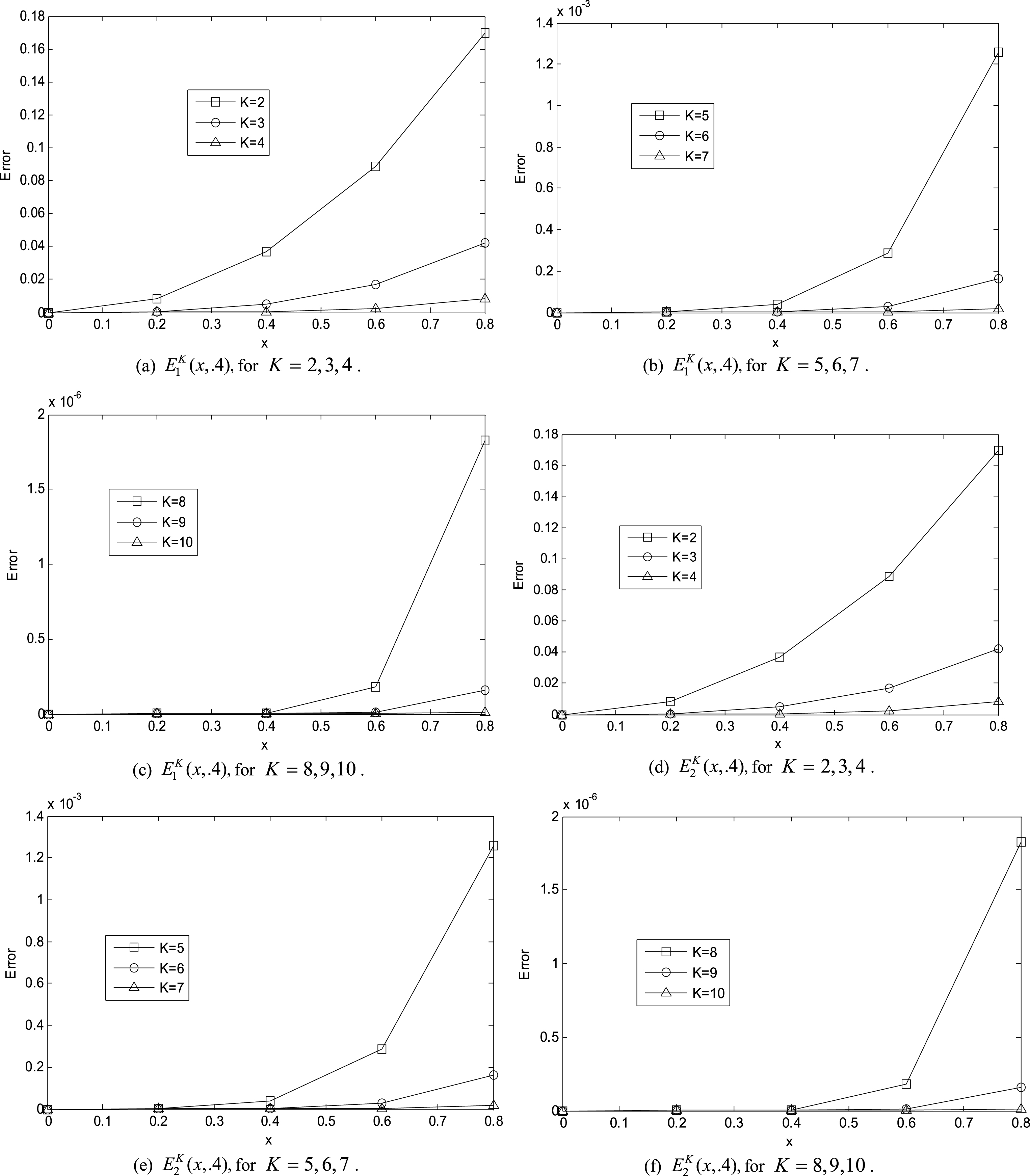
The absolute point wise errors of obtained values by our method for different number of approximating terms are shown in Table 1 and Table 2. Figure 2 shows the physical behavior of the absolute error function. As one can see from Fig. 2, by increasing the value of K, the absolute error functions approach to zero very rapidly. Besides, Fig. 2 also shows that our FDTM gives reasonable results for small K too.

Fig.2

The behavior of the absolute values of error functions versus x, and different values of the approximating terms, K for Problem 5.2.

Table 1

Absolute point wise errors of obtain values by our method for different values of K for Problem 5.2

X	$E_{1}^{4} (x, . 4)$	$E_{1}^{8} (x, . 4)$	$E_{2}^{4} (x, . 4)$	$E_{2}^{8} (x, . 4)$
0.0	0.00E-00	0.00E-00	0.00E-00	0.00E-00
0.2	2.78E-05	3.66E-08	2.78E-05	2.60E-11
0.4	4.63E-04	2.41E-06	4.63E-04	6.80E-09
0.6	2.45E-03	2.83E-05	2.45E-03	1.78E-07
0.8	8.08E-03	1.64E-04	8.08E-03	1.83E-06
1.0	2.06E-02	6.46E-04	2.06E-02	1.11E-05

Table 2

Absolute point wise errors of obtain values by our method for different values of K for Problem 5.2

x	$E_{1}^{4} (x, . 8)$	$E_{1}^{8} (x, . 8)$	$E_{2}^{4} (x, . 8)$	$E_{2}^{8} (x, . 8)$
0.0	0.00E-00	0.00E-00	0.00E-00	0.00E-00
0.2	5.55E-05	5.19E-11	8.33E-05	7.79E-11
0.4	7.93E-04	1.36E-09	1.39E-03	2.04E-08
0.6	4.90E-03	3.57E-07	7.34E-03	5.35E-07
0.8	1.62E-02	3.65E-06	2.42E-02	5.48E-06
1.0	4.13E-02	2.23E-05	6.19E-02	3.34E-05

Problem 5.3. Following Ref. [27], let us consider the fuzzy Volterra integro-differential equation as $\begin{matrix} u^{'} (x) & = & f (x) + \int_{0}^{x} (x^{2} + t^{2}) u (t) dt, where \\ f_{α} & = & [\frac{1}{12} α x^{2} (α^{4} + 2) (36 - 5 x^{4}), \\ \frac{1}{4} x^{2} (α^{3} - 2) (5 x^{4} - 36)] \end{matrix}$ subject to the initial conditions $u_{α} (0) = [α, 2 - α], u_{α}^{'} (0) = [α, 2 - α]$

The exact solution is $u_{1} (x, α) = (α^{5} + 2 α) x^{3} and u_{2} = (6 - 3 α^{3}) x^{3}$

By the same application of the FDTM which is used for Problem 5.1, the approximating solutions can be obtained for different values of K.

Now after considering FDT up to k = 3 we get the exact solution $\begin{matrix} u_{1, 3}^{A} (x, α) & = & (α^{5} + 2 α) x^{3} and \\ u_{2, 3}^{A} (x, α) & = & (6 - 3 α^{3}) x^{3} \end{matrix}$

Table 3 and Table 4 show the comparison of absolute point wise error, which are obtain by our method for K = 3, Variational Iteration Method (VIM) [27] for number of iterations, n + 1 =3 and Homotopy Perturbation Method (HPM) [27] for number of iterations = 3 . One can see from Tables 3 and 4 that although the VIM [27] gives more accurate result than HPM [27] but our method, FDTM, is more accurate and quicker than these methods.

Table 3

Comparison of absolute errors between our method (DTM), VIM [27] and HPM [27] for Problem 5.3

VIM [27]	HPM [27]	Our Method(DTM)
α	$E_{1}^{3} (\frac{1}{2}, α)$	$E_{1}^{3} (\frac{1}{2}, α)$	$E_{1}^{3} (\frac{1}{2}, α)$
0.0	0.0000E-00	0.0000E-00	0.0000E-00
0.1	7.6675E-11	2.5125E-06	0.0000E-00
0.2	1.5347E-10	5.0288E-06	0.0000E-00
0.3	2.3095E-10	7.5676E-06	0.0000E-00
0.4	3.1061E-10	1.0178E-05	0.0000E-00
0.5	3.9534E-10	1.2954E-05	0.0000E-00
0.6	4.8984E-10	1.6051E-05	0.0000E-00
0.7	6.0113E-10	1.9698E-05	0.0000E-00
0.8	7.3899E-10	2.4215E-05	0.0000E-00
0.9	9.1641E-10	3.0029E-05	0.0000E-00
1.0	1.1501E-09	3.7686E-05	0.0000E-00

Table 4

Comparison of absolute errors between our method (DTM), VIM [27] and HPM [27] for Problem 5.3

VIM [27]	HPM [27]	Our Method (DTM)
α	$E_{2}^{3} (\frac{1}{2}, α)$	$E_{2}^{3} (\frac{1}{2}, α)$	$E_{2}^{3} (\frac{1}{2}, α)$
0.0	2.3001E-09	7.5371E-05	0.0000E-00
0.1	2.2990E-09	7.5333E-05	0.0000E-00
0.2	2.2909E-09	7.5070E-05	0.0000E-00
0.3	2.2691E-09	7.4354E-05	0.0000E-00
0.4	2.2265E-09	7.2959E-05	0.0000E-00
0.5	2.1564E-09	7.0660E-05	0.0000E-00
0.6	2.0517E-09	6.7231E-05	0.0000E-00
0.7	1.9057E-09	6.2444E-05	0.0000E-00
0.8	1.7113E-09	5.6076E-05	0.0000E-00
0.9	1.4617E-09	4.7899E-05	0.0000E-00
1.0	1.1501E-09	3.7686E-05	0.0000E-00

6 Conclusions

In this work, the concept of gS-derivative has been introduced which is equivalent to the lateral H-derivative but compare to the definition of the lateral H-derivative, gS-derivative is more easy to understand and use. Therefore, gS-derivative gives an alternative way to define fuzzy derivative and to prove the properties of fuzzy derivative. Several properties of FDT are studied and FDTM for the solution of fuzzy Volterra integro-differential equation is nicely presented. We have explained the practicality and efficiency of this method by examining several numerical examples and the obtained results shows valuable performance over existing methods. In Problems 5.2 and 5.3 we have seen that if the exact solution of the fuzzy Volterra integro-differential equation exists then the solution given by our method converges to the exact solution very rapidly. Comparison with other numerical algorithms shows that our method, FDTM, gives better results compare to the VIM [27] and HPM [27]. For the VIM [27] and HPM [27] it is almost impossible to identify the exact solution, if it exists, by observing the approximate solution. Since, in our FDTM, the approximate solution is given in the form of Taylor series, if the exact solution exist then it is very easy to identify the exact solution by observing the approximate solution in the form of Taylor series of known function as we have seen in Problem 5.2.

Footnotes

Acknowledgments

The research work of Suvankar Biswas is financed by Department of Science and Technology, (No. DST/INSPIRE/Fellowship/2014/148) Govt. of India.

References

Mizukoshi

M.T.

, Barros

L.C.

, Chalco-Cano

, Roman-Flores

and Bassanezi

R.C.

, Fuzzy differential equations and extension principle, Information Sciences 177 (2007), 3627–3635.

Puri

and Ralescu

, Differentials of fuzzy functions, J Math Anal Appl 91 (1983), 552–558.

Seikkala

, On the fuzzy initial value problem, Fuzzy and Systems 24 (1987), 319–330.

Babolian

, SadeghiGoghary

and Abbasbandy

, Numerical solution of linear Fredholm fuzzy integral equations of the second kind by Adomian method, Applied Mathematics and Computation 161 (2005), 733–744.

Chalco-Cano

and Romn-Flores

, On new solutions of fuzzy differential equations, Chaos, Solitons and Fractals 38 (2008), 112–119.

Bede

, Mathematics of Fuzzy Sets and Fuzzy Logic, Springer, 2013, pp. 157–158.

Salahshour

and Allahviranloo

, Application of fuzzy differential transform method for solving fuzzy Volterra integral equations, Applied Mathematical Modelling 37 (2013), 1016–1027.

Zadeh

, Toward a generalized theory of uncertainty (GTU) – an outline, Information Sciences 175 (2005), 1–40.

Casasnovas

and Rossell

, Averaging fuzzy biopolymers, Fuzzy Sets and Syst 152 (2005), 139–158.

10.

Barros

L.C.

, Bassanezi

R.C.

and Tonelli

P.A.

, Fuzzy modelling in population dynamics, Ecol Model 128 (2000), 27–33.

11.

El Naschie

M.S.

, From experimental quantum optics to quantum gravity via a fuzzy Khler Manifold, Chaos, Solitons and Fractals 25 (2005), 969–977.

12.

Barros

L.C.

and Pedro

F.S.

, Fuzzy differential equations with interactive derivative, Fuzzy Sets and Systems 309 (2017), 64–80.

13.

Subrahmanyam

P.V.

and Sudarsanam

S.K.

, A note on fuzzy Volterra integral equations, Fuzzy Sets and Systems 81 (1996), 237–240.

14.

Bede

and Gal

S.G.

, Generalizations of differentiability of fuzzy-number-valued functions with applications to fuzzy differential equations, Fuzzy Sets and Systems 151 (2005), 581–599.

15.

Zhou

J.K.

, Differential Transformation and its application for electrical circuits, Huazhong University Press, Wuhan, China, 1986.

16.

Bede

and Stefanini

, Generalized Hukuhara differentiability of interval-valued functions and interval differential equations, Nonlinear Analysis 71 (2009), 1311–1328.

17.

Bede

and Stefanini

, Generalized differentiability of fuzzy-valued functions, Fuzzy Sets and Systems 230 (2013), 119–141.

18.

Bede

and Gal

S.G.

, Quadrature rules for integrals of fuzzy-number-valued functions, Fuzzy Sets Syst 145 (2004), 359–380.

19.

Mosleh

and Otadi

, Existence of solution of nonlinear fuzzy Fredholm integro-differential equations, Fuzzy Information and Engineering 8 (2016), 17–30.

20.

Zeinali

, Shahmorad

and Mirnia

, Fuzzy intrego-differential equations: Discrete solution and error estimation, Iranian Journal of Fuzzy Systems 10 (2013), 107–122.

21.

Mirzaee

and Hoseini

S.F.

, Solving systems of linear Fredholm integro-differential equations with Fibonacci polynomials, Ain Shams Engineering Journal 5 (2014), 271–283.

22.

Alikhani

, Bahrami

and Jabbari

, Existence of global solutions to nonlinear fuzzy Volterra integro-differential equations, Nonlin Anal 75 (2012), 1810–1821.

23.

Attari

and Yazdani

, A computational method for fuzzy Volterra Fredholm integral equations, Fuzzy Inf Eng 2 (2011), 147–156.

24.

Khorasani Kiasari

S.M.

, Khezerloo

, Dogani Aghcheghloo

M.H.

, Numerical solution of Linear Fredholm fuzzy integral equations by modified homotopy perturbation method, Aust J Basic Appl Sci 4 (2010), 6416–6423.

25.

Molabahrami

, Shidfar

and Ghyasi

, Ananalytical method for solving linear Fredholm fuzzy integral equations of the second kind, Comput Math Appl 61 (2011), 2754–2761.

26.

Abbasbandy

, Babolian

and Alavi

, Numerical method for solving linear Fredholm fuzzy Integral equations of the second kind, Chaos Solitons Fractals 31(1) (2007), 138–146.

27.

Matinfar

, Ghanbari

and Nuraei

, Numerical solution of linear fuzzy Volterra integro-differential equations by variational iteration method, Journal of Intelligent & Fuzzy Systems 24 (2013), 575–586.

28.

Allahviranloo

, Abbasbandy

, Sedaghatfar

and Darabi

, A new method for solving fuzzy integro-differential equation under generalized differentiability, Neural Computing and Applications 21 (2012), 191–196.

29.

Behzadi

S.S.

, Allahviranloo

and Abbasbandy

, Fuzzy collocation methods for second-order fuzzy Abel-Volterra integro-differential equations, Iranian Journal of Fuzzy Systems 11(2) (2014), 71–88.

30.

Allahviranloo

, Amirteimoori

, Khezerloo

and Khezerloo

, A new method for solving fuzzy Voltra integro-differential equations, Journal of Australian Journal of Basic and Applied Sciences 5(4) (2011), 154–164.

31.

Behzadi

Sh.S.

, Allahviranloo

and Abbasbandy

, Solving fuzzy second-order nonlinear Volterra–Fredholm integro-differential equations by using Picard method, Journal of Neural Computing & Applications 21(1) (2012), 337–346.

32.

Diamond

, Stability and periodicity in fuzzy differential equations, IEEE Transactions on Fuzzy Systems 8 (2000), 583–590.

33.

Chalco-Cano

and Roman-Flores

, Comparation between some approaches to solve fuzzy differential equations, Fuzzy Sets and Systems 160 (2009), 1517–1527.