A comparative review of optimisation techniques in segmentation of brain MR images

Abstract

MRI image segmentation, a challenging task in medical diagnostics aids in extracting the summarized information of the anatomy of the human brain, thereby offering the potentiality for accurate treatment of the disease. The purpose of this work is to elevate the performances of different optimization techniques that are used in automated segmentation procedures. The performance of four algorithms was evaluated quantitatively over the genetic algorithm-based segmentation, which is the prevailing approach in automated segmentation. The upshot exhibits the accuracy and performance of various optimization techniques with a genetic algorithm.

Keywords

Genetic algorithm harmonic mean magnetic resonance imaging SVM PSO TLBO

1 Introduction

Image segmentation is one of the rudimentary techniques in drawing out the contours of the image by which recognition of the objects in the image is made less complicated as stated by [27] Sudipta Roy Samir Kumar Bandyopadhyay, [14] Kailash Sinha and G.R. Sinha. In common, the assessment of segments involving user assistance approaches that involves techniques like supervised evaluation and subjective evaluation of the segments. Apart from the challenges of supervised based approach, it is obligatory to automate the segmentation that minimised the burden of the radiologist and more over the unsupervised based approach lean to generate accurate results as it works with a dynamic range of an image.

In [1], Nandhi and [18] Nursuriati Jamil et al. has proposed a morphological operations basedapproach, D. Selvaraj, R. Dhanasekaran [4] has proposed an approach intensity based on thresolding. Noha EI et al. in the article [17] has suggested a semi-automated technique through graph cuts segmentation approach in which the value of pixel distance is measured from the edges to designate them to the suitable segment. But the distance based methods may hardly converge towards the best possible number of segments in case of a wrongly chosen centroid and how ever the pixels are to delegated by considering the degree of belongingness through membership rather than the distance.

Geng-cheng et al. in his paper [9] had proposed a seeded region growing approach for automated segmentation of brain MRI images, but this mechanism has a considerable limitation in picking the initial seed point, especially in case of a noise image If the initial seed point is incorrect, it doesn’t yield a worthy outcome. And the technique is susceptible to initial seed point.

In the article [6], Goshal et al. had performed segmentation of the MRI image through a watershed technique that it is very accurate for segmentation of large images with numerous segments but the main pit fall of this technique is that many of the times it leads to over segmentation which is not appropriate for segmentation of the brain images as the MRI image constitutes brain fluids, tissues, and neurons which are recognised with different intensities and over segmentation. Under such circumstances, it may not fetch the best results. P. Singh et al. in the article [20], segmenting the MRI through Fuzzy C Means(FCM) algorithm that is efficient in semi-automated segmentation of MR image but the computational time for FCM is exceptionally high, As it need to evaluate the membership of each pixel with respect to cluster centers for pixel assignment.

As proposed by Angelina et al. in the article [24], the automated way of segmenting the MRI image for the non-invasive way involves more efficient techniques like region growing and region merging which is more liable to the initial seed points.And the objective function for the seed point identification would also be moderately complicated that needs to be more robust enough.

The paper is organized as section-II Image preprocessing to banish the salt and pepper noise, section-III presents stages of automated segmentation and Section IV presents about the genetic algorithm based variable string length based clustering, Section-V presents the work of Support vector Machine for optimisation, Section-VI presents the working of Particle swam optimisation for refining the segmented Section-VII presents the working of Teacher Learner Based Optimization. Section VIII is for data analysis of the MRI brain image segmentation utilising divergent optimisation approaches and exacting results of the different optimisation techniques. And section IX is the Conclusion and Section 10 is about the Future Scope.

2 Image preprocessing to eliminate salt and pepper noise

While the MRI image is being transformed, there is a chance of salt and pepper noise added to the image, as stated by K. V. R. Teja et al. in [13]. If any such image is segmented without performing preprocessing it may lead to misinterpretation. So the image has to be preprocessed before segmentation of the image.

Images with salt and pepper noise Q. Chen, in [21], will have the extreme intensity values either 255(Bright) representing the salt noise or 0(dark) representing the pepper noise. Here we use a 3×3 scanning technique to get the intensity of center pixel m(i, j) $p (i, j) = | m (i + x, j + y) - m (i, j) |$ (1)

When (i + x, j + y) ≠ (i, j) and p (i, j) gives the luminance difference. Now we recover the pixel intensity using the harmonic mean by using the following formula $r (i, j) = | p (i, j) - a (i, j) | / c$ (2)

r(i, j) recovered pixel, and a(i, j) is the average of 4 connected pixels and c is the weighted constant.

3 Stages of automated image segmentation

In general, a complete automated tumor diagnosis system CAD(computer aided diagnostics) is distantly accurate in terms of tumor estimation under certain initial assumptions, but for more accuracy, results the results could be further refined through the evolutionary algorithms. Automated image segmentation involves the following strategy for the identification of lesions and tumors. In the initial stage, the image is preprocessed to detach the noise, and then the features were extracted based on which the segmentation is progressed, and the obtained segments were assumed to be the initial clusters. The pixels are considered as initial population, and further refinement is performed for accurate identification of tumor/damaged index in the brain by further iterating it as shown in Fig. 1.

Fig.1

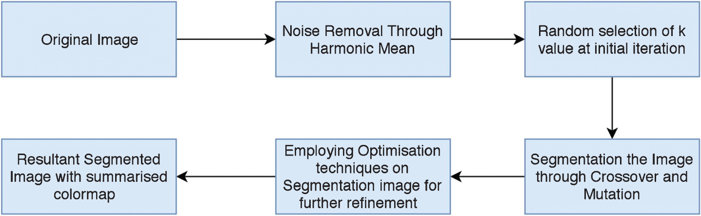
Block diagram of the segmentation procedure follows commonly in all the procedures.

4 Genetic algorithm based variable string length clustering

Image segmentation could be fruitful and effective through automated image segmentation technique. The automated approaches would automatically assess the appropriate number of segments through the genetic algorithm as ststed by Nicoara et al. [16] and. In this mechanism, a variable string length based approach, as stated by Chou et al. in the article [3], Das S., [5] and KarimaBenatchba, MouloudKoudil [15] has deployed Genetic Algorithm for segmenting the image in their work. The degree of belongingness of the assigning to the concerning segment would be decided by applying line symmetry based approach by making use of an index. And hence, in each iteration, the index value has been optimised to outreach the global best solution. It folds a variable number of image segments, i.e. the optimal value of K. However, the algorithm could be implemented on the cluster of diverse size and shape as stated by Singh Vijendra, Sahoo Laxman, in the article [26].

4.1 Selection operator

The Selection operator decides the individual elements, i.e., segments that are selected for crossover purpose based on the computed fitness value. Then the chromosomes are continuously updated through the fitness of an individual in each iteration. Finally, the number of copies of a chromosome that goes into the mating pool for subsequent operations is proportional to its fitness.

4.2 Crossover operation

Crossover operation is executed among a group of parent chromosome to produce a child chromosome as an offspring. The Crossover probability is a ratio that determines the number of chromosomes that will be selected to perform the crossover operation. The crossover probability would be reduced as the number of iteration were increased with the idea that the best chromosomes, i.e., segments, would remain the same and would propagate to the next generation.

The Line symmetric distanced as stated by Sriparna saha in the article [25], where ls(z, c) over a symmetric point be Z, and the relative center is C is set by 2 × C - Z and this is denoted by Z*. Let the Knear neighbors of Z* could be located at a Euclidean distance of des = 1, 2, 3, 4 ... ..Knear. Then $d_{ls} (z, c) = d_{sym} (z, c) x d_{ed} (z, c)$ (3) $d_{ls} (z, c) = \frac{\sum_{i = 1}^{k_{near}} d_{i}}{knear} x d_{ed} (z, c)$ (4)

Where d_ed(z,c) will be the Euclidean interval from the point Z to the center C. And d_sym, constitute line symmetric measure. However, from the above equation, it is drawn that the I value of ‘i’ lies between 1 and the best Knear value. So the knear value which we are going to choose must be optimal. In the case of 1, there will be no influence on Euclidean distance and incase the uppermost value is too large then it may lead to a un-deterministic state. Hence the upper bound is chosen close to 2. Knear value is hugely rely on the population distribution.

4.3 Mutation operation

After crossover operation is performed the pixels are assigned based on the point symmetric approach, and then mutation is performed on the resultant chromosomes of crossover based on mutation probability (0.01), that is proportion of the maximum likeness that an arbitrary elements of considered chromosome that would be flipped into a new set of chromosome for the next iteration.

5 Least squares support vector machine based automated MRI segmentation

SVM is one of the numerous supervisory learning approaches as experimented by X. Wang et al. [29], J. Xiao and Y. Tong [12] employed in generalised linear classification, SVM could be employed in optimising the segmentation by classifying the pixels among multiple segments and assigning them to the best optimal closest segment. Initially, the image with a random K number of segments is obtained by assigning the pixels to the centroid, which is a closest by line symmetric distance. Support vector machine will maximise the predictive accuracy at the same time avowing the over fit of data. Support Vector Machine could be defined as a mechanism that uses theoretical scope of a linear function a multi-dimensional feature space that working on the top of the trained image from an optimisation theory which is driven by statistical learning theory.

In SVM based MRI image segmentation as ststed by Fahd Mohsen et al. in the article [7] and I.Lizarazo. in the article [11], training samples are acquired, and the various dimensions were identified. From the identified set of dimensions, a few features were considered like intensity, texture or a boundary pixel and then based on the features the entire image is segmented. SVM need the training images, as much the algorithm is trained, the more the accuracy in segmentation. In the training phase, the decision function to decide the pixels fitness among the segments is evaluated by f(x,d,w) is given by $f (x, d, w) = \sum_{p = 0}^{n} d_{p} x_{p} + w$ (5)

From the equation, w is the weighted constant. And d is the dimension, i.e. the features that each pixel holds and xpis the Pth pixel in the segment.

Support Vector Machine aims in estimating the crucial point the hyper plane that maximises the least gap between any two pixel centroids. The equation for the hyper plane could be given as the following through quadratic equation

$\begin{matrix} Hp = \sum_{k = 0}^{n} P_{k} - 0.5 \times \sum_{k = 0}^{n} \sum_{l = 0}^{n} P_{k} \\ \times P_{l} \times Q_{k} \times Q_{l} \times C (R_{k}, R_{l}) \end{matrix}$ (6)

Under the rule, the value of $\sum_{k = 0}^{n} P_{k} P_{l} = 0$ . and the value of Pk lies between 0 and some constant Z for non-separable classes. R_k is corresponding to some training set and R_l is related to the corresponding class label.

6 Particle swarm optimisation for refinement of segmented image

Particle swarm optimisation is one of the prominent approaches as experimented by S. Ait-Aoudia et al. [23] and VasupradhaVijay et al. [28] in optimisation mechanisms. It an ideology influenced by the group of birds flying in search of food where the destination is not exactly known, but in every iteration, they converge towards the piece of food. In each iteration, a new particle is selected based on the p_best which is assumed to be the local best value and the g_best which is assumed to be the global best value that picks the best value among all the particles. The same assumptions are applied to the pixel segments for further optimisation of the segmented image for better results.

In PSO, everything we assumed as a swarm and particles, where a swarm is a group of particles which is applied in image segmentation by assuming the image segment which is resultant of variable string length based segmentation and each swarm consists of seed points with X coordinate and Y coordinate. And the resultant segmented image is further upgraded through computed fitness function that decides the g_best. In each iteration, the velocities and vectors are updated. The above said procedure is repeated until the stopping criteria are attained where no further bounces from the segment.

The PSO algorithm retains to reduces the ambiguity of boundary and unallocated pixels and maximises the number of segmented regions as follows $fun (seg) = W 1 * (P_{n} / P_{xi}) + W 2 * (S_{n} / S_{i})$ (7)

Where

W₁, W₂: Represents the weights for the function.

P_n: Represents the number of pixels in the image

P_xi: Represents the number of assigned pixels to the ith particle.

S_n: Represents the number of seeding points

S_i: Represents the number of segmented regions.

In some scenarios, when the fitness function is evaluated, the pixel may be shared by more than one segmented region that leads to inappropriate regions that are too large or too small. To address such a situation the above discussed equation is further optimised as below

$\begin{matrix} {opt}_{f} un (seg) = W 1 * (P_{n} / P_{xi}) \\ + W 2 * (S_{n} / \sum_{r = 1}^{S_{n}} C * N_{r}) \end{matrix}$ (8)

Where

N_r: Is the representation for a number of pixels in the region ‘r’.

C: Is decided as follows

C (v) = 1 if P_min < v < P_max

else 0 otherwise.

Upon conducting multiple iterations to optimise the solution, the global best solution at the final iteration is picked to be the best result.

6.1 Refining the resultant segmented image through PSO

In particle swam optimisation, the resultant segmented image of the genetic algorithm is further optimised by identifying the centroid pixel within the swam, i.e. in the segment and the fitness is computed for every pixel in the segment. The pixel which is having the highest fitness is the current iteration is assumed as the local best and based on the threshold value the pixels in the same segment are repositioned. Few pixels will be rescheduled to other segment based on the distance from the centroids of the neighboring segments. This is practiced for a few iterations until the stopping criteria are achieved.

7 Teacher learner based optimization based segmentation

Teacher leaner based optimisation is an optimisation algorithm that is experimented by B. S. Khehra and A. S. Pharwaha [2], Harmandeep Singh Gill et al. [10] for the recognise and escalate the segment, In which it implicates twin stages, i.e. teaching stage and learning stage. TLBO had a special significance among the rest of the two mechanisms, i.e. Particle swam optimisation and support vector machine. In either of the later approaches are probabilistic approaches that involve control variables like initial population strength, and a number of generations. Moreover few optimisation techniques need an algorithm specific parameters. Particle swarm optimisation assumes an inertia weight and cognitive parameters, and even the genetic algorithm needs mutation and crossover rates. However, TLBO algorithm does not need any algorithm specific initial parameters.

It is applied to the resultant image from the genetic algorithm, which further optimises the accuracy of the results that aid in tumor recognition, as stated by P Naga Srinivasu et al., [19].

7.1 Initialisation

The notations that were used in TLBO,

N: Denotes the number of learners in the particular class

CO: Denotes courses offered.

MI: Represents the maximum number of iterations.

Let P be the arbitrary loaded initial population from the search space that is constrained by the matrix of N rows denoting the learners and Columns denotes the courses provided represented by co. The jth variable of the ith learner is defined by [3] $P_{(i, j)}^{0} = P_{j}^{\min} + const * (P_{j}^{\max} - P_{j}^{\min})$ (9) where

$P_{j}^{\max} {andP}_{j}^{\min}$ Denotes the lower bound and upper bound value of the jth variable and constants the fixed arbitrary value within the scope (0,1). The variable of the ith learner for the generation G is defined by $P_{i}^{G} = (P_{(i, 1)}^{G}, P_{(i, 2)}^{G}, P_{(i, 3)}^{G} \dots \dots . P_{(i, j)}^{G} \dots \dots . P_{(i, CO)}^{G})$ (10)

7.2 Teacher stage

Teacher stage the mean of every subject for all the learners in the class at generation G is considered to be the mean parameter. eMG is given as $M^{G} = M_{1}^{G}, M_{2}^{G}, M_{3}^{G} \dots \dots M_{J}^{G} \dots \dots . . M_{CO}^{G}$ (11)

Always the learner with the minimum $P_{i}^{G}$ is considered to be the teacher for the corresponding iteration and every iteration they compute the latest $P_{i}^{G}$ Value and making the learner to teacher. Every time to obtain the improved set of the learner, it computes the random weighted vector from mean at the corresponding iteration and the desired mean value by adding the existing learner’s population. ${Pnew}_{(i)}^{G} = P_{i}^{G} + randX (P_{Teach}^{G} - T_{F} M^{G})$ (12)

Teaching Factor T_F Generally set either 1 or 2 that decides the degree of change that has to be made to mean value. Anyway, it is not passed as the input parameter for the algorithm. The value of T_F could be randomly computed from $T_{f} = round (1 + rand (0, 1))$ (13)

The latest value ${Pnew}_{(i)}^{G}$ is found to be better than the previous value $P_{i}^{G}$ in the generation G. Then the value in the previous iteration is substituted by the latest value ${Pnew}_{(i)}^{G} .$

7.3 Learner stage

In this stage, the learner will learn from the teacher as well as from the co-learners by random interaction with them increases their knowledge. Let us assume for a learner $P_{i}^{G}$ and another learner $P_{j}^{G}$ Which is picked randomly such that i ≠ j. The ih parameter from the matrix Pnew is given as ${Pnew}_{(i)}^{G} = P_{i}^{G} + randX (P_{i}^{G} - P_{j}^{G})$ (14) $if f (P_{i}^{G}) > f (P_{j}^{G})$ $P_{i}^{G} + randX (P_{j}^{G} - P_{i}^{G}) otherwise$

7.4 Refining the resultant segmented image through TLBO

The above said approach is convenient for the refinement of segmentation by re arranging the pixels based on the Euclidean distance. In each iteration, a new centroid pixel is picked based on the fitness of the pixel in the particular segments. And all other pixels in the corresponding segments are updated in each iteration concerning the local best pixel which is assumed as the centroid. TLBO is applied to the resultant image of Genetic algorithm. Teaching factor that is estimated in the current iteration is used in computing the fitness with random weights. In each iteration fitness of every individual is upgraded.

This is continued till no further modification were possible, which is estimated by a deviation less than 0.011 and finally the refined image is fed to estimate the damaged index in the human brain.

8 Performance analysis

The three optimisation techques for optimisation are evaluated over an MR image of sizes 256×256 and 512×512, which is corrued by an impulse and spike noise while rendering the image. The performances of the three techniques were evaluated over the peak signal to noise ratio, mean square error and root mean square error for both the noise free image and a noisy free image with a varying noise levels followed by IQI which must be high indicates the quality of Image, and the results were tabulated as follows in Tables 1, 2 and 3. It could be observed from the obtained results the performance of TLBO is more satisfactory than the counterparts that can be seen from the graphs that are presented in Figs. 2 and 3.

Table 1
Tabulated values of PSNR, MSE, RMSE, IQI for the segmented image preprocessed through Harmonic mean and without zharmonic through Genetic Algorithm alone over a varied noise

Image Segmentation through harmonic mean and Genetic Algorithm alone Image Segmentation without harmonic mean and with Genetic Algorithm alone

S.No Noise Variance PSNR Value MSE Value RMSE Value IQI Value Noise Variance PSNR Value MSE Value RMSE Value IQI Value

1 10 34.11 24.86 4.98 0.864 10 34.21 28.02 5.29 0.532

2 9 34.98 23.16 4.81 0.878 9 35.53 27.20 5.21 0.587

3 8 35.90 19.15 4.37 0.889 8 36.74 25.38 5.03 0.572

4 7 37.15 15.48 3.93 0.901 7 37.95 23.96 4.89 0.609

5 5 38.47 11.93 3.45 0.914 5 39.18 19.05 4.37 0.647

6 3 39.96 8.87 2.97 0.919 3 40.79 15.43 3.92 0.711

7 2 41.08 6.02 2.45 0.923 2 42.25 12.81 3.57 0.781

8 1 42.90 3.71 1.87 0.929 1 42.92 8.08 2.72 0.821

Image Segmentation through harmonic mean and Genetic Algorithm alone	Image Segmentation without harmonic mean and with Genetic Algorithm alone
1	10	34.11	24.86	4.98	0.864	10	34.21	28.02	5.29	0.532
2	9	34.98	23.16	4.81	0.878	9	35.53	27.20	5.21	0.587
3	8	35.90	19.15	4.37	0.889	8	36.74	25.38	5.03	0.572
4	7	37.15	15.48	3.93	0.901	7	37.95	23.96	4.89	0.609
5	5	38.47	11.93	3.45	0.914	5	39.18	19.05	4.37	0.647
6	3	39.96	8.87	2.97	0.919	3	40.79	15.43	3.92	0.711
7	2	41.08	6.02	2.45	0.923	2	42.25	12.81	3.57	0.781
8	1	42.90	3.71	1.87	0.929	1	42.92	8.08	2.72	0.821

Table 2

Tabulated values of PSNR, MSE, RMSE, IQI for the segmented image preprocessed through Harmonic mean and without harmonic mean alongside with PSO optimisation over a varied noise

Image Segmentation through harmonic mean and PSO						Image Segmentation without harmonic mean and with PSO
S.No	Noise Variance	PSNR Value	MSE Value	RMSE Value	IQI Value	Noise Variance	PSNR Value	MSE Value	RMSE Value	IQI Value
1	10	34.74	24.31	4.93	0.871	10	34.21	27.59	5.25	0.541
2	9	35.97	22.93	4.78	0.883	9	35.53	24.10	4.91	0.568
3	8	37.01	18.03	4.24	0.895	8	36.74	21.99	4.68	0.591
4	7	38.84	15.78	3.97	0.902	7	37.95	19.72	4.44	0.632
5	5	39.78	11.96	3.45	0.918	5	39.18	16.16	4.01	0.693
6	3	41.68	8.47	2.91	0.923	3	40.79	11.62	3.40	0.731
7	2	43.28	5.98	2.44	0.929	2	42.25	9.82	3.14	0.799
8	1	43.76	3.56	1.88	0.932	1	42.92	5.91	2.43	0.836

Table 3

Tabulated values of PSNR, MSE, RMSE, IQI for the segmented image preprocessed through Harmonic mean and without harmonic mean alongside with SVM classifier over a varied noise

Image Segmentation through harmonic mean and SVM Classifier						Image Segmentation without harmonic mean and with SVM Classifier
S.No	Noise Variance	PSNR Value	MSE Value	RMSE Value	IQI Value	Noise Variance	PSNR Value	MSE Value	RMSE Value	IQI Value
1	10	36.34	23.12	4.80	0.863	10	36.11	27.49	5.24	0.540
2	9	38.12	21.34	4.61	0.875	9	37.12	24.24	4.92	0.565
3	8	39.83	18.79	4.33	0.889	8	38.71	21.03	4.58	0.596
4	7	40.66	15.65	3.95	0.897	7	39.97	18.49	4.30	0.639
5	5	41.81	11.08	3.32	0.912	5	40.06	15.36	3.91	0.612
6	3	42.92	7.87	2.80	0.929	3	41.41	11.98	3.46	0.692
7	2	43.02	5.88	2.42	0.935	2	42.23	8.93	2.98	0.754
8	1	44.56	3.33	1.82	0.947	1	43.01	5.98	2.44	0.811

Fig.2

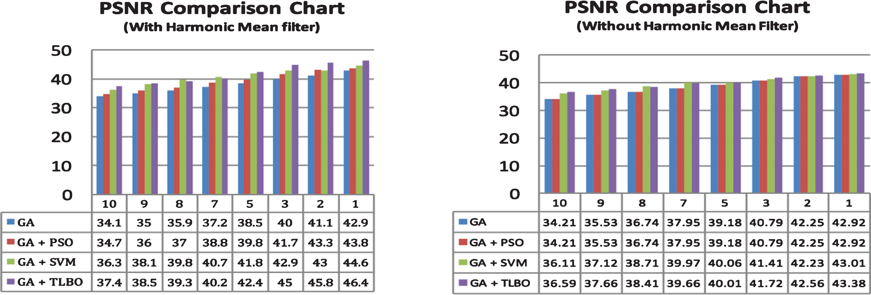
The above graphs represent the PSNR for all the three approaches using PSO, SVM, TLBO alongside with the genetic algorithm through harmonic mean and without harmonic mean. From the above graphs, it is clear that TLBO with GA had exhibited better performance over its counterparts.

Fig.3

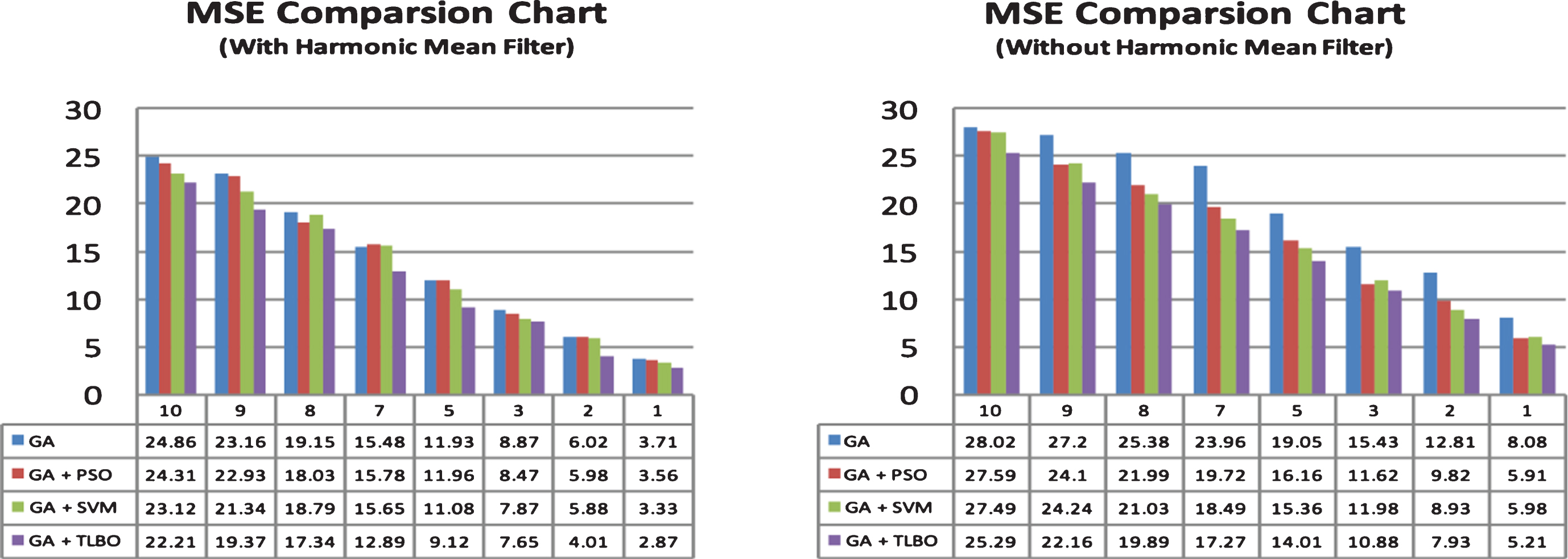
The above graphs represents the MSE for all the three approaches using PSO, SVM, TLBO alongside with the genetic algorithm through harmonic mean and without harmonic mean. From the above graphs, it is clear that TLBO with GA had exhibited better performance and holds the lowest value with the least noise variance value.

From the Tables 1–4 it is understood from the experimental study that the performances of the optimisation techniques seem to be much better when compared to Genetic algorithm alone. Moreover the TLBO based approach has exhbitted a better performances over the other algorithms, where the PSNR and IQI values of TLBO is comparitively high even at significant noise level and MSE, RMSE values are slightly low when compared to that of the other approaches. The values of IQI that are assessed among various approaches are plotted over a graph that can been seen in Figs. 4 and 5.

Table 4

Tabulated values of PSNR, MSE, RMSE, IQI for the segmented image preprocessed through Harmonic mean and without harmonic mean alongside with TLBO over a varied noise

Image Segmentation through harmonic mean and TLBO						Image Segmentation without harmonic mean and with TLBO
S.No	Noise Variance	PSNR Value	MSE Value	RMSE Value	IQI Value	Noise Variance	PSNR Value	MSE Value	RMSE Value	IQI Value
1	10	37.44	22.21	4.83	0.878	10	36.59	25.29	5.02	0.538
2	9	38.52	19.37	4.01	0.971	9	37.66	22.16	4.70	0.572
3	8	39.34	17.34	3.65	0.982	8	38.41	19.89	4.45	0.604
4	7	40.18	12.89	2.98	0.986	7	39.66	17.27	4.15	0.673
5	5	42.35	9.12	1.99	0.989	5	40.01	14.01	3.74	0.723
6	3	44.98	7.65	1.11	0.991	3	41.72	10.88	3.29	0.791
7	2	45.75	4.01	0.97	0.993	2	42.56	7.93	2.83	0.821
8	1	46.38	2.87	0.54	0.996	1	43.38	5.21	2.28	0.879

Fig.4

The above graphs represent the RMSE, which is directly proportional to the MSE for all the three approaches using PSO, SVM, TLBO alongside with the genetic algorithm through the harmonic mean filter. TLBO with GA is proven to be exceptionally better than the other approaches stated above.

Fig.5

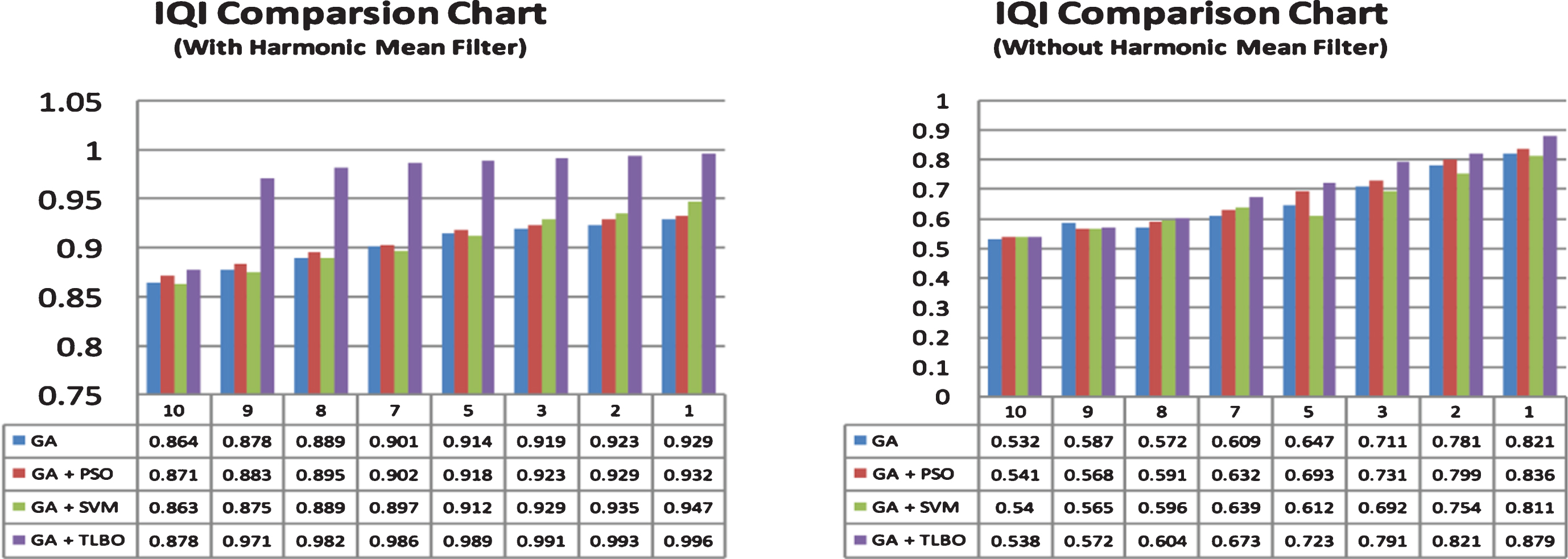
The above graphs represents the image quality index (IQI) for all the three approaches using PSO, SVM, TLBO alongside with the genetic algorithm through harmonic mean and without the harmonic mean filter. The quality of the image through TLBO and the GA nowhere matches with the other approaches.

From Fig. 6 is the graph representing the execution time for the different approaches over an MR image of size 256×256 and 512×512. It is observed from the statistics data in either of the cases the TLBO based approach has taken comparatively marginal time than its counterparts. At times the execution of the PSO based approach and TLBO are identical, but the resultant images of TLBO are more favorable when compared to its counter parts.

Fig.6

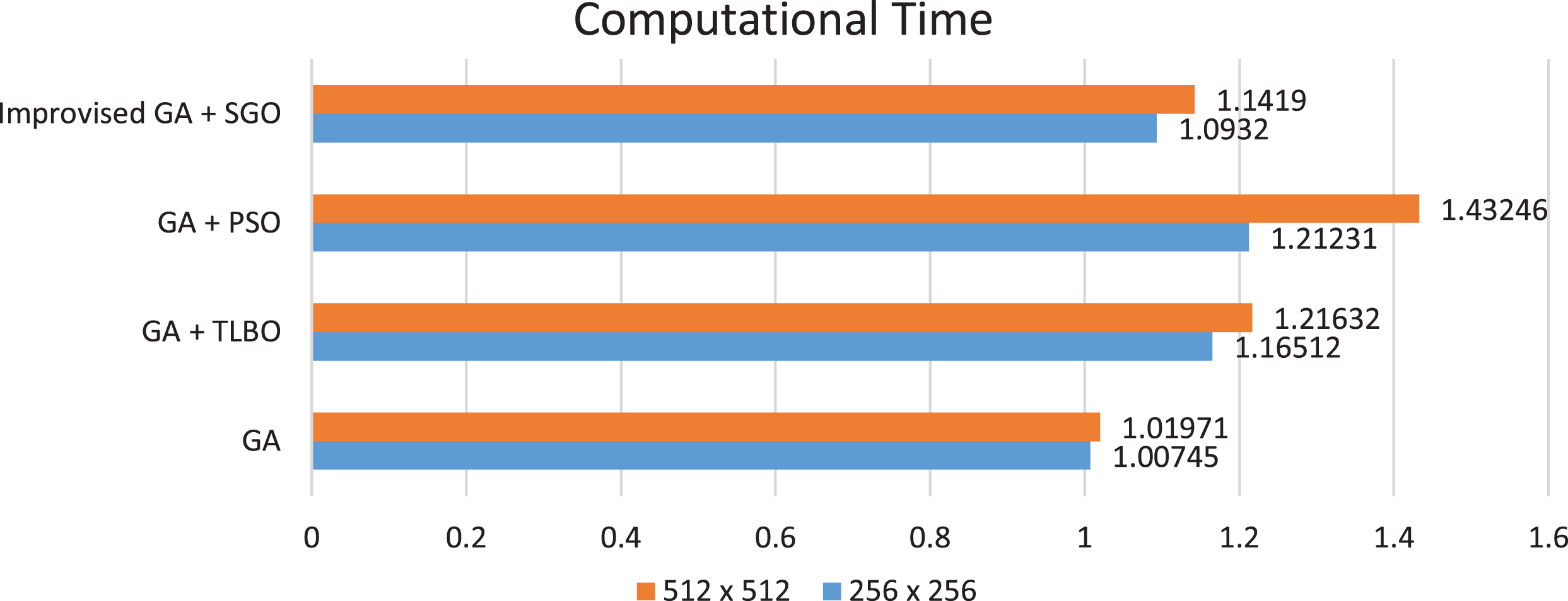
The above bar graph represents the computational time that each algorithm has taken to segment the 256×256 and 512×512 size image with a noise variance of 6. From the above graph, the computational time of GA with TLBO is comparatively low than the PSO and SVM based approach. However, its greater than GA alone but the outcome of GA with TLBO is comparatively better than GA alone.

All the afore mentioned algorithms are implemented over the MR images of size 256×256 and 512×512 with varying noise levels and the computational time for the TLBO is comparatively better the SVM classifier. However, the computation time of TLBO based approach is almost close to the computational time of the PSO algorithm. Still in many cases TLBO has exhibited better performance than its counterpart.

It could be obsereved from the Figs. 7 and 8 that few of the regions in the MR image seems to be having multiple regions in the image MR with identical intensities that would lead to a misinterpritatoin of the damaged region. It could be seen from the afore mentioned figures the SVM based segmented image seems to have multiple smaller regions along with the damaged region and PSO has fiewer and the TLBO based segmentation approach is having an almost negligible number of non-damaged regions higlited when compared to SVM based approach. However, it is advisable to perform skull region removal as stated by P Naga Srinivasu et al. in the article [8] for better identification of the abnormality in the humnan brain through segmentation. The following are the resultant images of the three approaches

Fig.7

The above figure constitutes the segmented image over a noise neutralised input and the color mapped image at divergent intensity levels by which one can easily recognise the effectiveness of the optimisation algorithm in converging towards the automation of lesion identification over iterations.

Fig.8

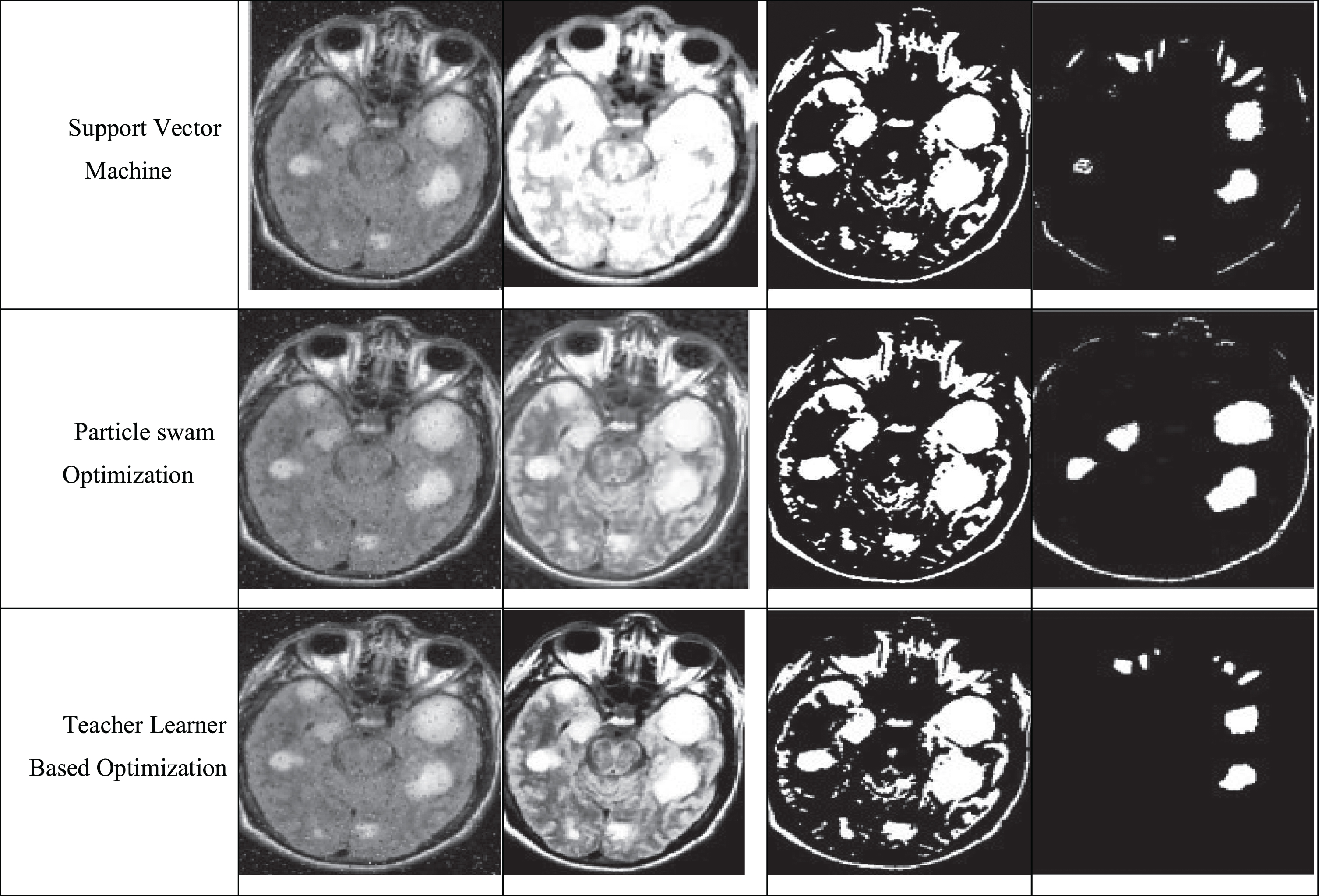
The above figure constitutes the segmented image over a noisy image as input and the color mapped image obtained by segmenting the image. Noise image doesn’t generate the result as good as noise free input.

The performances of the proposed approaches have been assessed through accuracy measuring parametrs like True Positive(TP), True Negative(TN) that designates how many times does a particular algorithm can correctly recognise the damaged region from the segmented image and the algorithm can recognizing the non-tumorous tissues as normal tissues respectively, which is desired to be maximum for a well formulated mechanism. And False Positive(FP) and False Negative(FN), that determines how many times does the specific algorithm fails to correctly recognise the damaged region from the segmented MR image assuming the normal region to be the damaged region and FN determines the number of times does that the algorithm fails in identifying the non-tumoros region as the tumorous region.

The performance evaluation metrics are being implemented over the afore mention approaches that are discussed earlier in this session to evaluate the performances, and the accuracy of all the approaches seems to be nearly the same with minor dissimilarirties. The experimentation that is carried on the images of size 256×256 and 512×512 have been presented in Table 5 below.

Table 5

The above table represents the performance of the various segmentation approaches

	256×256 MR Image				512×512 MR Image
Approaches	TP	TN	FP	FN	TP	TN	FP	FN
GA +PSO	71.29	71.06	28.66	28.68	71.02	70.95	28.69	28.97
GA + SVM	70.61	70.53	29.01	29.26	70.19	70.00	29.88	29.73
GA + TLBO	71.92	71.88	27.97	27.93	71.28	71.21	28.53	28.66

On experimentation, it is observed that the accuracy of the algorithms seems to be identical with minute differences, And all the algorithms have exhbitted better performances of the smaller size image, i.e. MR image of size 256×256 over the MR image of size 512×512. Among all the three experimented approaches, the Teacher Learner Based approach has exhbitted a better performance. However, the computation time for the Genetic Algorithm with Teacher Learner Based optimisations seems to be better than its counter parts, The value of the evaulated metrics are tabulated below in Table 5 for noise normalised images. And the performance of the algorithms over a noise normalised images are much better when compared to that of the experimentation over the noise images. And Fig. 9 is the graph that is generated from the Table 5 where GA with TLBO has exhbitted the better performance.

Fig.9

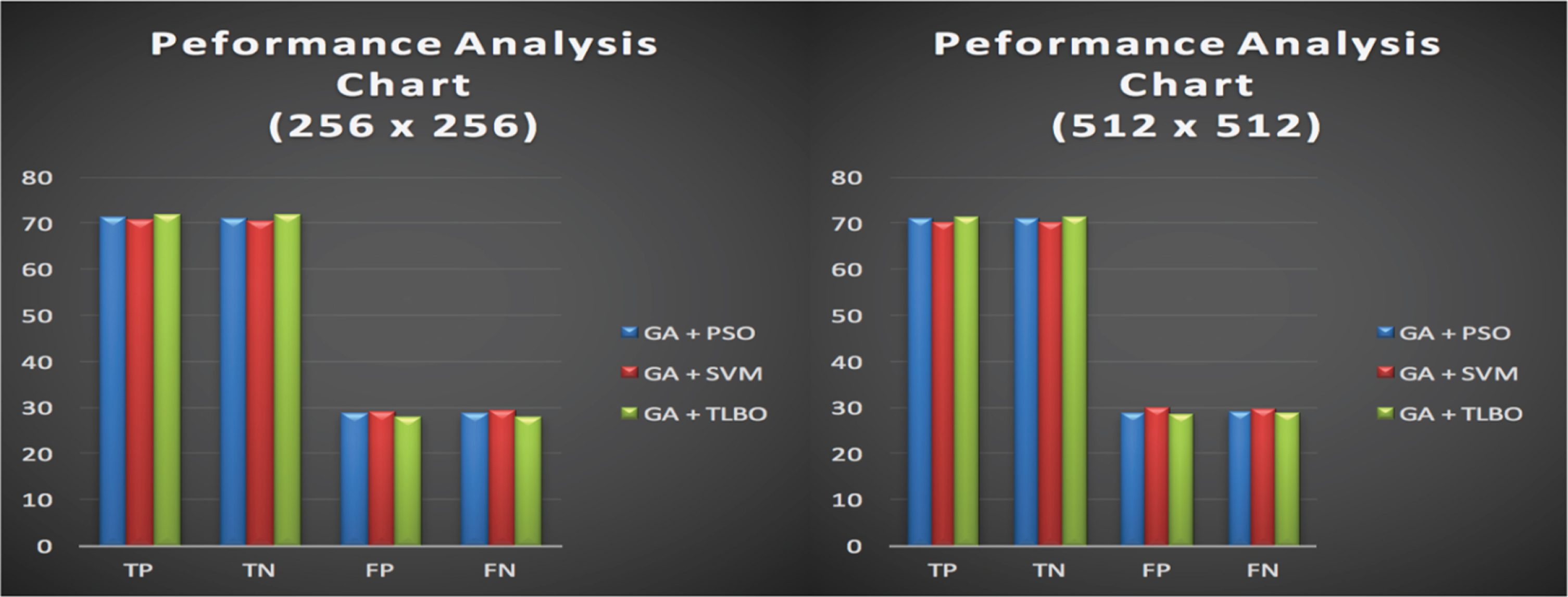
The above bar graphs represents the performances of various approaches over varied size MR Images.

9 Conclusion

In our detailed examination of all the three optimisation techniques PSO, SVM, and TLBO with Genetic Algorithm. It is observed that all three mechanisms work in a better way rather than Genetic algorithm alone. Genetic algorithm with TLBO with an improvised noise reduction strategy has unveiled a divergent result. In few instances with a varied noise impulse over the image, all the three had exhibited an identical performance in tumor detection. And the TLBO based optimisations have conusmed less computational efforts, and it doesn’t have any algorithm specific perameters that helps in ease of converging toward an optimal number of segments.

The working algorithms were evaluated over a wide range of images with varying noise levels and contrast ratio for evaluation of damaged index. The above said mechanisms could be well mechanised by calculating the membership along with the line symmetric based approach for assignment of pixels into the segment. In certain conditions, the borderline pixels or the equidistance pixels may be assigned inappropriately, to circumvent such interpretations the weighted optimisation technique is cooperative. Parameterized TLBO algorithm could address the above said problem in a better way than a standalone approach.

The genetic algorithm supports in estimating the divergent segments that converge to the best possible number of segments. And the optimization techniques would re-arrange the pixles in the segment with respect to the local best segment centroid and the global best centroid. And the stopping criteria must be choosen with at most care for better termination of the algorithm.

10 Future scope

It is observed on the practical implementation of the afore mentioned approach, the Genetic Algorithm itself needs a considerable amount of computational efforts to identify the best possible number of segments and applyimg the optimisation techniques like PSO, SVM and TLBO would obvisouly consume more computational efforts and dignosis latency. It is atmost essential to design an algorithm that could perform better with minimal computatoional efforts. In such scenario it advisable to have a mechnism with enhanced category of the Genetic Algorithm with two point crossover that reduced the time of generating the offspirings, or the entire process of this could also be replaced with multi-objective function based approaches that consumes less computational efforts. It is recommended to mechansie an approach that woould work with all varieties of the medical MR images that include T₁-Weighted, T₂-Weighted and PD weighted MR images.

It is also advised to have a robust pre-processing algorithm that can reduice the noise as well as preserves some of the crucial information related to the objects in the image like edge information and texture based data. In the earlier algorithms only the noise is being addressed that would smoothen the image where some minute regions that are clucial in tumor identification had gone missing. It is advisable to mechanise an approach that can work effieciently over a noise image.

References

Nandi, Detection of human brain tumour using MRI image segmentation and morphological operators, 2015 IEEE International Conference on Computer Graphics, Vision and Information Security (CGVIS), Bhubaneswar, (2015), pp. 55–60.

Khehra

and Pharwaha

A.S.

, Image Segmentation Using Teaching-Learning-Based Optimization Algorithm and Fuzzy Entropy, 15th International Conference on Computational Science and Its Applications, Banff, AB, (2015), pp. 67–71.

Chou

C.-H.

, Hsieh

Y.-Z.

and Su

M.-C.

, A new measure of cluster validity using line symmetry, Journal of Information Science and Engineering30 (2014), 443–461.

Selvaraj

R.D.

, A novel approach for segmentation of brain magnetic resonance imaging using intensity based thresholding, IEEE International Conference on Communication Control and Computing Technologies (2010), pp. 502–507.

Das

and De

, A Modified Genetic Algorithm Based FCM Clustering Algorithm for Magnetic Resonance Image Segmentation. Theory and Applications, Advances in Intelligent Systems and Computing, 515 (2017), Springer, Singapore.

Goshal

, MRI Image Segmentation Using Watershed Transform, IJETAE2(4) (2012).

Mohsen

, Hadhoud

and Mostafa

, A New Image Segmentation Method Based on Particle Swarm Optimization, The International Arab Journal of Information Technology9(5) (2010).

Naga Srinivasu

, Rao

, Srinivas

and Reddy

, A computationally efficient Skull Scraping approach for brain MR Image, Recent Patents on Computer Science (2019), 12. 10.2174/2213275912666190809111928.

Lin

G.-C.

, Multispectral MR images segmentation based on fuzzy knowledge and modified seeded region growing, Magnetic Resonance Imaging. Elsevier30(2) (2013).

10.

Gill

H.S.

, Khehra

B.S.

, Singh

and Kaur

, Teaching-learning-based optimisation algorithm to minimise cross entropy for Selecting multilevel threshold values, Egyptian Informatics Journal (2018).

11.

Lizarazo

, SVM-based segmentation and classification of remotely sensed data, International Journal of Remote Sensing (2008).

12.

Xiao

and Tong

, Research of Brain MRI image segmentation algorithm based on FCM and SVM, The 26th Chinese Control and Decision Conference, Changsha, (2014), pp. 1712–1716.

13.

Teja

K.V.R.

, Rao

N.S.

and Kumar

P.S.

, Distance based algorithm for the removal of salt and pepper noise, 2017 International Conference on Circuit, Power and Computing Technologies (ICCPCT) (2017), pp. 1–5.

14.

Sinha

and Sinha

G.R.

, Efficient Segmentation Methods for Tumor Detection in MRI Images, IEEE Student’s Conference on Electrical Electronics and Computer Science (2014), pp. 1–6.

15.

Benatchba

and Koudil

, Image segmentation using quantum genetic algorithms, IEEE, IECON-2006, France (2007).

16.

Nicoara

, Filip

F.G.

and Paraschiv

, Simulation-based Optimization Using Genetic Algorithms for Multi-objective Flexible JSSP, Studies in Informatics and Control20 (2011), 333–344. 10.24846/v20i4y201101.

17.

EI Zehiry

Noha

, MRI brain extraction using a graph cut based active contour model, IEEE Biomedical Science & Engineering Conference (2009).

18.

Jamil

, Tengku

T.M.

and Bakar

, Noise Removal and Enhancement of Binary Images Using Morphological Operations, IEEE International Symposium on Information Technology (2008), pp. 1–6.

19.

Naga Srinivasu

, Srinivasu

and Srinivas Rao

, An Automated Brain MRI image segmentation using a Generic Algorithm and TLBO, International Journal of Control Theory and Applications9(32) (2016).

20.

Singh

, Bhadauria

H.S.

and Singh

, Automatic brain MRI image segmentation using FCM and LSM, Proceedings of 3rd International Conference on Reliability, Infocom Technologies and Optimization, Noida, (2014), pp. 1–6.

21.

Chen

, Hung

and Zou

, Effective and adaptive algorithm for pepper-and-salt noise removal, IET Image Processing11(9) (2017), 709–716, 9.

22.

Unnikrishnan

, Pantofaru

C.E.

and Hebert

, Toward objective evaluation of Image segmentation algorithms, IEEE Transactions on Pattern Analysis and Machine Intelligence29(6) (2007).

23.

Ait-Aoudia

, Guerrout

and Mahiou

, Medical Image Segmentation Using Particle Swarm Optimization, 18th International Conference on Information Visualisation, Paris, (2014), pp. 287–291. doi: 10.1109/IV.2014.68

24.

Angelina

, Suresh

L.P.

and Veni

S.H.K.

, Image segmentation based on genetic algorithm for region growth and region merging, 2012 International Conference on Computing, Electronics and Electrical Technologies (ICCEET), Kumaracoil, (2012), pp. 970–974.

25.

Saha

, A line symmetry based genetic clustering technique: encoding lines in chromosomes, International Journal of Machine Learning and Cybernetics9(12) (2018), pp. 1963–1986.

26.

Vijendra

and Laxman

, Symmetry Based Automatic Evolution of Clusters: A New Approach to Data Clustering, Computational Intelligence and Neuroscience2015 (2015), Article ID 796276, pp. 21.

27.

Samir

S.R.

and Bandyopadhyay.

, A New Method of Brain Tissues Segmentation from MRI with Accuracy Estimation, Procedia Computer Science85 (2016), 362–369.

28.

Vijay

, Kavitha

A.R.

and Roselene Rebecca

, Automated Brain Tumor Segmentation and Detection in MRI Using Enhanced Darwinian Particle Swarm Optimization (EDPSO), Procedia Computer Science92 (2016), 475–480.

29.

Wang

, Wang

, Zhu

and Meng

, Image segmentation based on Support Vector Machine, Proceedings of 2012 2nd International Conference on Computer Science and Network Technology, Changchun, (2012), pp. 202–206.

30.

Wang

X.-Y.

, Wang

and Bu

, Color image segmentation using pixel wise support vector machine classification. Pattern Recognition, Elsevier. (2010).