Basketball sports neural network model based on nonlinear classification

Abstract

With the continuous innovation of science and technology, the mathematical modeling and analysis of bodily injury in the process of exercise have always been a hot and difficult point in the research field of scholars. Although there are many research results on the nonlinear classification of the basketball sports neural network model, usually only one model is used, which has certain defects. The combination forecasting model based on the ARIMA model and neural network based on LSTM can make up for this defect. In the process of the experiment, the most important is the construction of the combination model and the acquisition of volunteer data in the process of the ball game. In this experiment, the ARIMA model is used as the linear part of the data, and LSTM neural network model is used to get the sequence of body injury. The results of the empirical study show that: it is reasonable to divide the injury of thigh and calf in the process of basketball sports, which is very consistent with the force point of the human body in the process of sports. The results of the two models predicting the average degree of bodily injury for many times are about 0.32 and 0.38 respectively, which are far less than 1. The execution time of the program for simultaneous prediction on the computer is about 1 minute, which is extremely effective.

Keywords

Nonlinear classification neural network radial basis function time-series model basketball

1 Introduction

In recent years, with the development of the economy and the improvement of people’s living standards, many researchers have developed a keen interest in the relationship between physical injuries during exercise and have conducted research on it [1]. How to reduce body damage and consciously reduce energy consumption during exercise? These kinds of motion characteristics are nonlinear and coupled [2] and the human body’s motion parameters will have small changes, which poses a challenge for research. The estimated value can be used as a reference for how people exercise to reduce body damage and provide meaningful help for people to make exercise actions [3].

In this paper, a combination prediction model combining the ARIMA model and LSTM-based neural network is used to predict and collect data such as human body injury caused by thigh and calf movement, and evaluate the model’s prediction accuracy by calculating the standardized mean square error. The relative error of model prediction is about 3%, the prediction value of the model is relatively small, and the prediction accuracy will decrease over time. The relative error of thigh and calf injuries is not very large, indicating that the prediction effect of the BP neural network model has not changed much. The prediction of the BP neural network model is not very good, and the prediction is not very stable [4]. The relative prediction error is 3%. The relative prediction error of the combined model is less than 1%. So we can get that the combined model is more accurate than the single model.

The first chapter of this article is the introduction part, which highlights the importance of this topic from the front according to some domestic and foreign research; the second chapter is the method part, which introduces some knowledge points and techniques used in this article; The third part is the experimental part, which introduces the design and implementation of the performance, and how to collect data; the fourth part is the experimental result analysis part, which analyzes the collected data and compares it with the predicted value to get a conclusion; fifth The chapter is the conclusion part, which is a summary based on the experimental results of this article.

2 Research on basketball sports neural network model based on nonlinear classification

2.1 Related work

Foreign researchers mostly use neural networks to predict body damage, and studying the changes of things over time is the main research content of time series analysis. It can help us discover certain patterns of things and predict the future development of events. We carefully study and carefully observe the characteristics of the time series to discover the hidden laws in the time series [5]. Time series analysis is mainly used to predict the future course of events. Therefore, prediction methods such as neural networks and gray predictions have gradually appeared in our lives and are loved and widely used by everyone. Lingli J proposed the AR model that we are now familiar with [6], and Stout R D proposed the MA model [7]. The most important model used to fit the non-stationary time series is the ARIMA model [8].

Many researchers have made significant contributions to the study of the degree of physical damage caused by exercise and have achieved satisfactory results. Compared with the prediction of the BP neural network using the RBF neural network, the training accuracy and speed of the RBF neural network are obviously better than that of the BP neural network. Once exercise exceeds the limit, the human immune system will be damaged and lose the ability to resist diseases. Excessive or excessive exercise will not only make the body’s metabolism in an extremely intense state. Curtis B and Kaynak proposed four different types of neural networks for determining and comparing the motion parameters of three free athletes [9]; Wang Z proposed neural networks for detecting motion-related nonlinear parameters. The recognition of complex systems has achieved good results [10, 11].

2.2 RBF Neural network

A neural network is a kind of forward neural network with excellent performance, which is suitable for multi-variable and nonlinear operations. As shown in Fig. 1, the more classic is the RBF neural network, which usually includes an input layer, a hidden layer and an output layer. Function approximation is one of the main functions of neural networks. RBF is a local approximation neural network [12, 13]. Once the center is selected correctly, only a few neurons can get the ideal approximation effect.

Fig. 1

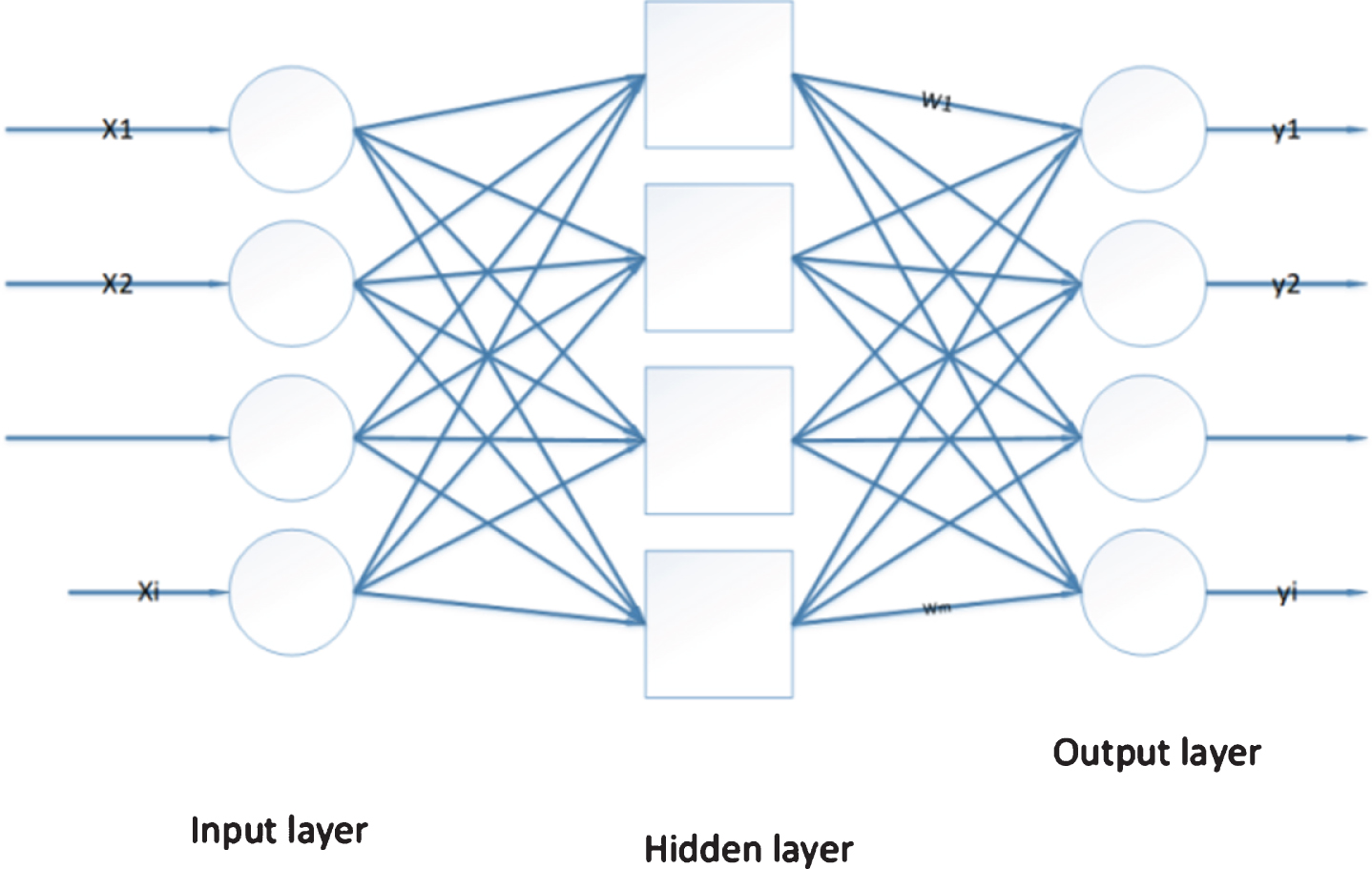
Topology diagram of RBF neural network.

The non-linear mapping function of the RBF neural network has been demonstrated through the function of the hidden layer. Common hidden level basic functions include Gaussian function, thin plate spline function, multiple square functions and inverse multiple square functions, etc. The hidden layer basis function is a standard Gaussian function. $G (| | x - C_{i} | |^{2}) = e^{| | x - C_{i} | |^{2}}$ (1)

In Fig. 1, x_i and y_i are the starting data and the result of the RBF neural network, respectively; ω is the element of the binding weight matrix, and C_i is the core of the Gaussian function.

2.3 Time series model

2.3.1 Characteristic statistics

Average: Accept any time series {Y_t, t ∈ T}, record the distribution function F_t(x) of Y_t, μ_t is the functional expression of the sequence Y_t at t. $μ_{t} = {EY}_{t} = \int_{- \infty}^{\infty} {xdF}_{t} (x)$ (2)

Variance: The degree of fluctuation of the sequence value close to the average is represented by the change function we all know. $D X_{t} = E (X_{t} - μ_{t})^{2} = \int_{- \infty}^{\infty} {(x - μ_{t})}^{2} {dF}_{t} (x)$ (3)

Autocorrelation coefficient: ρ (t, s) is the autocorrelation coefficient of the sequence X_t, abbreviated as ACF.

ρ (t, s) = \frac{γ (t, s)}{\sqrt{{DX}_{t} \cdot {DX}_{s}}}

(4)

When the autocorrelation coefficient is close to 0, the sequence correlation is poor, and when it is close to 1, the sequence correlation is stronger.

2.3.2 Time-series clustering algorithm

Time series data is a set of random data obtained according to time sequence, usually the result of observing a specific process at equal intervals at a given sampling rate. Time series data is real-valued string data, which has the characteristics of large data width, large data volume and continuous data update [14, 15]. Clustering is an unsupervised learning idea, that is, a set of data is divided into different categories according to a specific pattern, and at the same time, the differences between the categories are minimized, and the large differences between the categories are minimized. This article uses the hierarchical clustering method in cluster analysis, which is the most used method in current practice, and it is a method to change the classes from more to less.

The bottom layer of the hierarchical clustering method is: if there are x samples, each sample in the x samples has y attributes, first determine the distance between the samples and the distance between the classes. First, we regard these x samples as x classes, that is, each class contains one sample. Currently, the distance between classes is the same as the distance between samples. Then merge the two closest categories into a new category, and calculate the new category at the same time, and finally merge the distance with other categories according to the minimum distance criterion. According to this process, one category is gradually reduced, and all samples are finally merged into one category. The tree cluster diagram can be used to visually express this combination process. The basic steps for grouping are:

Calculate the distance between every two of these x samples, you can get the distance matrix between samples D⁽⁰⁾;

At the beginning, x samples form a class by itself, that is, the number of classes is k = n, and the t-th class Gt = X(t)(t = 1,2,...,n), which is between classes The distance is the distance between the two samples, and then steps 3) and 4) of the merging process are performed on steps i = 2,...,n;

According to the distance matrix D(i-1) obtained in step i, the two classes with the smallest distance between the merged class and the class are regarded as a new class. At this time, the number of classes k is reduced by 1 class, that is, k = n-i-1;

Measure the distance between the new class and the remaining classes to obtain a new distance matrix D(i). If the total number k of the combined classes is still more than 1, then perform steps 3) and 4) again. Do step 5 until the total number of classes is 1;

Draw a dendrogram;

According to some specific conditions, determine the number of clusters and the samples of each class.

The more classic clustering method is to target static data, that is, data whose characteristics do not change over time, while the characteristics of time series data include data that changes over time, that is, dynamic data. All of them are clustered. When analyzing operations, distance or similar attributes become the key core.

2.4 Neural networks

2.4.1 Fuzzy neural network

Regarding the problem of controlling multiple variables, it is often difficult to confirm the precise mathematical model of the controlled object [16]. Want to get the value of y(k + h|k), so multiple inputs and multiple outputs are used to confirm the fuzzy model. The structure of FNN is divided into four layers [17, 18]. They are the input layer, membership function layer, rule layer and output layer.

(1) The first layer is the input layer. It includes n nodes, each of which is represented as an input variable. The output of this layer is: $u_{i} = x_{i}, i = 1, 2, \dots n$ (5)

Among them, u_i is the output value of the i-th node, and x = [x₁,x₂,...x_n]^T is the input variable.

(2) The second layer is the membership function layer, which includes n*r nodes, each of which is expressed as a membership function of Gaussian function, and the output of this layer is:

$\begin{matrix} μ_{ij} (x_{i}) = & exp [- \frac{(x_{i} - c_{ij})^{2}}{σ_{ij}^{2}}], \\ i = 1, 2, \dots n; j = 1, 2, \dots r \end{matrix}$ (6)

In the function expression, μ_ij represents the jth value of xi, and _cij and σ_ij represent the value of the center and width of the jth of x_i, respectively.

(3) The third layer is the rule layer, which includes r nodes, each of which is represented as the antecedent of a fuzzy rule. The output expression of the j-th rule node is: $φ_{j} (x) = \prod_{i = 1}^{n} μ_{ij} (x_{i}) = exp [- \sum_{i = 1}^{n} \frac{(x_{i} - c_{ij})^{2}}{σ_{ij}^{2}}]$ (7)

Among them, h = [h₁,h₂...,h_t]^T expresses the meaning of the normalized output vector of the rule layer.

(4) The fourth layer is the output layer, which includes many output nodes. The output value of the qth node is the weighted sum of its input data, expressed as L by a functional expression: $y_{q} (x) = \sum_{j = 1}^{r} ω_{jq} h_{j} = \frac{\sum_{j = 1}^{r} ω_{jq} exp [- \sum_{i = 1}^{n} \frac{(x_{i} - c_{ij})^{2}}{σ_{ij}^{2}}]}{\sum_{k = 1}^{r} exp [- \sum_{i = 1}^{n} \frac{(x_{i} - c_{ij})^{2}}{σ_{ik}^{2}}]}$ (8)

Among them, ωjq is the connection weight between the j-th rule node and the q-th output node.

2.4.2 BP neural network

A hierarchical neural network composed of an input layer, middle layer and output layer, the middle layer can be extended to multiple levels. All neurons between adjacent layers can be connected, and all neurons in each layer are completely disconnected. When a pair of learning modes are provided on the network, all neurons will receive network input information and respond at the same time to generate connection weights [19, 20]. Finally, in order to reduce the error value between the expected output result and the actual output result, the output is output from the output layer to the middle layer, and then the middle layer responds back to the input layer, and each layer corrects the connection weight. This process is repeated alternately until the error reported by the global network is close to the minimum value given, that is, the learning process is completed.

The main advantage of the BP neural network is its powerful nonlinear mapping ability. In theory, for a BP network with three or more levels, since the number of hidden level neurons is very large, all the network signals can be close to the nonlinear function with arbitrary precision. At the same time, BP neural network has the ability to connect memory and external stimuli and input information. This is because it uses a method of processing distributed and parallel information, and the extraction of information must use a corresponding method to make all associated neurons operate. The BP neural network uses a pre-stored information learning mechanism for adaptive training, which can recover from the incomplete information state to the initial complete information state. This ability has important technical applications in image restoration, language editing and pattern recognition.

The perceptron network cannot handle the linear inseparability. The emergence of the BP neural network algorithm is a solution to the linear indivisible state. It uses the principle of error propagation to change the traditional network structure, introduce new levels and logic, and fundamentally solve the problem of nonlinear classification. The basic idea of the BP neural network algorithm is: the learning process includes two processes: promotion signal propagation and reverse error propagation. In the forward movement, the input samples pass through the input layer, are processed by the hidden layer, and then passed to the output level. When the output value is very different from the target value, the output error will propagate through the hidden layer in some form, and the error will be distributed to each layer of neurons, and each layer of neurons will use the error signal as a weight modification the basis of [21, 22].

2.4.3 Perceptron neural network

It is a neural network model with only a single layer of neurons, and the function used for network transmission is a linear threshold unit. The first perceptron neural network had only one neuron. It is mainly used to simulate the perceptual characteristics of the human brain [23]. Since the threshold unit is used as a transfer function, only two values can be derived, which is suitable for simple pattern classification problems [24]. When using a perceptron to classify two types of patterns, it is equivalent to separating the two types of samples in a high-dimensional sample space with a hyperplane. However, a single-sided perceptron can only deal with linear problems. The problem is a powerless linear problem.

2.4.4 Linear neural network

A linear neural network is a relatively simple neural network composed of one or more linear neurons. The linear function is used as the transfer function, so the output can have any value. Linear neural networks can use Widrow-Hoff learning rules based on least-squares LMS to change the weights and thresholds of the network [25 –27]. Similar to the perceptron neural network, the linear neural network can only process the linear mapping relationship reflecting the input and output sample space, and it can only be used in linear separability problems.

2.5 Nonlinear and linear classification of neural network

Common linear classifiers are: LR, Bayesian classification, single-layer perceptron, linear regression; common nonlinear classifiers: decision tree, RF, GBDT, multi-layer perceptron SVM.

2.5.1 Yebes classification

Generally, a Bayesian network is a directed acyclic graph. The nodes in the graph represent random variables, which can be observable values, missing variables, positional parameters, or assumptions [27, 28]. The edge generation in the graph represents conditional dependence: unconnected nodes represent that variables are conditionally independent of each other.

The type of random variables represented by Bayesian network nodes can be observable variables or latent variables, unknown parameters, etc [29]. In simple understanding, the arrow arc connecting two nodes means that the two random variables are unconditionally independent or can be regarded as having a causal relationship; and if there are no arrow arcs connected to each other between the nodes, it is said that the random variables are between each other [28 –30]. If two nodes are connected by a single arrow arc, it means that one of the nodes is “Parents” and the other is “Descendants or Children", the two nodes will produce a conditional probability value. The joint probability of the tuple of network variables is calculated by the following formula; $P (y_{1}, \dots, y_{n}) = \prod_{i = 1}^{n} P (y_{i} | pa (Y_{i}))$ (9)

Among them, represents the set of immediate predecessors of Y_i in the network. The value is equal to the value in the conditional probability table associated with Y_i.

For a deterministic Bayesian network, when the value of some variables is given, the inference algorithm can be used to find the value of other target variables [31, 32]. In practical applications, most of the processed variables are random variables, so the exact value of the target variable is generally not assigned. What really needs to be inferred is the probability distribution of the target variable, which means that the target variable is given the observed value of other variables. The probability that the variable takes every possible value [33].

The reasoning method of the Bayesian network is divided into two types: exact reasoning and approximate reasoning. Common precise reasoning algorithms include message passing algorithms, connection tree algorithms, node reduction algorithms, etc.; approximate reasoning algorithms include random sampling algorithms, which are divided into importance sampling methods and Markov chain Monte Carlo methods, as well as search-based algorithms and models, Simplified algorithms, etc., selected from the overview of Bayesian inference algorithms.

2.5.2 Decision tree

A decision tree is a commonly used method in data mining algorithms. It is a method that gradually emerges from the field of machine learning and is used to solve classification functions. The decision tree is a directed acyclic tree result. The bottom layer of the decision tree is the algorithm of classification function approximation. The structure of the decision tree is similar to that of the flowchart, and each of its leaf nodes and child nodes can represent an attribute rule [34].

The decision tree summarizes the learning decision tree from class markers. The decision tree is composed of decision nodes, branches and leaves. Select the most suitable attribute on the root node and all internal nodes to describe it, and then continue to create new branches according to the different values of this attribute. In this way, tree nodes or leaf nodes respectively correspond to a certain class [35, 36]. Use the decision tree algorithm to sort the data, you can visually display the sorting rules.

3 Experimental research on basketball sports neural network model based on nonlinear classification

3.1 Test subject

This research mainly selects 5 team members who have professional knowledge and know that those standard movements are not easy to cause physical damage. This is the experimental group; also 5 amateur basketball enthusiasts who have not received professional training. The movements are not so standard and are more likely to cause body damage. This is the control group. Let the two teams play a basketball game. At the end of each game, all players are tested for body damage and the predicted value is compared to calculate the relative error. Through this experiment, it can be obtained whether the body damage caused by the professional movement is lower than the random movement and compared with the data predicted by the combined model, whether it has higher accuracy and is used for the identification of complex systems and the construction of dynamic systems. Model, real-time prediction and control tool [37].

3.2 Build a combined model

The steps to build the combined model here are as follows:

First, we build an ARIMA model and use the predicted value of the ARIMA model as the linear part of the new combined model.

Build an LSTM neural network model to determine the residual sequence of the ARIMA model. The residual sequence data is input into the LSTM neural network model, and the model output is used as the prediction of the nonlinear part of the body injury sequence after model training.

The data in the two models are added to obtain the predicted body damage prediction value of the combined model.

3.3 Experiment procedure

3.3.1 Build an ARIMA model

The ARIMA model was established based on the data generated by 10 volunteers [38], and the residual sequence length was 10.

3.3.2 LSTM neural network model

To build a network model with only one hidden layer, we set the number of neurons in the three-layer architecture of the LSTM neural network model to 3, 4, and 1. Build a network and get a model. For the residual data generated by 10 volunteers, a table was used to generate 10 training set samples.

3.3.3 Build an improved combination model

The residual sequence obtained by the two models is weighted to obtain the average value, and a new residual sequence is obtained. The neural network is initialized according to the method of LSTM neural network, the residual sequence is nonlinearly predicted, and the nonlinear residual prediction value of body damage is obtained.

3.4 Gather data

In order to verify the feasibility and effectiveness of the entity resolution technology based on the probabilistic soft logic model proposed in this paper, this paper uses the Cora data set and the IMB data set. Cora data set is used as a common entity analysis and evaluation data set. For example, the entity analysis process based on the Markov logic network adopts Cora [39]. This article uses the Cora data set to compare the experimental results with the entity analysis based on the Markov logic network. The IMB data set is not used very frequently in the process of entity analysis experiments, but the IMB data set contains multiple domain entities, as well as multiple entity attributes and ontology information, and is more suitable as an entity analysis experimental data set for multiple data sources.

4 Research and analysis of basketball sports neural network model based on nonlinear classification

4.1 LSTM neural network model predictive analysis

When we call the sim function for network simulation and get the neural network output layer data, we need to denormalize the data to get the body damage prediction value. In order to check the fit of the model [40], we can draw the fitting effect diagram of the model, as shown in Fig. 2.

Fig. 2

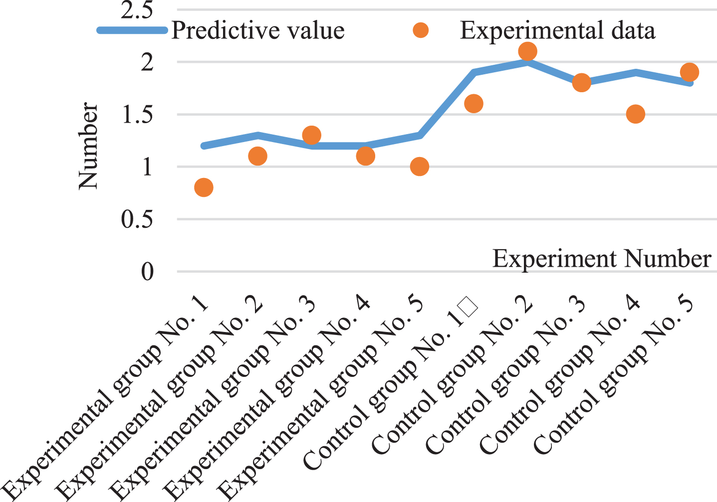
Graph of measured and predicted values of body injury based on LSTM neural network model.

The dots in Fig. 2 represent the real data of 10 volunteers’ body damage scores. From the figure, it can be seen that most of the fitted data is not much different from the real data, and a small part of the data has a relatively large error with the real data. This paper uses the established network model to predict the body injury data of the experimental group and the control group. The predicted value and the actual damage value of the body are compared and analyzed, as shown in Table 1.

Table 1

Experimental group and control group data table

Group	True average	Forecast average	Absolute error	Relative error
Test group	1.06	1.24	0.18	5.07%
Control group	1.78	1.88	0.1	5.33%

From the forecast data in Table 1, it can be seen that the relative error of the model prediction is about 5%, the model prediction value is relatively small, and the prediction accuracy decreases with the increase of the data. The relative error between the two years is not very large, indicating that LSTM The prediction effect of the neural network model does not fluctuate greatly. Of course, overall, the prediction effect of a single LSTM neural network model is not very satisfactory.

4.2 Analysis of body damage based on the combined model

The normalized residual value obtained by the LSTM neural network model is denormalized to obtain the predicted value of the nonlinear part of the sequence [41], which is then added to the predicted value obtained by ARMIA to obtain the combination The final predictive value of the injury score of 10 volunteers of the model. Figure 3 analyzes the predicted value of the combined model and compares it with a single neural network model. The absolute error and relative error are used for model evaluation.

Fig. 3

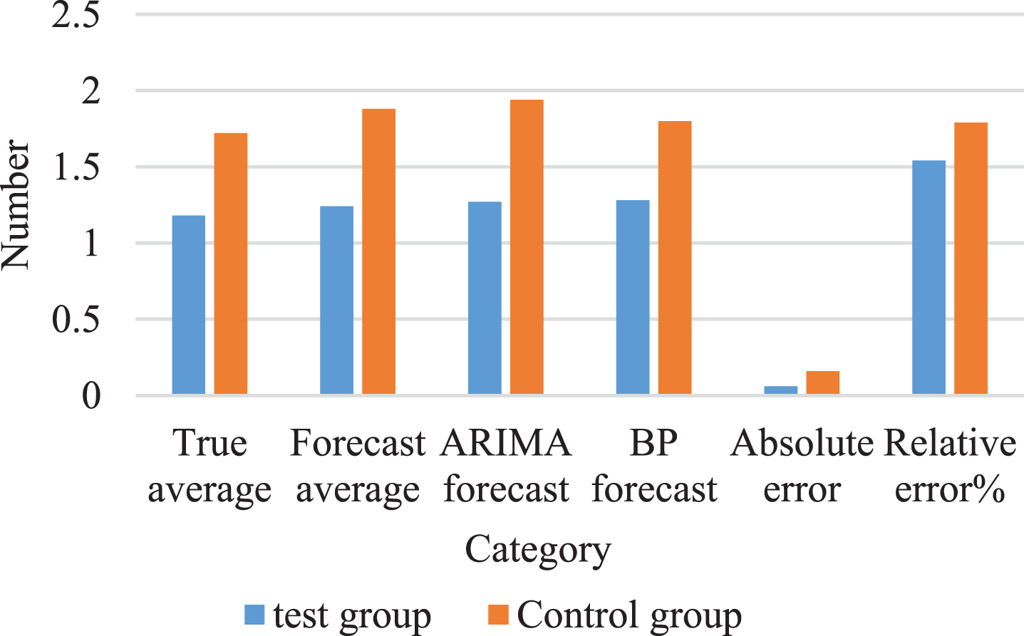
Based on the combination model experimental group and control group data graph.

It can be seen from the data in Fig. 3 that the prediction result of the combined model is lower than the real data, but the prediction effect is better than that of the single LSTM neural network model. Compared with a single LSTM neural network, the relative error of the injury data of the experimental group was reduced by 3.53%, and the relative error of the prediction of the injury data of the control group was also reduced by 3.54%. Therefore, the prediction effect of the model has been significantly improved.

4.3 Model analysis of the improved combination model

4.3.1 Forecast analysis of improved ARIMA model

We decided to use two methods to achieve data stability. One method is to first obtain the logarithm of the data, and then perform the first-order difference to obtain a smooth time series [42]. Another method is to directly run the second-order data difference to obtain a smooth time series. These two methods will eventually obtain a fixed time series. We will create ARMIA models for these two series separately and will receive the predicted values of these two models [43]. These two values are average values, and the result is the linear prediction of the improved combined model, as shown in Fig. 4.

Fig. 4

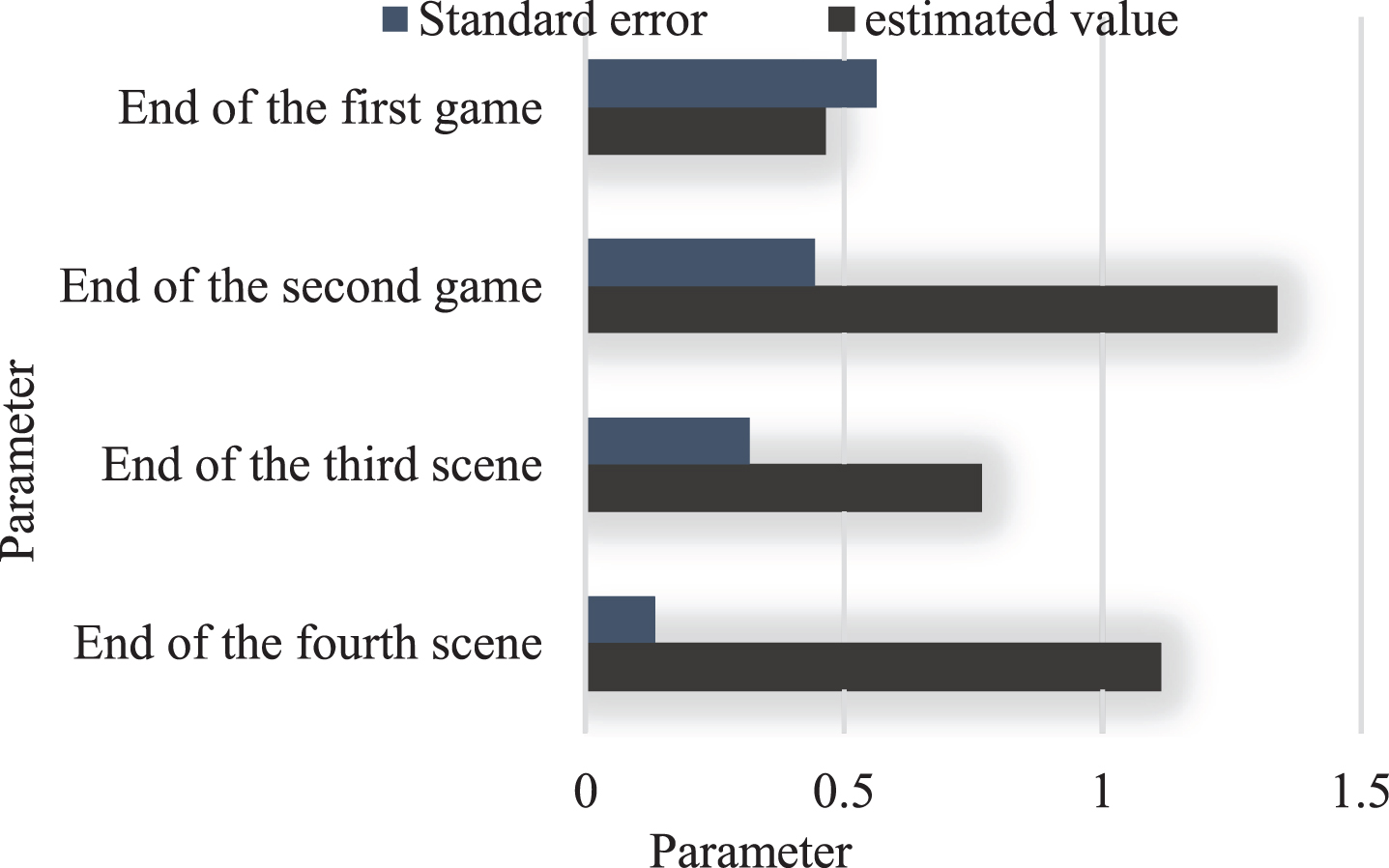
Improved ARIMA model data analysis diagram.

It can be seen from Fig. 4 that the standard error of the ARIMA model predicted value obtained by the second-order difference is smaller and smaller than the true value, while the experimental group’s previous model predicted higher body damage than the true value. The prediction error of the control group is relatively large.

4.3.2 Forecast analysis of improved LSTM neural network model

When using the LSTM neural network for prediction, it is necessary to sample the dominant sequence. Through testing, it is found that when the sample is composed of one input value and one output value, the prediction effect is the best. At the same time, we set the number of LSTM nodes to 4. Under the current settings, the predicted value of body damage is shown in Fig. 5.

Fig. 5

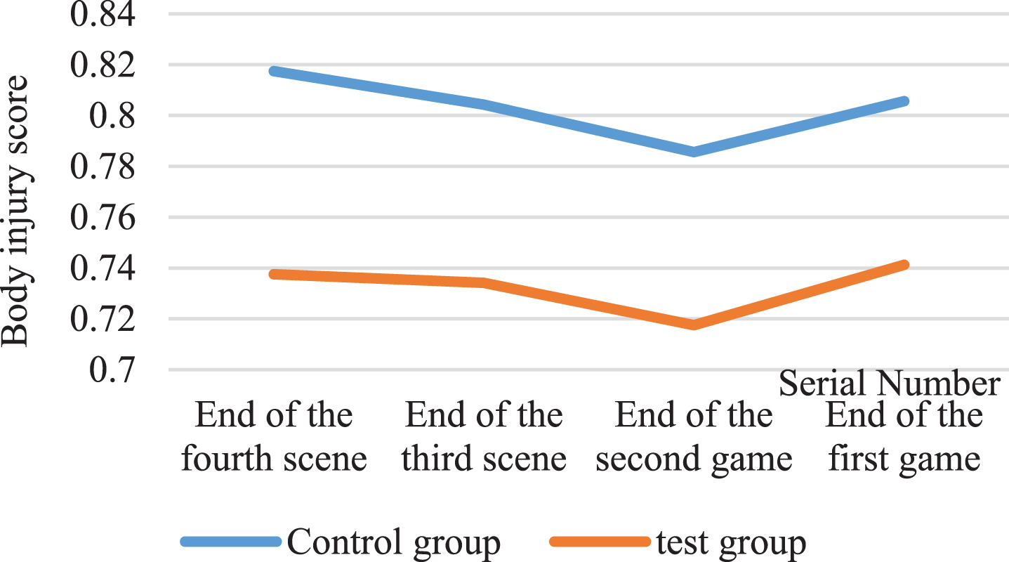
Improved LSTM neural network model prediction data map.

It can be seen from Fig. 5 that the degree of body damage caused by professionally trained people is significantly lower than that of amateurs. At the same time, the body damage and energy consumption of the experimental group were tested in pairs. The standard error level of the mean was 0.262, which was greater than 0.05, indicating that the body damage caused by the experimental group did not have much difference. It also shows that the professionally trained People are less likely to cause damage to their bodies during exercise than amateurs.

5 Conclusions

This article uses a combined prediction model that combines the ARIMA model and the LSTM-based neural network, and predicts the injury and energy consumption of the selected 10 volunteers during and at the end of the exercise, and obtains a better prediction. The accuracy and accuracy of the prediction, at the same time, in terms of operating efficiency, our program runs on the computer for no more than 1 minute, which is very effective in predicting the physical injury of everyone. In the cluster analysis of time series data, this document uses DTW distance as a clustering template. You can also choose other methods as cluster templates, or you can use multiple templates and compare cluster results. When evaluating the accuracy of the model, the average value of NMES is used for comparison, and methods such as AIC and BIC can also be used as standards.

In this article, RBF neural network technology is used to detect various injuries caused by the body during exercise. The collected data is the most input and output data used as RBF sample data, and the RBF neural network is trained with fast running speed and high precision. RBF neural network has a very powerful function approximation ability and extremely outstanding model recognition ability. It can be used in complex system identification, dynamic system modeling and other tools.

In order to make the model prediction more accurate, this paper combines the classic ARIMA model and the LSTM neural network model to form a combined model. The ARIMA model predicts the linear part of various injuries caused by the body during exercise, while the LSTM neural network predicts and estimates the nonlinear balance. Add the data of the two models to get the final predicted value. The combined model is better than the single LSTM neural network model. But compared with the ARIMA model alone, the prediction results are not very satisfactory.

References

Song

and Brandt-Pearce

, Range of Influence and Impact of Physical Impairments in Long-Haul DWDM Systems, in, Journal of Lightwave Technology 31(6) (2013), 846–854.

Shi

, Wang

, Zhong

, Tang

and Cheng

, Hybrid-driven finite-time H ∞ sampling synchronization control for coupling memory complex networks with stochastic cyber attacks, Neurocomputing (Amsterdam) 387 (2020), 241–254.

Zhang

, Qu

, Li

, Luo

and Xu

, A Moving Shadow Elimination Method Based on Fusion of Multi-Feature, IEEE Access 8 (2020), 63971–63982.

Chen

C.-H.

, Song*

, Hwang

F.-J.

and Wu

, A Probability Density Function Generator Based on Neural Networks, Physica A: Statistical Mechanics and its Applications 541 (2020), Article ID 123344.

, Chen*

C.-H.

and Zhang

, A Mobile Positioning Method Based on Deep Learning Techniques, Electronics 8(1) (2019), Article ID 5.

Lingli

, Yilun

, Xuejun

, et al., Degradation Assessment and Fault Diagnosis for Roller Bearing Based on AR Model and Fuzzy Cluster Analysis, Shock & Vibration 18(1-2) (2015), 127–137.

Stout

R.D.

, Jiang

, Matta

, et al., Macrophages Sequentially Change Their Functional Phenotype in Response to Changes in Microenvironmental Influences, Journal of Immunology 175(1) (2005), 342–349.

Arima

, Ginocchio

and Yoshida

, The structure of samarium isotopes in a schematic monopole and quadrupole pairing model, Nuclear Physics A 384(1) (2016), 112–128.

Curtis

, Alanis-Hirsch

, Kaynak

?vgü.

, et al., Using Web searches to track interest in synthetic cannabinoids (aka ‘herbal incense’), Drug & Alcohol Review 34(1) (2015), 105.

10.

Wang

, Li

and Zhang

, Construction waste recycling robot for nails and screws: Computer vision technology and neural network approach, Automation in Construction 97(JAN.) (2019), 220–228.

11.

Wang

, Zhang

X.H.

and Dong

X.C.

, Novel Secure Communication Based on Chaos Synchronization, IEICE Transactions on Fundamentals of Electronics Communications and Computer Sciences E101A, (2018), 1132–1135.

12.

Assareh

and Biglari

, A novel approach to capture the maximum power from variable speed wind turbines using PI controller, RBF neural network and GSA evolutionary algorithm, Renewable & Sustainable Energy Reviews 51(NOV.) (2015), 1023–1037.

13.

Chen

, Shen

, Dai

, et al., Robust Adaptive Sliding-Mode Observer Using RBF Neural Network for Lithium-Ion Battery State of Charge Estimation in Electric Vehicles, IEEE Transactions on Vehicular Technology 65(4) (2016), 1936–1947.

14.

Qin

, Kaile

and Weixiong

, Non-Equal Time Series Clustering Algorithm with Sliding Window STS Distance, Journal of Frontiers of Computer ence & Technology 9(11) (2015), 1301–1313.

15.

Euán

, Ombao

and Ortega

, The Hierarchical Spectral Merger Algorithm A New Time Series Clustering Procedure, Journal of Classification 35(1) (2018), 71–99.

16.

Yin

, Li

, Gao

, Lu

and Zhang

, A Novel Mathematical Model and Multi-Objective Method for the Low-Carbon Flexible Job Shop Scheduling Problem, Sustainable Computing: Informatics and Systems 13(3) (2017), 15–30.

17.

Han

H.-G.

, Ge

L.-M.

and Qiao

J.-F.

, An Adaptive Second-Order Fuzzy Neural Network for Nonlinear System Modeling, Neurocomputing 214(nov.19) (2016), 837–847.

18.

Kim

C.J.

and Chwa

, Obstacle Avoidance Method for Wheeled Mobile Robots Using Interval Type-2 Fuzzy Neural Network, IEEE Transactions on Fuzzy Systems 23(3) (2015), 677–687.

19.

, Wang

, Yan

, et al., Temperature Error Correction Based on BP Neural Network in Meteorological Wireless Sensor Network, International Journal of Sensor Networks 23(4) (2016), 265.

20.

Ren

, Liu

, Yan

, et al., Temperature prediction of the molten salt collector tube using BP neural network, Renewable Power Generation, IET 10(2) (2016), 212–220.

21.

Han

X.H.

, Xiong

and Duan

, A new method for image segmentation based on BP neural network and gravitational search algorithm enhanced by cat chaotic mapping, Applied Intelligence 43(4) (2015), 855–873.

22.

Jing

L.I.

, Weidong

and Fu-Cun

, Simulation of solar radiation in northwest China based on LM-BP neural network, Arid Land Geography 180(2) (2015), 303–313.

23.

Moallem

, Abdollahi

M.A.

and Hashemi

, Compensation of Capacitive Differential Pressure Sensor using Multi-Layer Perceptron Neural Network, International Journal on Smart Sensing and Intelligent Systems 8(3) (2015), 1443–1463.

24.

Liu

, Yang

and Sun

, Thresholds Based Image Extraction Schemes in Big Data Environment in Intelligent Traffic Management, IEEE Transactions on Intelligent Transportation Systems (2020), 1–9.

25.

Egrioglu

, Yolcu

, Aladag

C.H.

, et al., Recurrent Multiplicative Neuron Model Artificial Neural Network for Non-linear Time Series Forecasting, Neural Processing Letters 41(2) (2015), 249–258.

26.

Yin

, Shen

, Liu

, et al., Simultaneous quantitative UV spectrophotometric determination of multicomponent of amino acids using linear neural network, Computers & Chemistry 25(3) (2001), 239–243.

27.

Bangzhu

, Shunxin

and Minxing

, Achieving the Carbon Intensity Target of China: A Least Squares Support Vector Machine with Mixture Kernel Function Approach, Applied Energy 233 (2019), 196–207.

28.

, Khan

and Garaniya

, Modified independent component analysis and Bayesian network-based two-stage fault diagnosis of process operations, Industrial & Engineering Chemistry Research 54(10) (2015), 1–19.

29.

and Yang

, Modeling and analysis of cascading node-link failures in multi-sink wireless sensor networks, Reliability Engineering & System Safety 197 (2020), 106815.

30.

J.G.

, Zhao

, Chen

, et al., A Structure Learning Algorithm for Bayesian Network Using Prior Knowledge, Journal of Computer ence and Technology 30(4) (2015), 713–724.

31.

Tschiatschek

and Pernkopf

, On Bayesian Network Classifiers with Reduced Precision Parameters, IEEE Transactions on Pattern Analysis & Machine Intelligence 37(4) (2015), 774–785.

32.

Gutierrez

B.T.

, Plant

N.G.

, Thieler

E.R.

, et al., Using a Bayesian network to predict barrier island geomorphologic characteristics, Journal of Geophysical Research Earth Surface 120(12) (2015), 2452–2475.

33.

, Zhao

and Xiong

, Cross-layer congestion control of wireless sensor networks based on fuzzy sliding mode control, Neural Computing and Applications. (2020).

34.

Samantaray

S.R.

, Decision tree-based fault zone identification and fault classification in flexible AC transmissions-based transmission line, Iet Generation Transmission & Distribution 3(5) (2015), 1–6.

35.

Wang

, Fan

, Hsu

C.H.

, et al., A Vertical Handoff Method via Self-Selection Decision Tree for the Internet of Vehicles, IEEE Systems Journal 10(3) (2016), 1183–1192.

36.

Zhang

and Suganthan

P.N.

, Oblique Decision Tree Ensemble via Multisurface Proximal Support Vector Machine, IEEE Transactions on Cybernetics 45(10) (2015), 2165–2176.

37.

Zeng

H.-B.

, Teo

K.L.

, He

and Wang

, Sampled-data-based dissipative control of T-S fuzzy systems, Applied Mathematical Modelling 65 (2019), 415–427.

38.

Singh

and Agrawal

, A Customer Centric Best Connected Channel Model for Heterogeneous and Iot Networks, Journal of Organizational and End User Computing 30(4) (2018), 32–50.

39.

Xiao

, Cheng

and Zhang

, Detecting travel modes from smartphone-based travel surveys with continuous hidden Markov models, International Journal of Distributed Sensor Networks 15(4) (2019), 1–15.

40.

, Xiong

, Chen

, Cao

, Huang

, Yang...

and Chen

, Image quality enhanced recognition of laser cavity based on improved random hough transform, Journal of Visual Communication and Image Representation (2019), 102679.

41.

Tharwat

, Mahdi

, Elhoseny

and Hassanien

A.E.

, Recognizing human activity in mobile crowdsensing environment using an optimized k-NN algorithm, Expert Systems with Applications 107 (2018), 32–44.

42.

Sun

, Yang

and Xu

, Adaptive differential evolution with a combined strategy for global numerical optimization, Soft Computing 24(9) (2020), 6277–6296.

43.

Quan

, Zou

, Huang

and Lei

, Research on water temperature prediction based on improved support vector regression, Neural Computing & Applications (2020).