Logistics demand forecasting model based on improved neural network algorithm

Abstract

The irrationality between the procurement and distribution of the logistics system increases unnecessary circulation links and greatly reduces logistics efficiency, which not only causes a waste of transportation resources, but also increases logistics costs. In order to improve the operation efficiency of the logistics system, based on the improved neural network algorithm, this paper combines the logistic regression algorithm to construct a logistics demand forecasting model based on the improved neural network algorithm. Moreover, according to the characteristics of the complexity of the data in the data mining task itself, this article optimizes the ladder network structure, and combines its supervisory decision-making part with the shallow network to make the model more suitable for logistics demand forecasting. In addition, this paper analyzes the performance of the model based on examples and uses the grey relational analysis method to give the degree of correlation between each influencing factor and logistics demand. The research results show that the model constructed in this paper is reasonable and can be analyzed from a practical perspective.

Keywords

Neural network improved algorithm logistics demand forecasting model

1 Introduction

Logistics demand is the product of economic activity behavior, which refers to the demand generated when economic activity behavior configures resources in a certain period of time, and involves every link of logistics activity. This demand is not only reflected in time and space, but also in higher requirements for quantity and quality. Moreover, this demand runs through the entire logistics process. The diversified and rapidly developing social economy has broadened the development space of the logistics industry and promoted the diversified and complex development of the logistics industry. In this context, the decision-making and planning of the logistics industry is particularly important to the development of the logistics industry. Moreover, accurate forecasting of logistics demand can provide a scientific basis for decision-makers’ decisions and play an important role in the development of the logistics industry. However, accurate logistics demand forecasting requires a more solid theoretical and scientific basis [1].

Whether the choice of the forecasting model is reasonable or not will affect the forecasting accuracy to a large extent. To obtain high-precision prediction simulation results, it is necessary to select a reasonable prediction model. It is necessary to analyze the characteristics of statistical data, and select a model method that is most suitable and easy to implement according to the data characteristics obtained by the analysis, so as to obtain higher precision and scientific and reasonable prediction results. Sometimes, the effective combination of multiple models can effectively make up for the shortcomings of a single model, obtain higher prediction accuracy than a single model, and obtain more reasonable and accurate prediction results. Therefore, building a combined forecasting model is also an important idea when building a forecasting model [2].

The logistics involves a series of processes in social economic activities from the initial demand, supply, production, product circulation to consumption. The logistics demand is the demand generated when resources are allocated in these processes. Therefore, logistics demand is a product of social economic activities, but also an important part of it. This article mainly analyzes the factors that can quantitatively measure the influence of logistics demand from five aspects: regional GDP, industrial structure, resident consumption level, domestic and foreign trade, and logistics infrastructure construction.

Cargo turnover includes two aspects: the quantity and distance of the transported goods, which can fully reflect the production results of the transport of goods. The logistics demand for transportation is only one part of the logistics demand and cannot fully reflect the logistics demand. However, cargo transportation volume and freight turnover volume account for a large proportion of the logistics volume, which can reflect the changing law of logistics demand and the total logistics demand in a specific area to a certain extent [3].

2 Related work

When studying the forecast of the demand for cold chain logistics of agricultural products, the literature [4] analyzed the current situation and existing problems of cold chain logistics of agricultural products, and then used the cold chain logistics to predict and put forward corresponding countermeasures. The literature [5] pointed out that the simple cargo transportation volume is enough to describe the logistics demand, and proposed that the logistics demand should be converted by the cargo transportation volume and the cargo volume in other links of logistics activities. The literature [6] used the total amount of agricultural product logistics as an index to measure agricultural product logistics demand, and analyzed and selected the influencing factors of agricultural product logistics demand from two aspects: agricultural product output and external economic environment. The literature [7] used the BP neural network prediction method to predict the logistics demand of agricultural products, and used the total logistics of agricultural products to measure the logistics demand of agricultural products, and also proposed an algorithm for the total logistics of agricultural products. The literature [8] analyzed the relationship between regional economic factors and regional logistics demand, and constructed an SVR prediction model for prediction research. The literature [9] used the correlation analysis method to analyze the factors that affect the level of logistics development in Fuzhou, and found out GDP, industrial output value, total import and export volume, and total retail sales of consumer goods and other economic indicators that have a greater correlation with the level of logistics development. The literature [10] believed that the very important prerequisite for urban logistics planning is to first make a scientific and accurate forecast of urban logistics demand, and built a multi-population genetic BP neural network model to forecast logistics demand. The literature [11] pointed out that when forecasting logistics demand, not only the influence of economic factors must be considered, but also industry factors such as logistics facilities and logistics services. Moreover, it also proposed a combined model that combines Grey Relational Analysis (GRA) and Least Squares Support Vector Machine (LSSVM). This combination model first uses grey relational analysis to screen the main influencing factors of logistics demand, and predicts the selected influencing factors as input variables of the LSSVM model. The literature [12] optimized the model, and used the kernel principal component analysis (KPCA) to eliminate the multiple correlations between the main influencing factors screened by GRA, and used the improved particle swarm optimization (IPSO) algorithm to optimize and adjust the parameters of the LSSVM model. At the same time, in the analysis of influencing factors, factors such as price level, population size and logistics information technology are analyzed.

The literature [13] pointed out that seasonal changes in certain regions would have a huge impact on local logistics demand, and based on this, created a combined forecasting model based on seasonal index and gray GM (1, 1). Moreover, it demonstrated the validity and feasibility of the model. The literature [14] combined linear regression with DGM (1, 1) model to propose a combined model based on the two, and conducted an empirical analysis of logistics demand. The results show that the DGM (1,1) model has the best prediction effect when the requirements for prediction accuracy are high and the data samples are small. The literature [15] constructed a gray GM (1,1) linear combination prediction model. After that, it applied the ant colony algorithm to the gray linear combination model, optimized the weights of the individual models in the combination model, and established a GM (1, 1) linear combination model based on the improvement of the ant colony algorithm. The results show that the improved grey linear combination forecasting model has a better fitting effect, and the forecasting accuracy is higher than the other two forecasting methods. The literature [16] proposed a method for forecasting logistics demand based on an input-output economic model, which to a certain extent provides a theoretical reference for logistics development planning. The literature [17] pointed out that logistics demand is closely related to the level of economic development, and constructed three models: gray prediction model, neural network model and gray neural network combination model. Moreover, it used genetic algorithm (GA) to optimize and improve the three models respectively, and constructs GA-GM (1,1). The literature [18] used the artificial fish school algorithm (AFSA) to optimize the parameters of the support vector machine (SVM) to propose an AFSA-SVM combination forecasting model of logistics demand. The literature [19] constructed an optimized combination prediction model based on dynamic adaptive particle swarm optimization algorithm (DAPSO) and unbiased grey prediction model (UGM (1,1)). The prediction results show the effective feasibility of the combination model. The literature [20] combined the GM (1, N) model with the BP neural network model to establish a gray neural network model, and based on this, developed a logistics demand forecasting system. The results show that the gray neural network combination model can effectively predict short-term logistics demand, and has higher prediction accuracy of a single model, which proves the effectiveness of the combination model.

3 Logistic regression algorithm

The principle of logistic regression is similar to that of linear regression. Logistic regression also requires a weighted sum of data features. However, unlike linear regression directly outputting the weighted sum, the logistic regression algorithm needs to calculate the weighted sum through the sigmoid function and output it. The mathematical expression of using logistic regression to predict probability is shown in formula (1) [21]. $\hat{p} = h_{θ} (x) = σ (θ^{T} x)$ (1)

Function σ (·) is a sigmoid function, which can map data between 0 and 1. The specific mathematical form is shown in formula (2): $σ (t) = \frac{1}{1 + exp (- t)}$ (2)

After the logistic regression model predicts the probability $\hat{p}$ of the sample x, the type of sample can be judged by formula (3): $\hat{y} = {\begin{matrix} 0 & if \hat{p} < 0.5 \\ 1 & if \hat{p} ⩾ 0.5 \end{matrix}$ (3)

The logistic regression model predicts and classifies the probability of a sample through the above steps. Next, we discuss the training steps of the model. According to the practical significance of the model, the training target of the model can be easily seen. For samples with label 1, the predicted probability needs to be as large as possible. For samples with a label of 0, the predicted probability needs to be as small as possible. This idea can be described by formula (4), and the loss function of a single sample is given [22]. $c (θ) = {\begin{matrix} - log (\hat{p}) & if y = 1 \\ - log (1 - \hat{p}) & if y = 0 \end{matrix}$ (4)

It can be seen from the error function of a single sample that when $\hat{p}$ tends to 0, the value of $- log (\hat{p})$ tends to positive infinity. This means that when the predicted probability of a positive sample tends to zero, the loss of the sample will be large. Similarly, when the predicted probability of a sample with 0 label is close to 1, the loss function will also become larger. On the other hand, when the model correctly predicts the sample label, the loss will tend to 0, which is exactly what we want the model to achieve.

The loss function of the entire training set can be written as the average loss of all samples. The specific form is shown in formula (5):

$\begin{matrix} J (θ) = & - \frac{1}{m} \sum_{i = 1}^{m} [y_{i} log ({\hat{p}}_{i}) \\ + (1 - y_{i}) log (1 - log ({\hat{p}}_{i}))] \end{matrix}$ (5)

By solving the minimum value of the loss function, the parameter set θ is determined. However, there is no way to find the closed solution of the loss function equation. However, because the loss function is a convex function, the global optimal solution of the function can be obtained through the gradient descent algorithm. The gradient descent algorithm only needs to calculate the partial differential of the loss function. The specific form of solving the j-th dimension gradient is shown in formula (6) [23]: $\frac{\partial}{\partial θ_{j}} J (θ) = \frac{1}{m} \sum_{i = 1}^{m} (σ (θ^{T} \cdot x^{(i)}) - y^{(i)}) x_{j}^{(i)}$ (6)

4 Common regular terms of logistic regression algorithm

In order to prevent the logistic regression algorithm from overfitting when building the model, some regular terms are usually added to the cost function. The occurrence of over-fitting is usually caused by excessively high model parameters. The purpose of adding regular items is to limit the parameters. Common regularization methods are L₁ and L₂ regularization. For linear regression models, the model using L₁ regularization is called Lasso regression, and the model using L₂ regularization is called Ridge regression.

Lasso regression adds the L₁ norm of the weight to the original loss function J₀ as the penalty term of the loss function. The final form of the objective function is shown in formula (7): $J = J_{0} + α \sum_{i}^{n} | W_{i} |$ (7)

When using L₁ regularization, due to the nature of the L₁ norm, the weights of features with lower importance will tend to zero. Therefore, L₁ regularization also plays a role in feature selection. The process of solving the cost function is shown in Fig. 1. The contour of the graph is the contour of J₀, and the black square is the graph of L₁ norm. In the figure, the first intersection of the J₀ contour and the L₁ graph is the optimal solution. J₀ and L₁ intersect at a vertex, and this vertex is the optimal solution.

Fig. 1

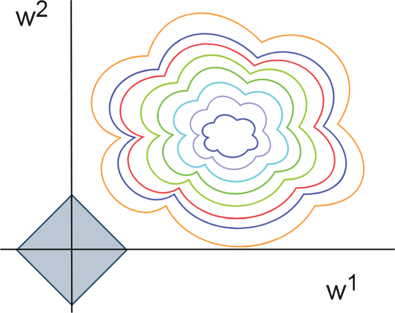
The solution of the cost function with L₁ regular term.

The probability of J₀ contacting these vertices is much greater than the probability of contacting other parts of the L₁ norm. However, in these corners, there will be many weights equal to zero. Then, there will be more features of 0 in the multi-dimensional features. This is why L₁ regularization can produce sparse models, which can then be used for feature selection [24].

The regular term of Ridge regression is the L₂ norm of the weights, and the specific form of the objective function is shown in formula (8): $J = J_{0} + \frac{α}{2} \sum_{i}^{n} W_{i}^{2}$ (8)

L₂ regularization usually makes the final feature weight of the model smaller, so as to prevent the model from overfitting. The magnitude of model regularization is adjusted by adjusting parameter α. The increase of α will increase the generalization ability of the model, but at the same time reduce the expressive ability of the model. In practical applications, the appropriate parameter α can be selected through model performance. The process of solving the cost function is shown in Fig. 2. The contour of the graph is the contour of J₀, and the black circle is the graph of L₂ norm. In the figure, the first intersection of the J₀ contour and the L₂ figure is the optimal solution. This intersection is the optimal solution. The graph of L₂ norm in the two-dimensional plane is a circle. Compared with the square, its edges and corners have been removed. Therefore, the intersection of J₀ and L₂ makes the probability of the weight equal to zero much smaller. This is why L₂ regularization is not sparsity.

Fig. 2

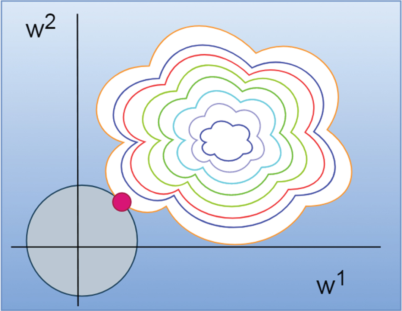
The solution of the cost function with L₂ regular term.

Another form of regular term is a mixed form of L₁ norm and L₂ norm. The specific form of the objective function is shown in formula (9): $J = J_{0} + r α \sum_{i}^{n} | W_{i} | + \frac{(1 - r)}{2} α \sum_{i}^{n} W_{i}^{2}$ (9)

This regular term can control the mixing degree of L₁ norm and L₂ norm by adjusting the ratio r. When r = 1, its cost function form is the same as Lasso regression. When r = 0, the cost function form is the same as Ridge regression [25].

The algorithm model of the automatic encoder is also built around this purpose, and the specific structure is shown in Fig. 3. The auto-encoder learns the characteristic representation of the data by encoding the network, which can also be understood as the pattern of the data. Then, it restores the original data through the decoding network.

Fig. 3

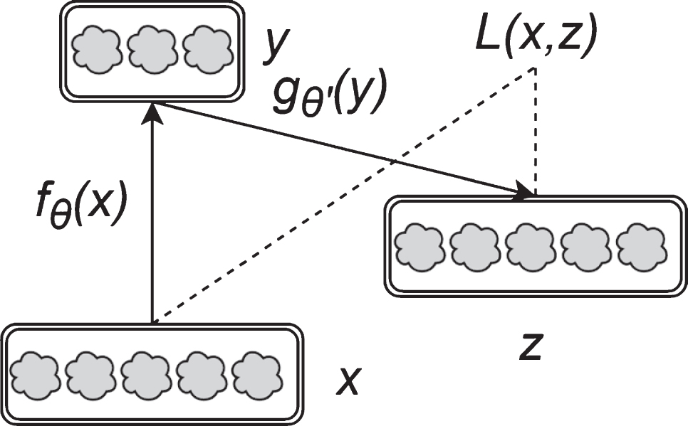
Single-layer automatic encoder structure diagram.

Now, we assume that there is a series of unlabeled samples {x⁽¹⁾, x⁽²⁾, x⁽³⁾, ⋯ , x^(N) }, and the sample x is a d-dimensional vector $x \in ℝ^{d}$ . A more abstract feature indicates that y needs to be extracted from the original data, y is a d′-dimensional vector, $y \in ℝ^{d^{'}}$ .

The encoder part maps the data x into an abstract feature representation y, and f_θ (x) is the mapping function, as shown in formula (10). The parameter set is θ = { W, b }, W is the d′ × d-dimensional weight matrix, and b is the d′-dimensional offset vector. $f_{θ} (x) = s {Wx + b}$ (10)

s is usually a nonlinear activation function, and sigmod activation function is often used.

The decoder part reconstructs the original input data x from the abstract feature representation y, generates a reconstruction vector z, and makes the reconstructed data as close to the original input data as possible. Among them, z = g_θ (y), g_θ are the mapping functions of the decoding part, as shown in formula (11). $g_{θ^{'}} (y) = s {W^{'} y + b^{'}}$ (11)

The parameter set is θ′ = { W′, b′ }. If the input sample is not only in the interval [0, 1], it is more in line with our perception not to use the nonlinear function s. L (x, z) is the reconstruction error of the autoencoder, which is used to represent the difference between the reconstructed signal and the input signal. The measurement of the difference is also often related to the distribution of the input data x.

For the real vector x, that is $x \in ℝ^{d}$ . The input data often obey the normal distribution, and the form of the loss function L (x, z) is often used in the form of formula (12). For normally distributed data, the sum of square error is often more commonly used, and C is a constant. $L (x, z) = \sum C | x - z |^{2}$ (12)

If the input data is x ∈ [0, 1] ^d, the reconstructed vector output by the decoder must be in the same interval as the input data. The decoder also usually uses the non-linear function sigmod activation function to achieve this goal. In this case, the cross entropy function is usually used. The form of loss function L (x, z) is shown in formula (13). $L (x, z) = - \sum_{j} x_{j} log z_{j} + (1 - x_{j}) log (1 - z_{j})$ (13)

The autoencoder trains the model by minimizing the reconstruction error L (x, z), so that the reconstructed signal still retains most of the information of the input signal. Moreover, it determines the parameter set {θ, θ′} by solving the minimum value of the loss function, thereby obtaining the encoder function and the decoder function. The optimization function is shown in formula (14). $arg min_{θ, θ^{'}} L (x, z)$ (14)

If the non-linear activation function is not used in the encoder and decoder functions, its form is almost the same as that of PCA (Principal Component Analysis). The functional form that minimizes the reconstruction error is the same as the functional form that maximizes the lower bound of the mutual information between the input signal x and the hidden layer feature representation y. It can be seen that the autoencoder extracts abstract features by maximizing the information of the input data.

5 Ladder network

The ladder network structure is shown in Fig. 4, including a forward neural network for output and a decoding network for reconstructing each layer. x represents the input data, $\tilde{x}$ represents the data after adding noise, and $\hat{x}$ represents the reconstructed input data. Meanwhile, z^(l) represents the hidden variable of each layer. Similarly, ${\tilde{z}}^{(l)}$ represents the hidden variable adding noise, and ${\hat{z}}^{(l)}$ represents the hidden variable after reconstruction. The forward path is x → z⁽¹⁾ → z⁽²⁾ → y, the noise-adding path is $x \to {\tilde{z}}^{(1)} \to {\tilde{z}}^{(2)} \to \tilde{y}$ , and the coding functions share the same f^(l). At the same time, the decoding path is ${\tilde{z}}^{(l)} \to \hat{z} \to \hat{x}$ and the decoding function is $g^{(l)} ({\tilde{z}}^{(l)}, {\hat{z}}^{(l + 1)})$ , which is different from the decoding function of DAE. The ladder network adds the same layer connection from the encoder to the decoder. The unsupervised loss function of each layer is $C_{d}^{l}$ . Since the activation function of each layer uses the relu activation function, the specific form of the loss function is $| \hat{z} - z |^{2}$ . The ladder network solves the parameters of the encoding and decoding functions through training, and finally outputs the final result through the un-noise-adding path.

Fig. 4

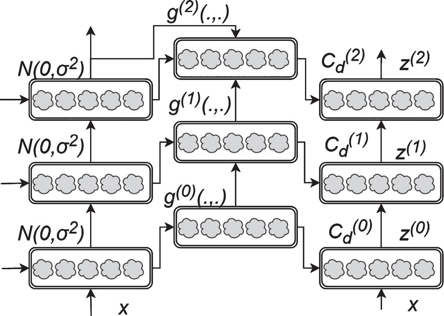
Ladder network structure.

In the case of unlabeled data, the ladder network can also effectively improve the performance of the model by purely supervised learning training. The general implementation steps are as follows:

First a suitable encoder network is selected. The type of network is not limited to the traditional multilayer perceptron model. For different tasks, convolutional network (CNN) or recurrent neural network (RNN) can be selected as the coding network.

For each layer of hidden variables, we analyze its conditional distribution p (z^(l)|z^(l+1)) to the upper layer of hidden variables. For different distributions, the form is also different.

Then, the decoding function $g^{(l)} ({\tilde{z}}^{(l)}, {\hat{z}}^{(l + 1)})$ is determined, so that it can effectively estimate the current distribution. The decoding function determines the reconstruction hidden variables of this layer by combining the reconstruction hidden variables of the previous layer and the noise-adding hidden variables of the same layer.

Finally, the entire network is trained through supervised learning or semi-supervised learning. The optimization algorithm can choose stochastic gradient descent or Adam algorithm.

The specific algorithm for batch standardization operation for the first layer is as follows: $BN (x) = \frac{x - μ_{x}}{σ_{x}}$ (15) $z^{(l)} = BN (W^{(l)} h^{(l - 1)})$ (16) $h^{(l)} = φ (r^{(l)} (z^{(l)} + β^{(l)}))$ (17)

The batch function BN will perform the operation as in formula (6) on each x vector. μ_x is the mean value of the small batch data, and σ_x is the corresponding standard deviation. The mean and standard deviation will be estimated from the mini-batch used for training. For the initial value h⁽⁰⁾, the initial value is such that h⁽⁰⁾ = x, r^(l) and β^(l) will be set as the expansion factor and bias factor of the activation function of each layer. They are all trainable parameters. φ (·) is the activation function of each layer of the network. For some activation functions, the expansion factor will be redundant and can be omitted when building the model, such as the relu function φ (·) = max(0, ·). For linear activation functions, both the stretch parameter and the bias parameter can be omitted. However, for the softmax function, both are often indispensable.

The ladder network requires two forward processes to find the output of noise-adding and output of un-noise-adding of each layer respectively. For the noise-adding process, Gaussian noise is used for noise addition analysis. The algorithm will add noise after batch standardization. The specific process is as follows: $\tilde{x} = {\tilde{h}}^{(0)} = x + noise$ (18) ${\tilde{z}}_{pre}^{(l)} = W^{(l)} \cdot {\tilde{h}}^{(l - 1)}$ (19) ${\tilde{z}}^{(l)} = BN ({\tilde{z}}_{pre}^{(l)}) + noise$ (20) ${\tilde{h}}^{(l)} = φ (r^{(l)} ({\tilde{z}}^{(l)} + β^{(l)}))$ (21)

The un- noise-adding path algorithm is roughly the same as the noise-adding path algorithm, and it only needs to remove the noise-adding step in the above algorithm process. The final model prediction result uses the output of the un- noise-adding path, and outputs $y = {\tilde{h}}^{(l)}$ . For each layer of $z_{pre}^{(l)}$ , it needs to be saved, because the unsupervised loss function needs to use the results of each layer for calculation.

The loss functions of supervised learning are all generated by the encoder process. We set t (n) as the label corresponding to the input feature data x (n). The general form of the loss function of the supervised learning part of the ladder network is shown in formula (22). Depending on the data set and the problem to be solved, different specific forms of loss function are selected, such as cross entropy or square error. The specific form of the loss function is as follows: $C_{su} = - \frac{1}{N} \sum_{n = 1}^{N} log P (\tilde{y} = t (n) | x (n))$ (22)

In order to design a suitable decoder, it is necessary to make the decoding function can effectively reduce the noise of the data, which is also a key step of the ladder network.

How to choose an appropriate noise reduction function is the key to designing a decoder. First, from a simple situation analysis, we assume that the hidden variable $\tilde{z}$ containing noise obeys Gaussian distribution, and it has the form $\tilde{z} = z + noise$ . Among them, z obeys the Gaussian distribution with variance $σ_{z}^{2}$ , and noise is the Gaussian distribution with variance ${noise}_{noise}^{2}$ . Now, if we want to estimate the reconstructed data $\hat{z}$ from $\tilde{z}$ , and make it as close as possible to the original un-noised hidden variable z, the noise reduction function $\hat{z} = g (\tilde{z})$ must be a linear function. Only in this way can the noise reduction loss be minimized. More specifically, the reconstructed latent variable $\hat{z}$ is the weighted sum of z and the prior distribution μ, as shown in formula (23). $\hat{z} = g (\tilde{z}) = v * \tilde{z} + (1 - v) * μ = (\tilde{z} - μ) * v + μ$ (23)

Among them, v and μ are both trainable parameters. However, these are all under the assumption that they are true, and these can only be applied to these simple situations. Since the noise reduction function itself is also linear, its expressive power is often insufficient. Therefore, in order to increase the expressive ability of the model and make it have a wider application range, in specific applications, v and μ are usually set as the nonlinear transformation of the reconstructed latent variable ${\hat{z}}^{(l + 1)}$ of the upper layer. The specific noise reduction function is as formula (24): ${\hat{z}}_{i}^{l} = g_{i} ({\tilde{z}}_{i}^{l}, u_{i}^{l}) = ({\tilde{z}}_{i}^{l} - μ (u_{i}^{l})) v_{i} (u_{i}^{l}) + μ_{i} (u_{i}^{l})$ (24)

In the formula, $u_{i}^{l}$ is the value of ${\hat{z}}^{(l + 1)}$ after linear transformation and batch normalization. The concrete formal expression is shown in formula (25). $u^{(l)} = BN (v^{(l + 1)} {\hat{z}}^{(l + 1)})$ (25)

The nonlinear transformation is $μ_{i} (u_{i}^{l})$ , and the specific form of $v_{i} (u_{i}^{l})$ is as follows: $μ_{i} (u_{i}^{l}) = a_{1}^{l} sig mod (a_{2, i}^{l} u_{i}^{l} + a_{3, i}^{l}) + a_{4, i}^{l} + a_{5, i}^{l}$ (26) $v_{i} (u_{i}^{l}) = a_{6, i}^{l} sig mod (a_{7, i}^{l} u_{i}^{l} + a_{8, i}^{l}) + a_{9, i}^{l} + a_{10, i}^{l}$ (27)

Although the form of the de-noising function of the ladder network is more complicated, the computational complexity has not increased too much. Because of the high computational complexity of the matrix calculation part, only matrix multiplication is used in the process of obtaining information from the reconstructed hidden variables of the upper layer. However, the non-linear part of the noise reduction function is all numerical operations. The parameter $a_{1, i}^{l}, a_{2, i}^{l}, a_{3, i}^{l}, \dots, a_{10, i}^{l}$ is not a vector, but a value. Therefore, in terms of overall complexity and the decoder part, they are both on the same order of magnitude.

The form of the unsupervised loss function is shown in formula (28).

$C_{un sup} = \sum_{l = 0}^{L} λ_{l} C_{d}^{(l)} = \sum_{l = 0}^{L} \frac{λ_{l}}{{Nm}_{l}} \sum_{n = 1}^{N} | z^{(l)} (n) - {\hat{z}}_{BN}^{l} (n) |^{2}$ (28)

In the above formula, m_l is the number of neurons in each layer, N is the total number of training samples, and parameter λ_l is the importance weight of each layer loss.

The overall loss function C of the ladder network is the sum of the supervised learning loss and the unsupervised learning loss, that is C = C_su + C_unsup.

6 Model data processing

In order to accurately reflect the current situation of logistics demand in area A, this article takes 2004–2019 as the research interval. Moreover, this article obtains data on four types of factor indicators: industrial structure, transportation infrastructure, population and consumption levels, and investment and trade from the 2004–2019 A regional statistical yearbook and data from the National Bureau of Statistics. First, this article numbers these indicators, and then performs statistics, as shown in Table 1 and Table 2. The statistical graph drawn is shown in Fig. 5.

Table 1
Parameter number

Numbering Parameter

1 Freight volume

2 primary industry

3 Secondary industry

4 Tertiary Industry

5 Highway traffic mileage

6 Railway operating mileage

7 Civil aviation route mileage

8 Total foreign trade import and export

9 The total retail sales of social consumer goods

10 permanent residents

11 New investment in fixed assets

Numbering	Parameter
1	Freight volume
2	primary industry
3	Secondary industry
4	Tertiary Industry
5	Highway traffic mileage
6	Railway operating mileage
7	Civil aviation route mileage
8	Total foreign trade import and export
9	The total retail sales of social consumer goods
10	permanent residents
11	New investment in fixed assets

Table 2

Industrial structure, transportation base, population and consumption level, and investment and trade data

	1	2	3	4	5
2004	26664.0	74.4	872.5	772.0	9035.5
2005	28894.1	79.5	968.7	890.1	9743.5
2006	31326.2	85.1	1079.8	1007.4	9793.0
2007	35604.5	90.8	1350.7	1162.3	10269.7
2008	38313.3	106.3	1702.8	1333.0	10619.1
2009	40665.6	113.5	2156.4	1674.8	10944.4
2010	43291.6	104.4	2481.7	1921.3	11429.2
2011	51851.4	111.3	2921.5	2272.5	11646.3
2012	55615.7	123.8	3746.9	2915.5	12179.6
2013	43989.5	130.1	4027.7	3439.2	14458.2
2014	42027.1	147.0	4888.6	4281.0	14980.3
2015	45097.5	161.3	5987.6	5271.4	15314.6
2016	48175.0	173.3	6730.5	6119.0	15544.9
2017	52119.0	190.4	7381.1	7014.9	15875.2
2018	51457.5	201.9	7809.2	7873.1	16271.1
2019	53710.8	210.9	7781.3	8711.4	16715.5
	7	8	9	10	11
2004	22158.4	173.3	744.0	1011.2	438.6
2005	17889.1	183.7	841.0	1014.1	481.7
2006	20121.2	230.6	950.8	1017.3	543.4
2007	18704.2	296.6	931.5	1021.4	663.6
2008	23030.0	424.4	1055.2	1033.9	703.5
2009	19699.0	539.2	1202.0	1053.4	856.3
2010	20500.0	652.2	1370.4	1085.8	1438.0
2011	23924.9	722.7	1619.8	1126.2	1316.0
2012	35848.9	813.4	2099.5	1187.8	1891.8
2013	40744.4	645.8	2455.1	1240.4	2600.2
2014	69172.9	830.2	2931.6	1312.3	3329.4
2015	70419.2	1044.2	3429.0	1368.1	3703.4
2016	128302.3	1167.8	3960.6	1427.3	4509.5
2017	156388.4	1298.1	4515.1	1486.9	5911.4
2018	153865.4	1352.5	4786.0	1532.0	6681.1
2019	165471.3	1154.9	5309.9	1562.4	8207.9

Fig. 5

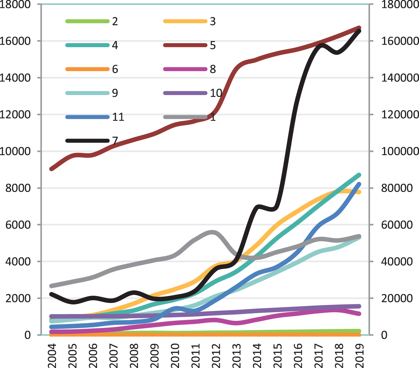
Statistical diagram of industrial structure, transportation infrastructure, population and consumption levels, and investment and trade data.

This paper calculates the gray correlation degree of each index sequence to the freight volume index sequence under the four types of logistics demand influencing factors, and sorts within the group according to the factor classification. Moreover, this article uses the freight volume index sequence as the reference sequence, and other index sequences as the comparison sequence, and uses MatlabR2016a to calculate the gray correlation degree. Due to the different dimensions of each feature data in the statistical data, it is not convenient to establish the correct prediction model. Therefore, in accordance with the steps of gray correlation analysis mentioned, this article first performs dimensionless processing on time series data. In addition, this article adopts the averaging method, which compares the annual statistical value of each series with the mean of the entire series. After the original data is dimensionless, the new data sequence is obtained as shown in Table 3 and Fig. 6:

Table 3

Data after dimensionless processing

	1	2	3	4	5	6
2004	0.65	0.57	0.23	0.22	0.71	0.63
2005	0.70	0.60	0.25	0.25	0.76	0.89
2006	0.80	0.65	0.28	0.28	0.77	0.89
2007	0.86	0.69	0.35	0.33	0.80	0.89
2008	0.91	0.81	0.44	0.38	0.83	0.89
2009	0.97	0.86	0.56	0.47	0.85	0.89
2010	1.16	0.79	0.64	0.54	0.89	0.89
2011	1.25	0.85	0.76	0.64	0.91	0.89
2012	0.99	0.94	0.97	0.82	0.95	1.02
2013	0.94	0.99	1.04	0.97	1.13	1.02
2014	1.01	1.12	1.26	1.21	1.17	1.02
2015	1.08	1.23	1.55	1.49	1.20	1.14
2016	1.17	1.32	1.74	1.73	1.21	1.14
2017	1.15	1.45	1.91	1.98	1.24	1.27
2018	1.20	1.54	2.02	2.22	1.27	1.27
2019	1.17	1.60	2.01	2.46	1.31	1.27
	7	8	9	10	11
2004	0.36	0.24	0.31	0.83	0.16
2005	0.29	0.25	0.35	0.83	0.18
2006	0.33	0.32	0.40	0.84	0.20
2007	0.30	0.41	0.39	0.84	0.25
2008	0.37	0.59	0.44	0.85	0.26
2009	0.32	0.75	0.50	0.87	0.32
2010	0.33	0.91	0.57	0.89	0.53
2011	0.39	1.00	0.68	0.93	0.49
2012	0.58	1.13	0.88	0.98	0.70
2013	0.66	0.90	1.03	1.02	0.96
2014	1.12	1.15	1.23	1.08	1.23
2015	1.14	1.45	1.44	1.12	1.37
2016	2.08	1.62	1.66	1.17	1.67
2017	2.54	1.80	1.89	1.22	2.19
2018	2.50	1.88	2.00	1.26	2.47
2019	2.68	1.60	2.22	1.28	3.03

Fig. 6

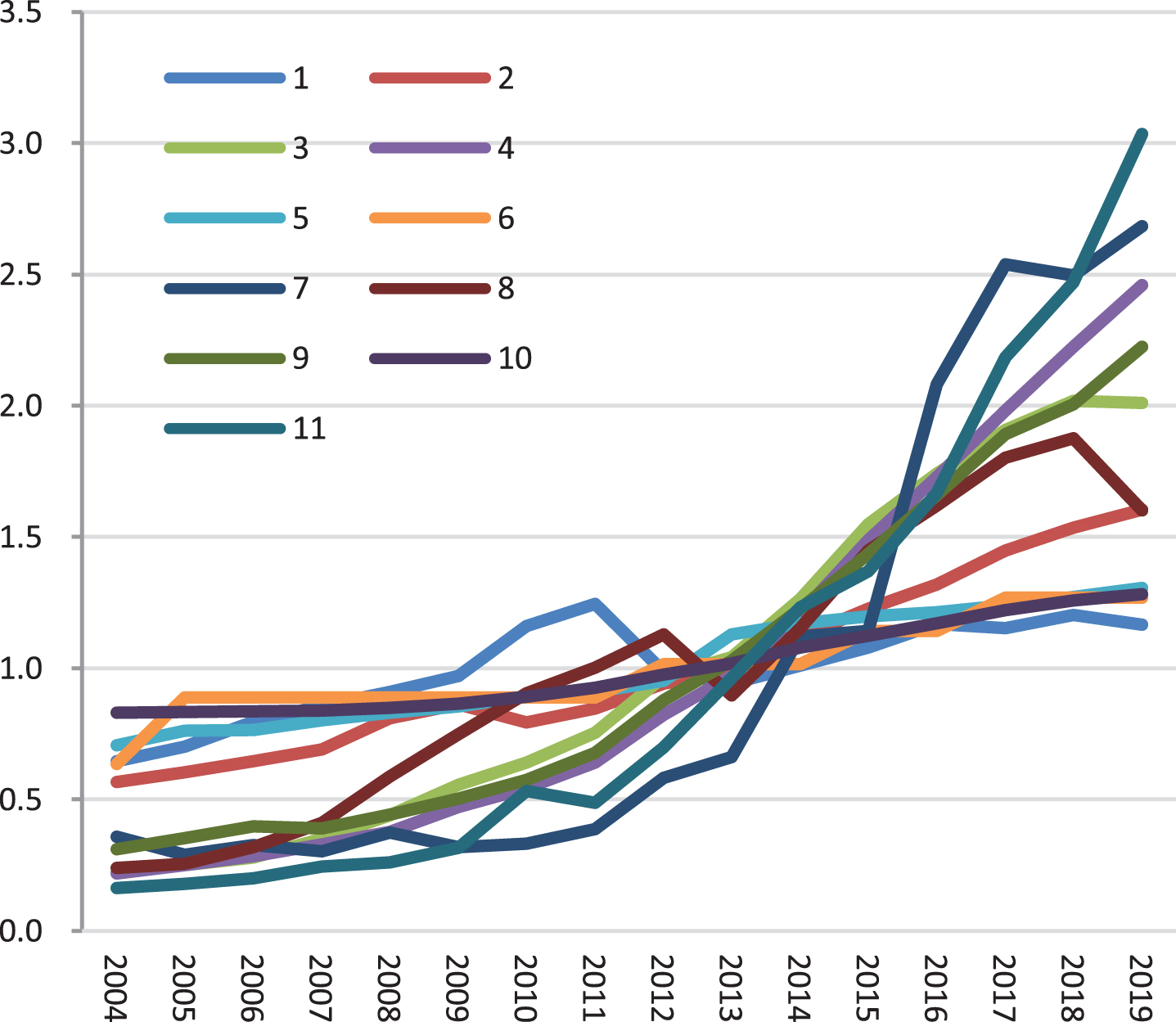
Statistical diagram of data after dimensionless processing.

This paper finds the maximum difference and the minimum difference in each difference sequence from ten difference sequences. After that, this paper compares the maximum difference and minimum difference of ten difference sequences, and obtains the corresponding maximum difference and minimum difference. Then, the result obtained is substituted into the formula to calculate the correlation coefficient, where ρ is 0.5. The results are shown in Table 4 and Fig. 7.

Table 4

Statistical diagram of correlation coefficient

	2	3	4	5	6
2004	0.93	0.70	0.70	0.96	1.00
2005	0.92	0.68	0.68	0.95	0.85
2006	0.87	0.65	0.66	0.98	0.92
2007	0.86	0.66	0.65	0.96	0.98
2008	0.91	0.67	0.65	0.93	0.99
2009	0.91	0.70	0.66	0.90	0.93
2010	0.73	0.65	0.61	0.79	0.79
2011	0.71	0.67	0.62	0.75	0.73
2012	0.97	1.00	0.86	0.98	0.98
2013	0.97	0.92	0.98	0.85	0.94
2014	0.91	0.80	0.84	0.87	1.01
2015	0.88	0.68	0.71	0.90	0.95
2016	0.87	0.63	0.63	0.97	0.99
2017	0.77	0.56	0.54	0.93	0.90
2018	0.75	0.54	0.49	0.95	0.95
2019	0.69	0.53	0.43	0.88	0.91
	7	8	9	10	11
2004	0.78	0.71	0.75	0.85	0.67
2005	0.70	0.69	0.74	0.89	0.65
2006	0.67	0.67	0.71	0.98	0.62
2007	0.64	0.69	0.68	0.99	0.61
2008	0.64	0.75	0.68	0.95	0.60
2009	0.60	0.82	0.68	0.91	0.60
2010	0.54	0.80	0.62	0.79	0.61
2011	0.53	0.81	0.63	0.76	0.56
2012	0.71	0.88	0.91	1.00	0.78
2013	0.78	0.97	0.93	0.94	0.99
2014	0.91	0.88	0.82	0.95	0.82
2015	0.95	0.73	0.73	0.97	0.77
2016	0.51	0.68	0.67	1.01	0.66
2017	0.41	0.60	0.57	0.95	0.48
2018	0.43	0.59	0.55	0.96	0.43
2019	0.39	0.69	0.48	0.90	0.34

Fig. 7

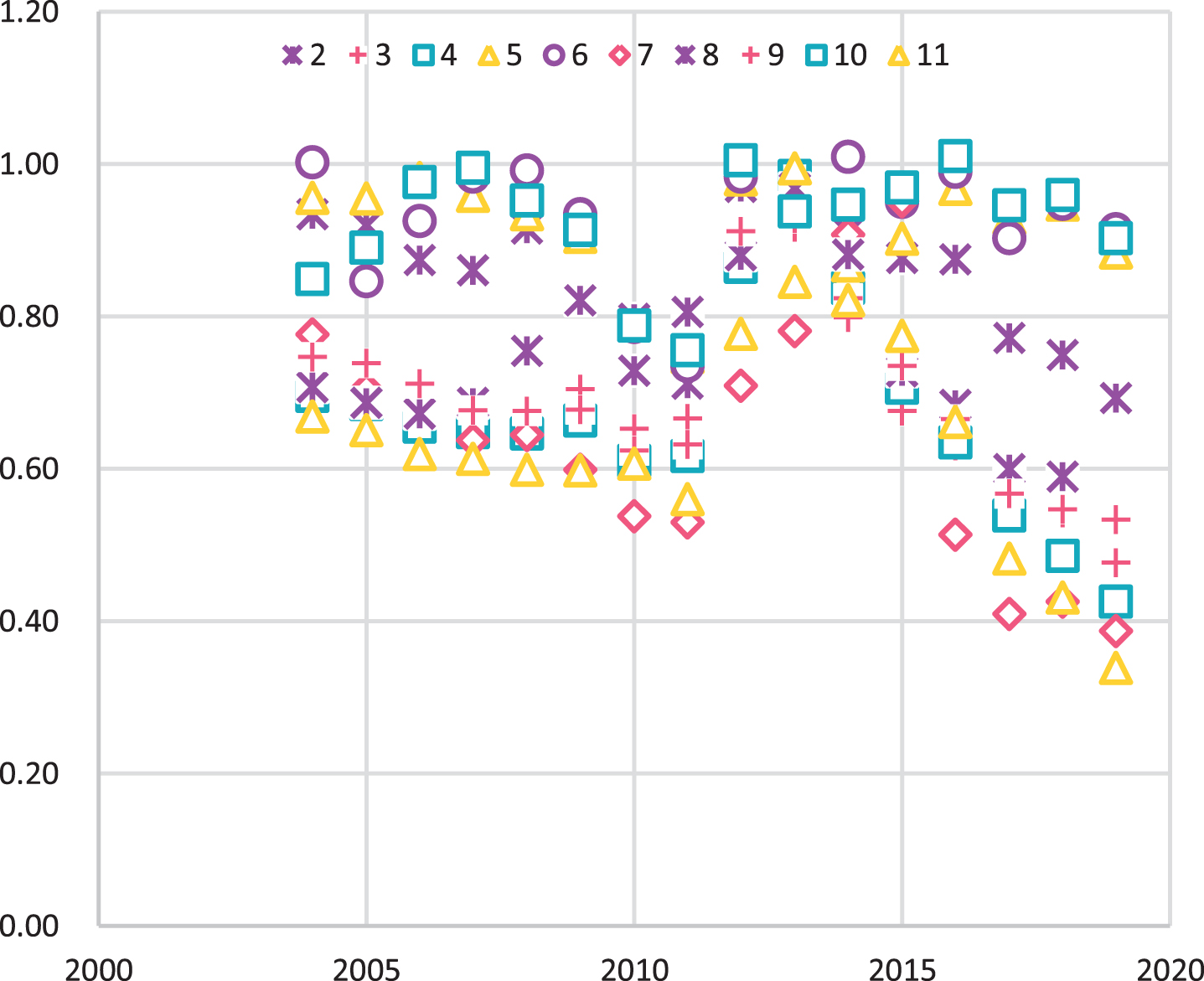
Statistical diagram of correlation coefficient.

The average value of the correlation coefficient of each year is concentrated into one value, which is used as the degree of correlation between the comparison series and the reference series. The calculation results of the correlation degree are shown in Table 5 and Fig. 8:

Table 5

Statistical table of correlation degree

Parameter	Correlation degree
primary industry	0.8453
Secondary industry	0.6889
Tertiary Industry	0.6617
Highway traffic mileage	0.8997
Railway operating mileage	0.9181
Civil aviation route mileage	0.6301
Total foreign trade import and export	0.7395
The total retail sales of social consumer goods	0.6834
permanent residents	0.9153
New investment in fixed assets	0.6306

Fig. 8

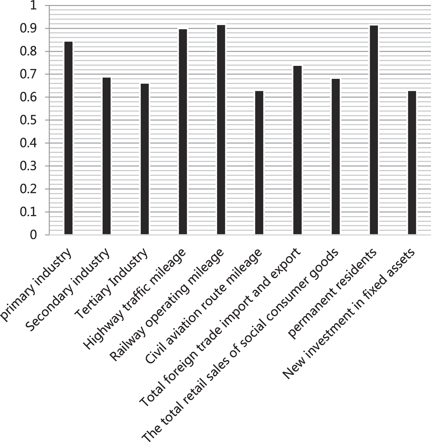
Statistical diagram of correlation degree.

From the above analysis results, we obtain the predicted correlation degree and compare it with actual data. The results show that the model constructed in this paper has good performance and meets the actual needs of the predictive model.

7 Conclusion

From a regional perspective, we can actually see that regional logistics demand is generated in a comprehensive environment. The reason is that logistics activities run through all links of social activities. Therefore, investigating and forecasting the logistics demand of a region is not only a clear grasp of the overall logistics development and supply and demand of the region, but also an understanding of the development of various aspects of the region. This research mainly establishes an index system for logistics demand forecasting. First of all, this research summarizes the 10 main relevant factors that the predecessors found when studying logistics demand by consulting relevant literature. After that, this study uses the grey relational analysis method to give the degree of relevance between each influencing factor and logistics demand, and selects factors with a degree of relevance greater than 0.7 as the indicator of urban logistics demand forecast in this research, including railway operating mileage, permanent population, highway mileage, primary industry output value and total foreign trade import and export. From the prediction results, it can be seen that the model constructed in this paper has good performance and has certain practical effects.

References

Fredriksson

and Liljestrand

, Capturing food logistics: a literature review and research agenda[J], International Journal of Logistics Research and Applications 18(1) (2015), 16–34.

P.J.

and Lin

K.C.

, Unstructured big data analytics for retrieving e-commerce logistics knowledge[J], Telematics and Informatics 35(1) (2018), 237–244.

Pournader

, Shi

, Seuring

, et al., Blockchain applications in supply chains, transport and logistics: a systematic review of the literature[J], International Journal of Production Research 58(7) (2020), 2063–2081.

Lee

C.K.M.

, Lv

, Ng

K.K.H.

, et al., Design and application of Internet of things-based warehouse management system for smart logistics[J], International Journal of Production Research 56(8) (2018), 2753–2768.

Oberhofer

and Dieplinger

, Sustainability in the transport and logistics sector: Lacking environmental measures[J], Business Strategy and the Environment 23(4) (2014), 236–253.

Pamučar

and Ćirović

, The selection of transport and handling resources in logistics centers using Multi-Attributive Border Approximation area Comparison (MABAC)[J], Expert Systems with Applications 42(6) (2015), 3016–3028.

Senthil

, Srirangacharyulu

and Ramesh

, A robust hybrid multi-criteria decision making methodology for contractor evaluation and selection in third-party reverse logistics[J], Expert Systems with Applications 41(1) (2014), 50–58.

Niknejad

and Petrovic

, Optimisation of integrated reverse logistics networks with different product recovery routes[J], European Journal of Operational Research 238(1) (2014), 143–154.

García-Arca

, Prado-Prado

J.C.

and Garrido

, “Packaging logistics”: promoting sustainable efficiency in supply chains[J], International Journal of Physical Distribution & Logistics Management 44(4) (2014), 325–346.

10.

Leuschner

, Carter

C.R.

, Goldsby

T.J.

, et al., Third-party logistics: a meta-analytic review and investigation of its impact on performance[J], Journal of Supply Chain Management 50(1) (2014), 21–43.

11.

Roghanian

and Pazhoheshfar

, An optimization model for reverse logistics network under stochastic environment by using genetic algorithm[J], Journal of Manufacturing Systems 33(3) (2014), 348–356.

12.

Tadić

, Zečević

and Krstić

, A novel hybrid MCDM model based on fuzzy DEMATEL, fuzzy ANP and fuzzy VIKOR for city logistics concept selection[J], Expert Systems with Applications 41(18) (2014), 8112–8128.

13.

Rezaei-Malek

and Tavakkoli-Moghaddam

, Robust humanitarian relief logistics network planning[J], Uncertain Supply Chain Management 2(2) (2014), 73–96.

14.

Petersen

, Hackius

and von See

, Mapping the sea of opportunities: Blockchain in supply chain and logistics[J], it-Information Technology 60(5-6) (2018), 263–271.

15.

Kaur

and Singh

S.P.

, Sustainable procurement and logistics for disaster resilient supply chain[J], Annals of Operations Research 283(1) (2019), 309–354.

16.

Pedrosa

, Blazevic

and Jasmand

, Logistics innovation development: a micro-level perspective[J], International Journal of Physical Distribution & Logistics Management 45(4) (2015), 313–332.

17.

Alkhatib

S.F.

, Darlington

, Yang

, et al., A novel technique for evaluating and selecting logistics service providers based on the logistics resource view[J], Expert Systems with Applications 42(20) (2015), 6976–6989.

18.

Wang

, Ma

, Lao

, et al., A fuzzy-based customer clustering approach with hierarchical structure for logistics network optimization[J], Expert Systems with Applications 41(2) (2014), 521–534.

19.

de Keizer

, Akkerman

, Grunow

, et al., Logistics network design for perishable products with heterogeneous quality decay[J], European Journal of Operational Research 262(2) (2017), 535–549.

20.

Dablanc

, Ogilvie

and Goodchild

, Logistics sprawl: differential warehousing development patterns in Los Angeles, California, and Seattle, Washington[J], Transportation Research Record 2410(1) (2014), 105–112.

21.

Sathish

, Profit maximization in reverse logistics based on disassembly scheduling using hybrid bee colony and bat optimization[J], Transactions of the Canadian Society for Mechanical Engineering 43(4) (2019), 551–559.

22.

Moghaddam

K.S.

, Fuzzy multi-objective model for supplier selection and order allocation in reverse logistics systems under supply and demand uncertainty[J], Expert Systems with Applications 42(15-16) (2015), 6237–6254.

23.

Vanovermeire

, Sörensen

, Van Breedam

, et al., Horizontal logistics collaboration: decreasing costs through flexibility and an adequate cost allocation strategy[J], International Journal of Logistics Research and Applications 17(4) (2014), 339–355.

24.

Morganti

and Gonzalez-Feliu

, City logistics for perishable products. The case of the Parma’s Food Hub[J], Case Studies on Transport Policy 3(2) (2015), 120–128.

25.

Montoya-Torres

J.R.

, Muñoz-Villamizar

and Vega-Mejía

C.A.

, On the impact of collaborative strategies for goods delivery in city logistics[J], Production Planning & Control 27(6) (2016), 443–455.