Control loop oscillation detection and quantification using PRONY method of IIR filter design and deep neural network

Abstract

Generally, the process industry is affected by unwanted fluctuations in control loops arising due to external interference, components with inherent nonlinearities or aggressively tuned controllers. These oscillations lead to production of substandard products and thus affect the overall profitability of a plant. Hence, timely detection of oscillations is desired for ensuring safety and profitability of the plant. In order to achieve this, a control loop oscillation detection and quantification algorithm using Prony method of infinite impulse response (IIR) filter design and deep neural network (DNN) has been presented in this work. Denominator polynomial coefficients of the obtained IIR filter using Prony method were used as the feature vector for DNN. Further, DNN is used to confirm the existence of oscillations in the process control loop data. Furthermore, amplitude and frequency of oscillations are also estimated with the help of cross-correlation values, computed between the original signal and estimated error signal. Experimental results confirm that the presented algorithm is capable of detecting the presence of single or multiple oscillations in the control loop data. The proposed algorithm is also able to estimate the frequency and amplitude of detected oscillations with high accuracy. The Proposed method is also compared with support vector machine (SVM) and empirical mode decomposition (EMD) based approach and it is found that proposed method is faster and more accurate than the later.

Keywords

Oscillation detection Prony method EMD IIR filter deep neural network cross-correlation SVM

1 Introduction

Process control loops in process industry are very much susceptible to the control loop oscillations. These oscillations in control loops can arise due internal or external factors. These oscillations negatively impact the performance of the loop. This impact can lead to inferior product quality, reduction in profit margin of the plant and increase in threat to property and precious human lives [1 –4]. Presence of oscillations could be attributed to a multitude of factors like non-linear characteristics of the system in question, external disturbances which can cause a variation in the process variable (PV), consequences triggered due to mechanical wear and tear of moving parts, faulty controller parameters and inherent non-linearities present in the final control element like control valves. In a large process plant there could be thousands of control loops and to monitor each one of them manually is a challenging task. Hence, a fast and easy to implement automatic oscillation detection algorithms are highly desirable [5]. In the past two decades many algorithms for oscillation detection have been published by several researchers. Therefore, a brief literature survey of the work done in this domain for past decade is presented here.

Heuristic nature of oscillation detection algorithms has been observed and reported by several researchers due to lack of clear mathematical descriptions of oscillations [6]. Li et al. proposed an algorithm based on discrete cosine transform (DCT) and regularity of zero-crossing index for multiple oscillation detection and their parameter estimation [7]. Sivalingam et al. proposed the cross-wavelet transform based method in order to diagnose multiple oscillations [8]. Srinivasan et al. presented a modified empirical mode decomposition (EMD) technique to detect multiple or single oscillations in data [9]. Wang et al. used improved DCT method involving a fitness index for extracting dominant oscillations and hypothesis test on magnitude of oscillations in real time univariate time series data [10].

Naghoosi et al. proposed the peak recognition and clustering method of auto correlation function to detect oscillations in control loop data [11]. Guo et al. presented a method based on improved wavelet packet transform and Shannon entropy to detect multiple or single oscillations in process control loop data [12]. Wardana presented the variational mode decomposition method for plant performance monitoring and oscillation detection [13]. Xun et al. proposed a time varying oscillation detection method using improved local mean decomposition technique [14]. Xie et al. proposed an online tool for fluctuation detection in control loop data with the help of intrinsic time scale decomposition along with a zero crossing algorithm [15]. Yan et al. used a hidden Markov model for detecting repeated patterns in time series data for oscillation detection [16]. Naghoosi et al. proposed a wavelet transform based algorithm for identification and characterization of frequencies of oscillations present in the control loop data [17]. Sharma et al. presented a machine learning based method for the detection of oscillations in control loop data with the help of artificial neural networks. They used linear predictive coefficients based feature vector for determining the presence of oscillations [18].

From the literature survey presented above, two important conclusions can be drawn: 1) Automatic detection and parameter estimation of oscillations in control loop data are necessary for satisfactory operation at any process plant; 2) A good oscillation detection algorithm must have features like high detection accuracy and less computational complexity. Further, it has been observed that negligible work has been reported in literature using artificial intelligence (AI) techniques for detection of oscillations in control loop data. In this presented work, a method for oscillation detection and parameter estimation with the help of Prony’s method of IIR filter design and deep neural network (DNN) has been presented. The proposed method first finds the denominator polynomial coefficients (DPCs) of the IIR filter obtained from Prony’s method and then use them as a feature vector for DNN to confirm the presence of oscillations in the control loop data. Amplitude and frequency of detected oscillations are estimated with the help of cross-correlation between original signal and estimated error signal. The proposed method has been evaluated with the help of real plant and simulated data. Industrial data provided by the Jelali and Huang [6] was used to train the DNN. This work also presents a comparative study between proposed method and EMD based approach [9]. EMD based approach has been used by several researchers for the comparison purpose in recent years. It can be noted that it has become a kind of benchmark method. We also have used EMD based approach for comparative study in our work due to its wide applicability for comparison purpose. Proposed algorithm was compared with EMD based approach for three performance indices: (i) Time taken in oscillation detection (or computational complexity), (ii) Amplitude estimation accuracy and (iii) Frequency estimation accuracy. Proposed algorithm outperforms the EMD based approach in all three indices mentioned above. Comparison results for simulated examples have been shown later in the paper. Major contributions of the presented work have been listed as follows:

Development of a new and simple machine learning approach using DNN for oscillation detection in control loop data.

Noise performance comparison between DNN and support vector machine (SVM) for oscillation detection.

Improvement in speed of oscillation detection.

Improved accuracy in estimation of amplitude and frequency of detected oscillations.

Organisation of rest of the work is as follows: Section 2 describes the mathematics behind Prony analysis and time domain design of IIR filter using Prony method, Section 3 elaborates the proposed oscillation detection method using DNN and also describe the procedure for quantification of frequency and amplitude of detected oscillations, Experimental results have been provided in Section 4 and Section 5 concludes the paper with possible direction of future work.

2 Prony method

In this section the basic underlying mathematics of Prony analysis and IIR filter design using Prony method has been presented.

2.1 Basic Prony analysis

The principle of Prony analysis is based on the procedure of finding a linear combination of exponentials for a given signal [19, 20]. Thus, any signal y (t) can be modelled as a sum of k exponentials. The model can be written mathematically as follows: $y (t) ≅ \hat{y} (t) = \sum_{i = 1}^{k} B_{i} e^{λ_{i} t}$ (1) where, λ_i and B_i are complex numbers and $\hat{y} (t)$ is the estimated signal. Further, k is the system order and B_i is the residue of pole λ_i. The discrete time representation of Equation (1) can be given as: $\hat{y} (nT) = \sum_{i = 1}^{k} B_{i} z_{i}^{n}, n = 0, 1, 2 \dots N - 1$ (2) $z_{i} = e^{λ_{i} T}$ (3) where, z_i : discrete time poles, N : sequence length, n : sample index, and T : sampling interval. The main purpose is to find the values of B_i and z_i, which can result in estimating the signal $y (nT) ≅ \hat{y} (nT)$ for all values of n. On expanding Equation (2) following set of linear equations can be obtained for every value of n: $\begin{matrix} y (0) = B_{1} + B_{2} + \dots B_{k} \\ y (1) = B_{1} z_{1} + B_{2} z_{2} + \dots B_{k} z_{k} \\ ⋮ \\ y (N - 1) = B_{1} z_{1}^{N - 1} + B_{2} z_{2}^{N - 1} + \dots + B_{k} z_{k}^{N - 1} \end{matrix}$ (4)

$\begin{matrix} [\begin{matrix} y (0) \\ \begin{matrix} y (1) \\ ⋮ \\ y (N - 1) \end{matrix} \end{matrix}] \\ = [\begin{matrix} z_{1}^{0} & z_{2}^{0} & \begin{matrix} \dots & z_{k}^{0} \end{matrix} \\ z_{1}^{1} & z_{2}^{1} & \begin{matrix} \dots & z_{k}^{1} \end{matrix} \\ \begin{matrix} ⋮ \\ z_{1}^{N - 1} \end{matrix} & \begin{matrix} ⋮ \\ z_{2}^{N - 1} \end{matrix} & \begin{matrix} \begin{matrix} ⋮ & ⋮ \end{matrix} \\ \begin{matrix} \dots & z_{k}^{N - 1} \end{matrix} \end{matrix} \end{matrix}] [\begin{matrix} B_{1} \\ B_{2} \\ \begin{matrix} ⋮ \\ B_{k} \end{matrix} \end{matrix}] \end{matrix}$ (5)

Equation (5) can be written in compact form in the following way: $Y = ZB$ (6) where, Y is N × 1 vector of signal values, Z is N × k matrix of discrete time poles and B is the k × 1 vector of residues. If one obtains the values of z_i then values of λ_i can be obtained from Equation (3). It can be seen clearly from Equation (6) that to find the values of z_i, N should be greater than 2k (N ⩾ 2k + 1). Further, a k^th order polynomial function (f (z)) with coefficients a_i is assumed with z_i as its roots. f (z) is also known as characteristic polomial. Equation 7 can be constructed with the following assumption. $\begin{matrix} f (z) = (z - z_{1}) (z - z_{2}) \dots (z - z_{k}) \\ = z^{k} - (a_{1} z^{k - 1} + a_{2} z^{k - 2} + \dots + a_{k} z^{0}) = 0 \end{matrix}$ (7)

Now, a 1xN matrix can be constructed as follows: $A = [- a_{k} - a_{k - 1} \dots - a_{1} 10 \dots 0]$ (8)

Multiplying Equation (6) on both sides by A and rearranging, yields: $\begin{matrix} AY = y (k) - [a_{1} y (k - 1) + \dots + a_{k} y (0)] \\ = AZB \end{matrix}$ (9)

$AY = B_{1} [z_{1}^{k} - (a_{1} z_{1}^{k - 1} + a_{2} z_{2}^{k - 2} + \dots + a_{k} z_{1}^{0})] + \dots .$ (10)

$AY = 0$ (11)

Equation (11) can be derived based on the fact that Equation (7) is satisfied by each value of z_i. Equation (11) can also be applied repeatedly to form Equation (12) as follows:

$\begin{matrix} [\begin{matrix} y (k - 1) & y (k - 2) & \dots & y (0) \\ y (k - 0) & y (k - 1) & \dots & y (1) \\ ⋮ & ⋮ & ⋮ & ⋮ \\ y (N - 2) & y (N - 3) & \dots & y (N - k - 1) \end{matrix}] [\begin{matrix} a_{1} \\ a_{2} \\ ⋮ \\ a_{k} \end{matrix}] \\ = [\begin{matrix} y (k + 0) \\ y (k + 1) \\ ⋮ \\ y (N - 1) \end{matrix}] \end{matrix}$ (12)

On careful observation, Equation (12) can be seen as a linear prediction model and the aforementioned equation will have a single solution for the condition N ⩾ 2k + 1, and values of a_i can be determined using least squares problem. Once the values of a_i are calculated, using Equation (7) the values of z_i can be calculated and then values ofλ_i can be calculated using Equation (3). Lastly, values of B_i can be computed using Equation (5).

2.2 Prony method for design of IIR filter

The method for IIR filter design with prescribed time-domain response with the help of Prony analysis is addressed here [21]. Prony method gives an extra dimension for IIR filter design based on time-domain specifications. Equation (13) shows the transfer function of an IIR filter. $\begin{matrix} H (z) = \frac{B (z)}{A (z)} \\ H (z) = \frac{b_{0} + b_{1} z^{- 1} + b_{2} z^{- 2} + \dots + b_{M} z^{- M}}{1 + a_{1} z^{- 1} + \dots + a_{L} z^{- L}} \end{matrix}$ (13) where, M is the numerator polynomial order and L is the denominator polynomial order of Equation (13). H (z) can be related to the impulse response h (n) by the z-transform as shown in Equation (14). $H (z) = \sum_{n = 0}^{\infty} h (n) z^{- n}$ (14)

Further, Equation (13) can be modified as follows: $B (z) = H (z) A (z)$ (15)

Equation (15) is obtained by taking z-transform of the convolution between a(n) andh (n). The convolution can be further written in matrix multiplication form using first q+1 terms of the impulse response. $[\begin{matrix} b_{0} \\ b_{1} \\ \begin{matrix} b_{2} \\ ⋮ \\ \begin{matrix} b_{M} \\ 0 \\ \begin{matrix} ⋮ \\ 0 \end{matrix} \end{matrix} \end{matrix} \end{matrix}] = [\begin{matrix} \begin{matrix} h_{0} & 0 & 0 \\ h_{1} & h_{0} & 0 \\ h_{2} & h_{1} & h_{0} \end{matrix} & \dots & \begin{matrix} 0 \\ 0 \\ 0 \end{matrix} \\ \begin{matrix} ⋮ & ⋮ & ⋮ \end{matrix} & ⋱ & ⋮ \\ \begin{matrix} h_{M} & ⋮ & ⋮ \\ ⋮ & ⋮ & ⋮ \\ h_{q} & \dots & \dots \end{matrix} & \dots & \begin{matrix} ⋮ \\ ⋮ \\ h_{q - L} \end{matrix} \end{matrix}] [\begin{matrix} 1 \\ a_{1} \\ \begin{matrix} a_{2} \\ ⋮ \\ a_{L} \end{matrix} \end{matrix}]$ (16)

In order to find the values of b_i and a_i, the matrices can be partitioned to give: $[\begin{matrix} b \\ \dots \\ 0 \end{matrix}] = [\begin{matrix} H_{1} \\ \dots \dots \dots \dots \\ \begin{matrix} h_{1} & ⋮ & H_{2} \end{matrix} \end{matrix}] [\begin{matrix} 1 \\ \dots \\ a \end{matrix}]$ (17)

In Equation (17) the matrix b represents the M + 1 numerator coefficients of Equation (13) and a represents the denominator coefficients of Equation (13), h ₁ is the vector of the last (q - M) terms of the impulse response, H₁ is the (M + 1) by (L + 1) partition of Equation (16) and H₂ is the remaining (q - M) by L part of the matrix of Equation (16). The lower half of the Equation (16) representing the (q - M) equations is written as: $0 = h_{1} + H_{2} a \Rightarrow h_{1} = - H_{2} a$ (18)

The upper (M + 1) equations of Equation (17) are written as follows: $b = H_{1} a$ (19)

Equation (19) directly computes the coefficient matrix b . Under the condition, q = L + M, H₂ is a square matrix then Equation (18) can only be solved for a if, H₂ is non-singular. Once a is calculated then using Equation (19) the numerator coefficients b can be calculated. If H₂ is considered as singular, then Equation (18) may have many possible solutions and lower order system can be used to generate h (n).

In this work, above describe method to design IIR filter using Prony method has been used to develop a control loop oscillation detection and parameter quantification algorithm. This method estimates the H (z) with desired number of poles and zeros assuming time domain data under consideration as the impulse response h (n) of the filter. Further, detailed description of the proposed algorithm is given in forthcoming section.

3 Proposed algorithm

Description of the steps involved in proposed oscillation detection and parameter quantification algorithm using IIR filter design by Prony method has been presented in this section.

3.1 Step 1: Pre-processing

It has been observed that set point (SP) variation and external disturbances often corrupt the control loop data. The former one introduces the slow varying trend in the measured PV Data of control loop. Accurate detection of oscillations requires removal of these slow varying trends. This can be achieved by pre-processing the data prior to using it for oscillation detection purpose. There are several methods available for removing these slow varying trends from the data. In this work best fit line to the measure data was subtracted from itself in order to remove the slow varying non-stationary trend.

3.2 Step 2: Extraction of denominator polynomial of an IIR filter

Description of the steps involved in oscillation detection in control loop data is given in the following sub-sections.

3.2.1 IIR filter design

With the aid of Prony method, an IIR filter is designed whose transfer function H (z) is given by Equation (13). The impulse response of the designed filter h (n) approximates the input data. As mentioned by Jelali and Huang [6], process control loop oscillation detection algorithms are heuristic in nature due to lack of available mathematical description. Order of numerator and denominator are considered to be a reasonably optimal choice after observing their effect in several experimental trials. Numerator and denominator were considered as 5^th order polynomial while describing the relation between DPC (a) and presence of oscillations in the control loop data in next paragraph.

3.2.2 Relation between denominator polynomial coefficients and presence of oscillation

After finding the denominator coefficients a, denominator polynomial A (z) is reconstructed and its roots r, which are essentially the poles of H (z), are obtained. These roots can be represented on z-plane as roots of A (z) are complex in nature. It was noticed that the roots of A (z) were lying very close to the unit circle if the signal under observation is oscillatory in nature. Thus, the presence of oscillations in control loop data can be investigated with the help of information about roots’ location on z-plane. In the case of oscillatory impulse response (problem under consideration) the obtained IIR filter will be marginally stable. Hence, one or more poles of the IIR filter or roots of the denominator polynomial will lie on the unit circle. This is also evident from the Fig. 1, in which some of IIR filter poles lies on the unit circle for a pure sinusoidal oscillatory signal. Further, it was observed that for a noisy oscillatory signal, poles of the IIR filter don’t lie on the unit circle anymore but lies in the region very close to the unit circle.

Fig. 1

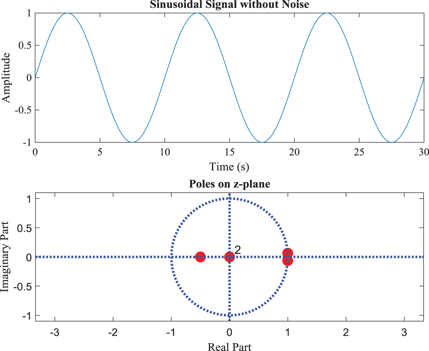
Sinusoidal signal and poles of obtained IIR filter on z-plane.

Same is evident from the Fig. 2 too, in which poles of IIR filter has been shown on z-plane for a noisy oscillatory sinusoidal signal. Distance of the poles from the unit circle further depends upon the presence of noise in the signal under observation. Hence, it can be said that vector a inherits oscillatory information of the signal and can be used for the oscillation detection purpose. Keeping this in mind it can be concluded that machine learning algorithm can be utilized here for the purpose of decision making about the presence or absence of the oscillations in the control loop data.

Fig. 2

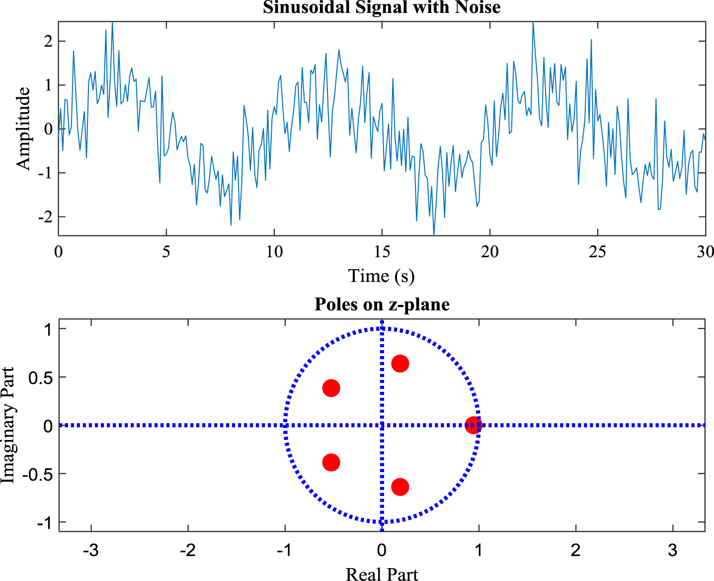
Noisy sinusoidal signal and poles of obtained IIR filter on z-plane.

3.3 Step 3: Oscillation detection using DNN

As explained in the previous step, DPCs of the obtained IIR filter contain the information about presence of oscillation in the control loop data. Artificial intelligence techniques like DNN can be utilized to decide the presence or absence of oscillations in the control loop data based on the DPCs. DNN is the extension of artificial neural network with more than one hidden layers. DNN based method of oscillation detection involves two phases: (i) training phase and (ii) testing phase. This procedure has been shown with the help of a block diagram in Fig. 3. In training phase DPC features are extracted from the training data set and DNN is trained with the help of supervised learning. During the training phase, training data set was divided into three different data sets: (i) training, (ii) testing and (iii) validation. This is done in order to train DNN more effectively.

Fig. 3

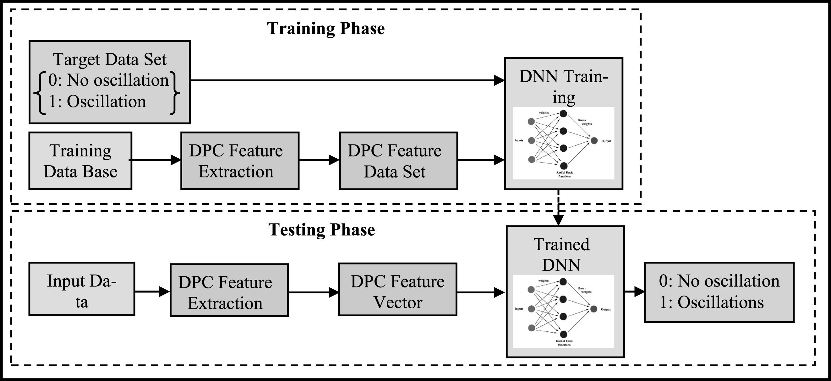
Graphical representation of oscillation detection method based on DNN.

In testing phase trained DNN is used to identify the presence or absence of oscillations in input data and this is done by extracting the DPC feature vector from input data and then feeding it to the trained DNN. It should be noted that in testing phase new data (which was not the part of training data set) is used to test the performance of trained DNN. Further, DNN gives output in the form of 0 or 1 corresponding to absence or presence of oscillations in the input data. In this step 3, data set description, feature vector extraction, and training of DNN has been described.

3.3.1 Training data base

In machine learning approach, performance of the classifier depends upon its training which ultimately depends upon the training data base. Larger the training data base better will be the performance of the classifier. In this work raw industrial data provided by Jelali and Huang [6] was used to create training data base. Raw industrial data contains control loop data from several processes like flow, pressure, level, concentration etc., having oscillations due to stiction, external disturbances and controller tuning. Some control loop data was having no oscillations as well.

Training data base was created from this raw industrial data with the following procedure: (i) SP was subtracted from process variable (PV) in order to get error data without SP bias. (ii) Normalization was done of the obtained error data so that amplitude variation remains within the range of –1 to+1. (iii) Finally normalized error data was split into several little parts in a way that each part accommodates at least two or three oscillation cycles. This division of data was done to create much larger data set for training of DNN. Further, it should be noted that, non-uniform division was done as sampling frequency, data length and oscillation frequency were different for different control loop data.

Information about control loop name, type of oscillation, number of sub-segments done for each control loop and total training data sets formed are given in Table 1. In total 286 data sets were created involving non-oscillatory and oscillatory control loop data. Within these 286 data sets 86 oscillatory data sets were because of disturbances, 132 oscillatory data sets were because of stiction problem in control valves, 17 oscillatory data sets were because of controller tuning and 51 data sets were there without any kind of oscillation. Additionally, target data set was created having dimension of 1x286, in which 1 and 0 was used to indicate oscillatory and non-oscillatory data set respectively. So, in target data set, there were in total 51 zeros corresponding to non-oscillatory data sets and 235 ones corresponding to oscillatory data sets.

Table 1
Control loop name and no. of sub segments for each loop data

S. No. Oscillation Type Control Loop Name No. of Sub-segments Total Training Data Sets Formed

1 Stiction BAS 6 5 132

2 BAS 7 4

3 CHEM 1 4

4 CHEM 5 4

5 CHEM 6 5

6 CHEM 8 2

7 CHEM 10 4

8 CHEM 11 4

9 CHEM 12 2

10 PAP 1 2

11 PAP 2 8

12 PAP 3 6

13 PAP 5 18

14 PAP 12 15

15 PAP 13 9

16 POW 2 17

17 POW 4 17

18 MIN 1 6

19 External Disturbances CHEM 21 15 86

20 CHEM 27 3

21 CHEM 33 15

22 CHEM 36 3

23 CHEM 37 4

24 CHEM 38 2

25 CHEM 39 6

26 PAP 7 12

27 MET 1 4

28 MET 2 22

29 Controller Tuning CHEM 4 5 17

30 PAP 4 12

31 No Oscillation BAS 1 20 51

32 BAS 2 20

33 MET 3 11

S. No.	Oscillation Type	Control Loop Name	No. of Sub-segments	Total Training Data Sets Formed
1	Stiction	BAS 6	5	132
2		BAS 7	4
3		CHEM 1	4
4		CHEM 5	4
5		CHEM 6	5
6		CHEM 8	2
7		CHEM 10	4
8		CHEM 11	4
9		CHEM 12	2
10		PAP 1	2
11		PAP 2	8
12		PAP 3	6
13		PAP 5	18
14		PAP 12	15
15		PAP 13	9
16		POW 2	17
17		POW 4	17
18		MIN 1	6
19	External Disturbances	CHEM 21	15	86
20		CHEM 27	3
21		CHEM 33	15
22		CHEM 36	3
23		CHEM 37	4
24		CHEM 38	2
25		CHEM 39	6
26		PAP 7	12
27		MET 1	4
28		MET 2	22
29	Controller Tuning	CHEM 4	5	17
30		PAP 4	12
31	No Oscillation	BAS 1	20	51
32		BAS 2	20
33		MET 3	11

3.3.2 Feature extraction

Input data contains lot of samples and hence cannot be used to train the DNN directly, instead features are extracted from the data and these extracted features are used for training and testing of DNN. Further, features are hidden information within the data based on which any specific decision can be taken. In the underline problem of oscillation detection, poles of the obtained IIR filter have the information about the presence of oscillations and hence denominator coefficients (a) of the designed IIR filter were used as a feature vector to train the DNN. As described in previous step, ten denominator coefficients will be extracted from each training data set given in Table 1 and will form the feature vector for input data.

3.3.3 DNN architecture

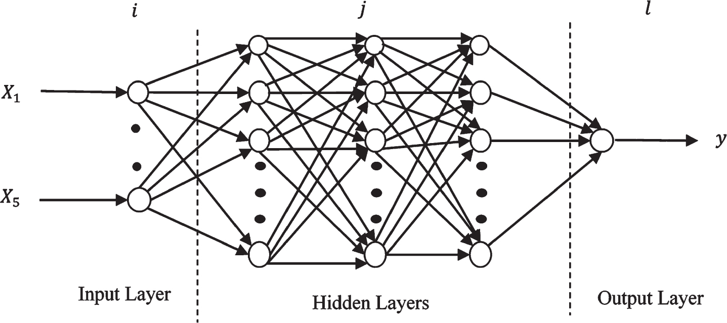
As described before, DNN is the extension of ANN with more than one hidden layers. Figure 4 shows the DNN architecture used in presented work. DNN contains three layers named as: input layer, hidden layer and output layer. Input layer of DNN has 10 neurons, equal to the number of features in feature vector, hidden layer consists of three layer of neurons with 15 neurons in each layer and output layer contains only one neuron in order to give 1 or 0 depending upon the presence and absence of oscillations in the input data.

Fig. 4

DNN architecture for proposed work.

3.3.4 DNN training

DNN was trained with the help of feature vectors obtained from the data set described in Table 1. MATLAB^® environment was used to create and train the proposed DNN structure using trainlm algorithm. During training process of the DNN, 90% of the data set was used for training, 5% of the data set was used for validation and 5% of the data set was used for testing purpose. Mean squared error (MSE) performance of the DNN was achieved of 7.147x10^-5. Further, 100% detection accuracy was obtained in training, validation and testing phase. Confusion matrix for the trained DNN is shown in Fig. 5 and corresponding performance curve are depicted in Fig. 6. This trained DNN has been used further, to detect the oscillations in control loop data.

Fig. 5

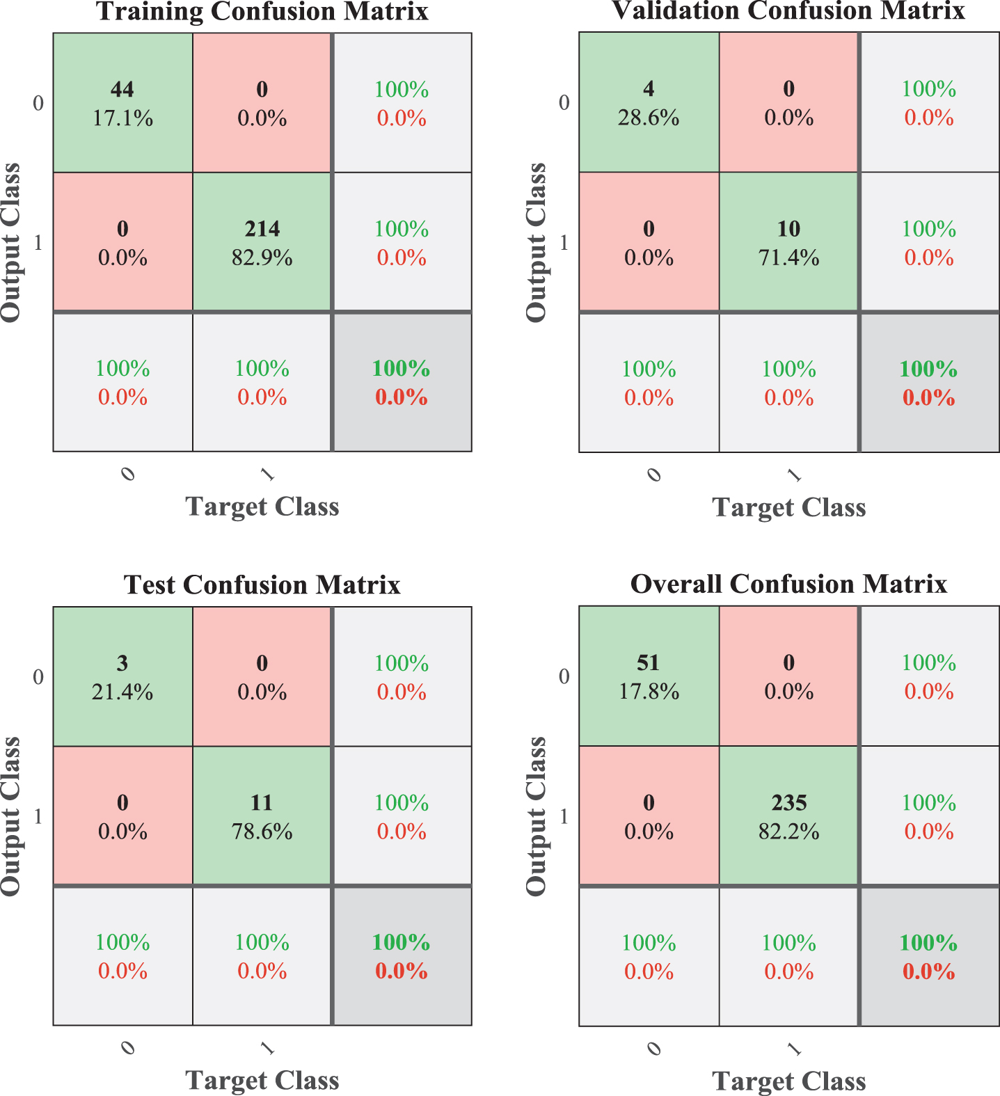
Confusion matrix for the trained DNN.

Fig. 6

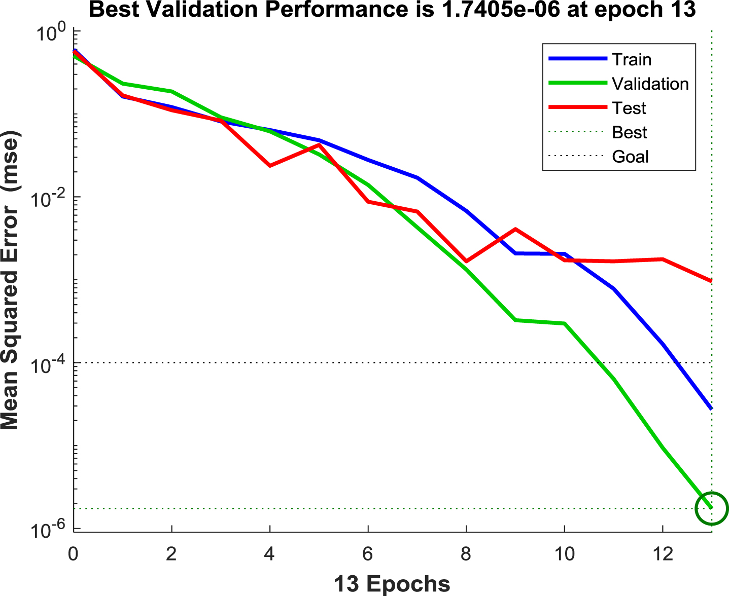
Performance graph of the trained DNN during training stage.

3.4 Step 4: Amplitude and frequency estimation

Steps involved in estimating the frequency and amplitude of detected oscillations are presented here.

3.4.1 Computation of estimated error and cross-correlation

In Prony method of IIR filter design, impulse response of the filter h (n) was supposed to be the original data sequence from which filter transfer function H (z) was obtained. First signal is estimated from the impulse response of the designed filter. Then estimated error ee (n) was calculated between the original signal and estimated signal. Mathematically it can be expressed as follows: $ee (n) = x (n) - \hat{x} (n)$ (20) where, x (n): original signal, $\hat{x} (n)$ : estimated signal and ee (n): estimated error signal. As a next step cross-correlation between estimated error and original signal was computed as per Equation (21). $C_{xee} [l] = \sum_{n = 0}^{P - 1} x [n] ee [n - l]$ (21) $for l = 0, \pm 1, \pm 2 \dots \dots \pm length (ee [n] - 1)$ where, P : input sequence length, l : lag, and C_xee [l] : the cross-correlation value at lag l [23]. Further, cross-correlation values at positive lag points (C_xee [l₊]), were used to estimate the frequency of the oscillation.

3.4.2 Oscillations frequency estimation

As mentioned in previous step, cross-correlation values corresponding to the positive lags (C_xee [l₊]) were selected in order to estimate the oscillation frequency. Now, mean of the selected cross-correlation values was subtracted from them, as per Equation (22). $\bar{C_{xee}} [l_{+}] = C_{xee} [l_{+}] - mean (C_{xee} [l_{+}])$ (22)

This operation removes any false information in the form of a DC bias. After this, magnitude spectrum of resultant cross-correlation was computed with the help of fast fourier transform (FFT). The resultant magnitude spectrum was then normalized as per Equation (23). $\hat{F} [\bar{C_{xee}} [l_{+}]] = \frac{| F [\bar{C_{xee}} [l_{+}]] |}{\max (| F [\bar{C_{xee}} [l_{+}]] |)}$ (23) where, $| F [\bar{C_{xee}} [l_{+}]] | :$ magnitude spectrum of $\bar{C_{xee}} [l_{+}]$ and $\hat{F} [\bar{C_{xee}} [l_{+}]] :$ normalized magnitude spectrum. Peak frequency components in normalized magnitude spectrum having magnitude greater than threshold of 0.2 were considered as the oscillatory frequency components present in the control loop data. It should be noted that this threshold value can be tuned and can be adjusted if prior knowledge of noise power present in the signal is known.

3.4.3 Oscillations amplitude estimation

Oscillation amplitude estimation is the last step in proposed algorithm. For estimating the amplitude of detected oscillations, magnitude spectrum of the original data sequence was computed and magnitude values corresponding to the estimated frequencies (estimated in previous step) were considered as the amplitude of oscillations present in the signal.

Logical flow chart of the proposed oscillation detection and quantification algorithm is shown in Fig. 7.

Fig. 7

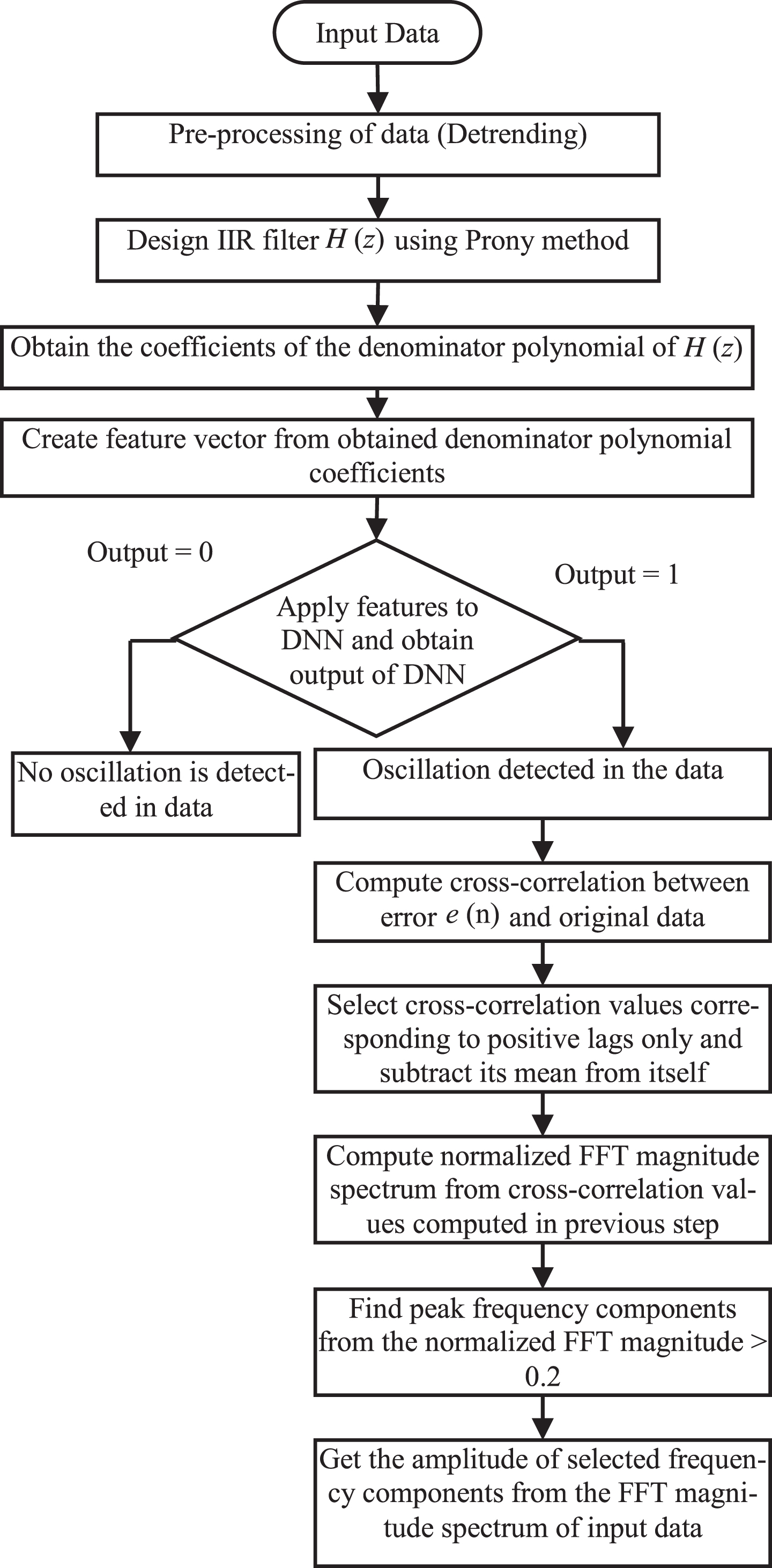
Flow chart of the proposed oscillation detection and quantification algorithm.

4 Results & discussion

Several case studies involving simulated and real plant data have been considered to evaluate the proposed oscillation detection algorithm. Results of all the test cases have been provided in this section.

4.1 Simulation case studies

In simulation case study, four examples with and without oscillations have been considered. Examples 3 and 4 were taken from EMD based approach in order to perform comparative study between proposed method and EMD based method [9]. In simulation cases, additive white gaussian noise (AWGN) was also added to the simulated signal in order to make simulations more realistic. In this simulated study, comparison between DNN and other AI technique named as SVM for oscillation detection was also done. Further, 100 independent runs were performed for every example and results were recorded. Mean value of these runs was considered as the final result and is presented here. It should be noted that, these simulation examples were not used for the training purpose of the DNN and SVM.

4.1.1 Example 1: Data without oscillation

In this example, proposed algorithm was applied on time series data with no oscillations and contains only AWGN with 1.3 variance and zero mean. Figure 8 shows the simulated data without oscillations. Further, obtained feature vector for this example is shown in Table 2. DNN gives 0 for this example on feeding the corresponding feature vector to it.

Fig. 8

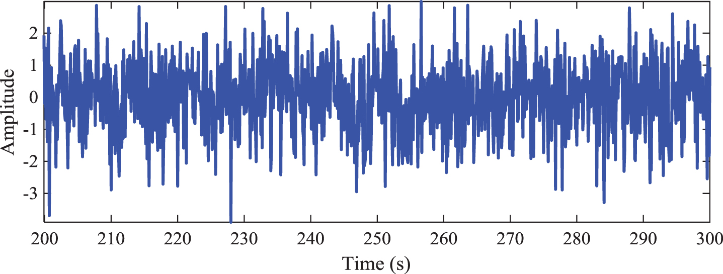
Data without any oscillations: Example 1.

Table 2

Feature vector and output of DNN for simulation studies

Simulation examples	DPC Feature vector for DNN										DNN Output	SVM Output
Example 1	–0.005	0.020	–0.057	–0.026	–0.001	–0.021	–0.007	–0.026	0.005	–0.043	0	0
Example 2 (SNR=10dB)	–0.403	–0.248	–0.190	–0.083	–0.161	0.009	–0.059	0.055	–0.004	0.133	1	1
Example 2 (SNR=7dB)	–0.347	–0.212	–0.164	–0.070	–0.152	0.002	–0.071	0.030	–0.038	0.079	1	1
Example 2 (SNR=5dB)	–0.311	–0.189	–0.147	–0.061	–0.146	–0.003	–0.078	0.015	–0.059	0.045	1	0
Example 2 (SNR=2dB)	–0.251	–0.151	–0.120	–0.046	–0.135	–0.008	–0.088	–0.008	–0.092	–0.008	0	0
Example 3	–0.859	0.096	0.084	0.139	–0.028	0.109	–0.113	–0.021	–0.173	0.054	1	1
Example 4	–0.671	–0.246	0.045	0.132	0.051	0.106	–0.174	–0.142	–0.134	0.147	1	1
Real plant data	–1.015	–0.342	0.081	0.144	0.181	0.044	–0.132	0.021	–0.030	0.070	1	1

4.1.2 Example 2: Sinusoidal signal with noise having different SNRs

In this example, a sinusoidal signal with different amount of noise content was considered to evaluate the oscillation detection ability of proposed algorithm in noisy environment. Signal corrupted with AWGN is given by Equation (24). $y (nT) = sin (2 π fnT) + w (nT)$ (24) where, f : frequency, n : ample number, T : sampling period and w (nT) : AWGN. Frequency of the signal is chosen to be 0.1Hz and sampling interval was set at 0.1s. Figure 9(a)-(d) shows the sinusoidal signal for different signal to noise ratio (SNR) values of 10dB, 7dB, 5dB and 2dB respectively. Table 2 shows the feature vector for different SNR values. It has been noticed that the trained DNN was successfully able to detect oscillations in the data correctly upto SNR of 5dB only. Further, as per the proposed algorithm, frequency of oscillation was estimated to be 0.1Hz with 100% accuracy. Estimated amplitude of oscillation was 0.957, 0.961 and 0.995 for SNR values of 10dB, 7dB and 5dB, respectively. Oscillation amplitude was estimated with 95.7%, 96.1% and 99.5% accuracy for SNR values of 10dB, 7dB and 5dB, respectively. From this example, it is clear that the both DNN and SVM AI techniques are sensitive to the amount of noise present in the input signal.

Fig. 9

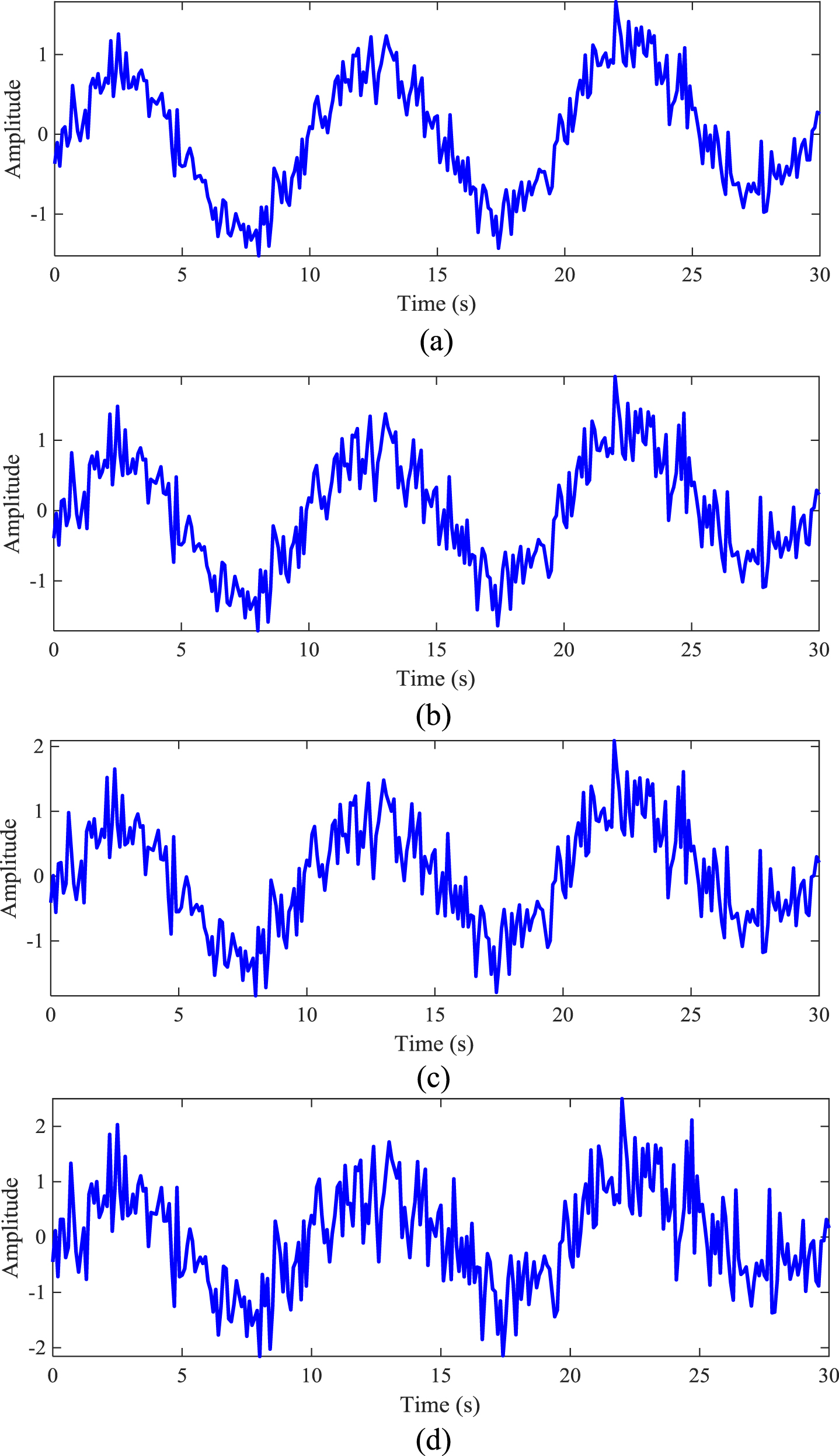
Sinusoidal signal corrupted with AWGN (a) SNR=10dB (b) SNR=7dB (c) SNR=5dB (d) SNR=2dB: Example 2.

Further, it also evident from Table 2 that DNN shows superior noise performance as compared to SVM for oscillation detection in noisy data.

4.1.3 Example 3: Sinusoidal signal corrupted with colored noise

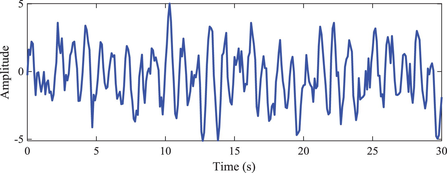
In this example, a sinusoidal signal corrupted using colored noise was studied in order to evaluate the proposed algorithm. Colored noise was obtained after passing AWGN with zero mean and unit variance through a filter with the following transfer function: 1/(1 - 0.7z^-1) . The resultant signal can thus be expressed by Equation (25). $y (nT) = 2 sin (2 π fnT) + c (nT)$ (25) where, T : sampling interval, n : sample index, and c (nT) is the colored noise. Sampling interval for this case was chosen to be 0.1s. Amplitude and frequency of the signal was 2 units and 1Hz, respectively. Figure 10 shows the signal described by Equation (25). Numerical values of the feature vector given in Table 2. Output of the DNN for this feature set was 1 and hence oscillations were detected using the trained DNN. Further, frequency and amplitude of the input data were approximated as 1Hz and 2.0084 units with 100% and 99.58%, accuracy respectively.

Fig. 10

Signal with sinusoidal oscillation and corrupted with colored noise: Example 3.

4.1.4 Example 4: Signal with slow varying trend and multiple oscillations

Signal with slow varying trend and multiple oscillations was considered for this example. Mathematically it is represented by Equation (26).

$\begin{matrix} y (nT) = 0.005 n^{2} + 3 sin (2 π 0.2 nT) \\ + 2 sin (2 π nT) + w (nT), \end{matrix}$ (26) where, n: sample index, T: sampling interval, w (nT) : AWGN with zero mean and 1.3 variance. Sampling interval in this example was chosen to be 0.1s. This signal contains two frequency components of 1Hz and 0.2Hz with amplitudes of 2 units and 3 units, respectively. Figure 11 shows the signal under consideration. Denominator coefficients of the obtained IIR filter as feature vector are tabulated in Table 2. For this example, too, output of the DNN was 1 and hence confirming the oscillations in the signal. Further, frequency and amplitude of the oscillations were computed as per the presented algorithm. Further, frequency of the oscillations was estimated to be 0.2Hz and 1Hz with 100% accuracy and amplitude of the oscillations was estimated to be 3.0161 and 1.9417 with 99.46% and 97.08% accuracy, respectively.

Fig. 11

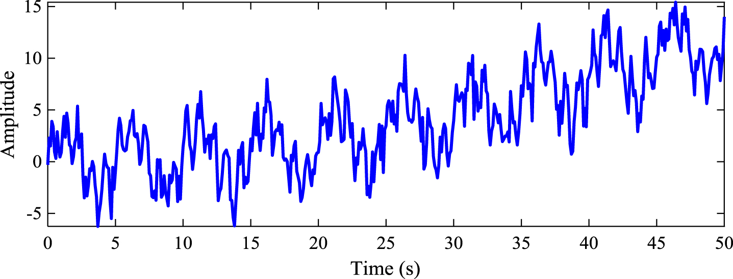
Signal with multiple oscillations and slow varying trend: Example 4.

Example 3 and 4 were further compared to the EMD based approach with speed and accuracy of frequency and amplitude estimation as the comparison metric. For this comparison purpose 100 trials were conducted and result of each trial was stored. Further, mean value of the stored data was considered as the final value. Results of this comparative study have been tabulated in Table 3. Personal computer with Intel^® Core ™ i5 CPU and 8GB RAM was used for this comparative study. Further, results of this comparative study are shown graphically in Fig. 12. Figure 12(a) shows the comparison result of time taken by proposed method and EMD based method, Fig. 12(b) shows the accuracy obtained in both methods for amplitude estimation and Fig. 12(c) shows the accuracy in frequency estimation by both methods.

Table 3

Comparative study summary of Examples 3 & 4 with EMD based approach

Simulation case	Oscillations	Methods	Frequency (F) of oscillation			Amplitude (amp) of oscillation		Timing analysis
			F	STD	Accuracy	Amp	Accuracy	Time taken	STD
			(Hz)		(%)		(%)	(s)
Example 3	Detected	Proposed	1.0	0	100	2.0084	99.58	0.0018	0.0018
		EMD	1.0	0	100	1.6500	82.5	0.0813	0.0252
Example 4 (Multiple Oscillations)	Detected	Proposed	0.2	3.905 x10^–15	100	3.0161	99.46	0.0019	0.0019
			1.0	0	100	1.9417	97.08
		EMD	0.1910	0.7313	95.50	4.7200	42.670	0.0716	0.0237
			1.0235	0.0973	97.65	2.9087	54.565

Fig. 12

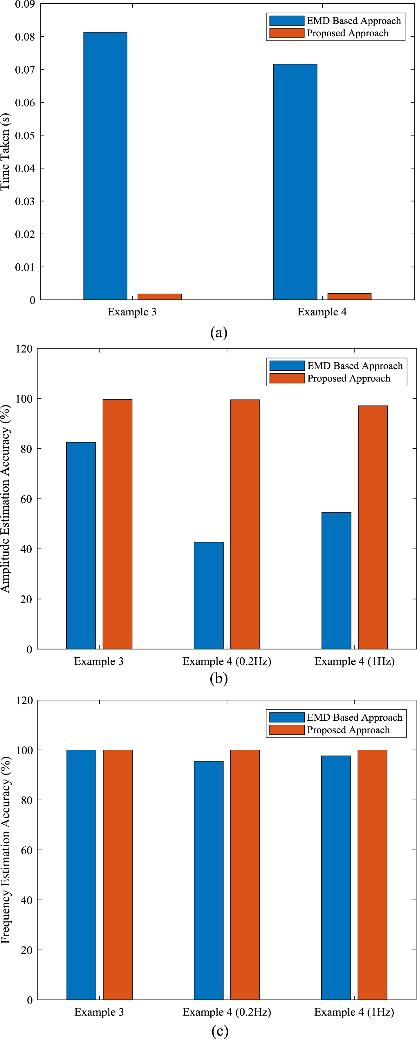
(a) Computational time comparison result (b) Comparison result of estimated amplitude accuracy (c) Comparison result of estimated frequency accuracy.

4.2 Study on real plant data

The proposed method of oscillation detection was also applied to the real plant data. This was done to verify the algorithm in real life scenarios. Oscillatory PV data was recorded from a laboratory scaled flow process plant with a final control element (pneumatic control valve) suffering from stiction nonlinearity [22]. Detailed specifications and description of the plant can be found in [22]. Proportional-Integral (PI) controller with transfer function $G_{c} (s) = \frac{- 3 s - 2.3}{s}$ was used in the plant. PI controlled gain parameters have negative values, as the pneumatic control valve used in the plant is of air-to-close type [22]. PV data was recorded from the plant with sampling interval of 0.1s. Further, it should be noted that, this data was also not used for the training of the DNN.

PV data recorded from the plant was subtracted from the SP in order to remove the SP bias and resultant error signal was considered for further study. Figure 13 shows the error signal from the control loop. Feature vector obtained for this real plant data is shown in Table 2. This feature vector was fed to the trained DNN. Output of the DNN confirmed the presence of oscillations in the input data. Amplitude and frequency of oscillation were estimated as 1.6389 units and 0.1222Hz respectively. Further, comparative study with EMD based approach is given in Table 4. The EMD based approach was unable to detect oscillations in real flow process plant data. This comparison clearly shows that the proposed algorithm is superior to the EMD based approach.

Fig. 13

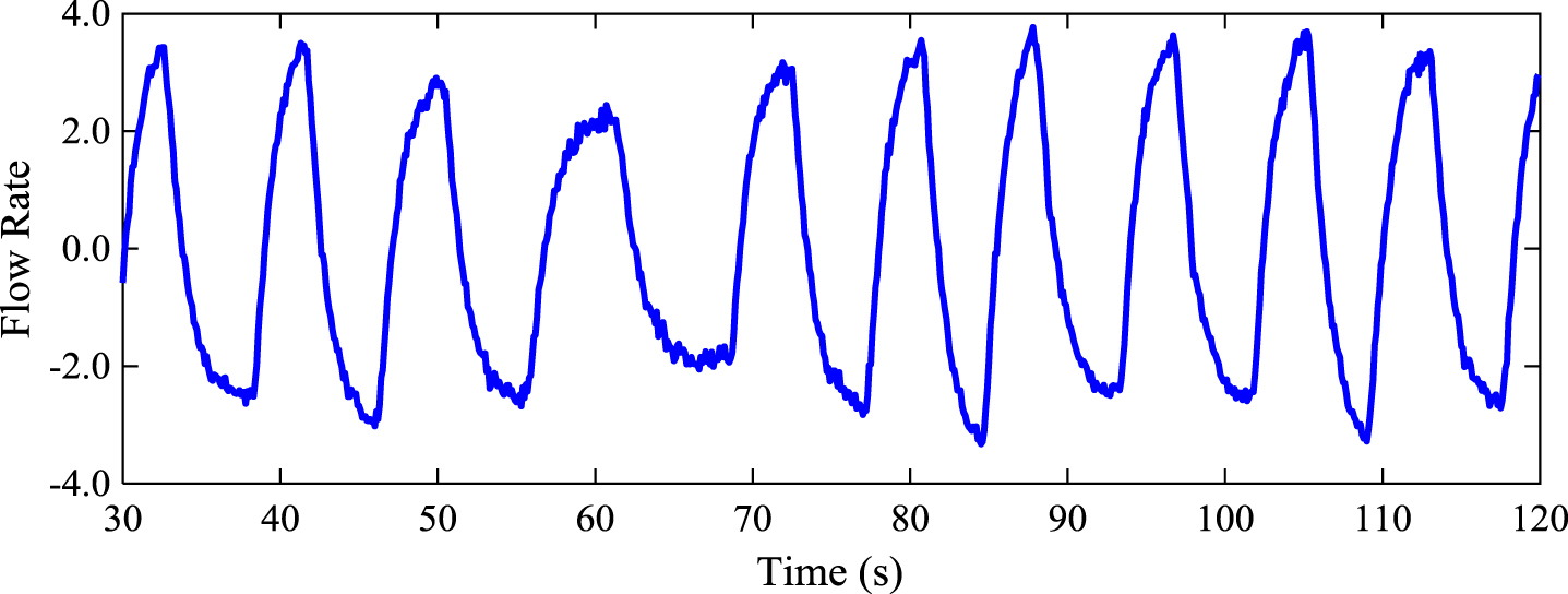
Error signal obtained from the flow process plant.

Table 4

Comparison result with EMD for real plant data

Data	Methods	Oscillations	Oscillation frequency (Hz)
			F	STD
Real Plant	Proposed	Detected	0.122	3.069×10^–16
	EMD	Not Detected	–	–

5 Conclusion and future scope

A new algorithm based on Prony method of infinite impulse response filter design and deep neural network (DNN) was proposed to detect and quantify the oscillations in control loop data. The proposed algorithm was successfully able to detect single, multiple and non-stationary control loop oscillations. In order to show the effectiveness of proposed algorithm, several simulation examples with and without noise were considered. Comparative study between DNN and other AI technique support vector machine (SVM) shows that DNN noise performance is better than SVM. Proposed method was also compared with the empirical mode decomposition (EMD) based method for oscillation detection speed and accuracy in estimating the amplitude and frequency of oscillations. Proposed scheme was found to be more accurate and faster than the EMD based approach. Further, real world applicability of proposed method was ascertained by using this method for oscillation detection in laboratory scaled flow process data. Comparison with the EMD based approach shows that the proposed algorithm is superior in oscillation detection and frequency estimation when applied on real world data. In future work, this algorithm will be implemented on real time hardware with the help of digital processors.

References

Mishra

, Kumar

and Rana

K.P.S.

, A Novel Intelligent Controller to Combat Stiction in Pneumatic Control Valve, Control Engineering Practice 33 (2014), 94–104. (DOI: https://doi.org/10.1016/j.conengprac.2014.09.001).

Mishra

, Kumar

and Rana

K.P.S.

, An online tuned novel nonlinear PI controller for stiction compensation in pneumatic control valves, ISA Transactions 58 (2015), 434–445. (DOI: https://doi.org/10.1016/j.isatra.2015.05.005).

Mishra

, Kumar

and Rana

K.P.S.

, Intelligent ratio control in presence of pneumatic control valve stiction, Arabian Journal for Science and Engineering 42(2) (2016), 677–689. (DOI: https://doi.org/10.1007/s13369-015-1853-0).

Sharma

, Kumar

and Rana

K.P.S.

, Pneumatic Control Valve Stiction Modelling Using Artificial Neural Network, in the Proceedings of International Conference on Emerging Trends in Computing and Communication Technologies (GEHU-2017), (2017), Dehradun, 1–6, November 17–18. (DOI: 10.1109/ICETCCT.2017.8280316).

Sharma

, Kumar

and Rana

K.P.S.

, Oscillation detection in control loops using PRONY analysis, in Proceedings of IEEE International conference on Computational and Characterization Techniques in Engineering and Science (CCTES-2018), (2018), Lucknow, India, September 14–15. (DOI: 10.1109/CCTES.2018.8674116).

Jelali

and Huang

, Detection and diagnosis of stiction in control loops, Springer, London, chapter 4, 2009. (DOI: 10.1007/978-1-84882-775-2).

, Wang

, Huang

and Lu

, The DCT-based oscillation detection method for a single time series, Journal of Process Control 20 (2010), 609–617. (DOI: 10.1016/j.jprocont.2010.02.012).

Sivalingam

and Hovd

, Use of cross wavelet transform for diagnosis of oscillations due to multiple sources, in Proceedings of 18th International Conference on Process control (2011), Tatranska Lomnica, Slovakia, June 14–17 (web: https://www.tib.eu/en/search/id/tema%3ATEMA20110800128/Use-of-cross-wavelet-transform-for-diagnosis-of/).

Srinivasan

and Rengaswamy

, Automatic oscillation detection and characterization in closed-loop systems, Control Engineering Practice 20 (2012), 733–746. (DOI: https://doi.org/10.1016/j.conengprac.2012.02.008).

10.

Wang

, Huang

and Lu

, Improved DCT-based method for online detection of oscillations in univariate time series, Control Engineering Practice 21 (2013), 622–630. (DOI: https://doi.org/10.1016/j.conengprac.2012.12.007).

11.

Naghoosi

and Huang

, Automatic detection and frequency estimation of oscillatory variables in the presence of multiple oscillations, Industrial & Engineering Chemistry Research 53 (2014), 9427–9438. (DOI: https://doi.org/10.1021/ie4037998).

12.

Guo

, Xie

, Horch

, Wang

, Su

and Wang

, Automatic detection of non-stationary multiple oscillations by an improved wavelet packet transform, Industrial and Engineering Chemical Research 53(40) (2014), 15686–15697. (DOI: https://doi.org/10.1021/ie502129c).

13.

Wardana

A.N.I.

, A method for detecting oscillation in control loops based on variational mode decomposition, in Proceedings of 2015 International Conference on Computer, Control, Informatics and Its Applications, (2015) Indonesia, 181–186. (DOI: 10.1109/IC3INA.2015.7377769).

14.

Xun

, Lei

, Yating

and Hongye

, Automatic oscillation detection based on Improved local mean decomposition, in Proceedings of the 35^th Chinese Control Conference (2016), China, 6766–6771. (DOI: 10.1109/ChiCC.2016.7554423).

15.

Xie

, Lang

, Horch

and Yang

, Online oscillation detection in the presence of signal intermittency, Control Engineering Practice 55 (2016), 91–100. (DOI: https://doi.org/10.1016/j.conengprac.2016.06.020).

16.

Yan

, Chen

and Zhang

, Using hidden markov model to identify oscillation temporal pattern for control loops, Chemical Engineering Research and Design 119 (2017), 117–129. (DOI: https://doi.org/10.1016/j.cherd.2017.01.011).

17.

Naghoosi

and Huang

, Wavelet transform based methodology for detection and characterization of multiple oscillations in nonstationary variables, Industrial and Engineering Chemical Research 56 (2017), 2083–2093. (DOI: https://doi.org/10.1021/acs.iecr.6b03075).

18.

Sharma

, Kumar

and Rana

K.P.S.

, Machine learning application for oscillation detection in control loops, in: Proc. Soft Computing: Theories & Applications (SoCTA-2018) (2018), NIT Jalandhar, Jalandhar, India, 1067–1075. (DOI: https://doi.org/10.1007/978-981-15-0751-9_98).

19.

Hauer

J.F.

, Demeure

C.J.

and Scharf

L.L.

, Initial results in Prony analysis of power system response signals,(, IEEE Transactions on Power Systems 5(1) (1990). (DOI: 10.1109/59.49090).

20.

Hauer

J.F.

, Application of prony analysis to the determination of modal content and equivalent model for measured power system response,(, Transactions on Power Systems 6(3) (1991). (DOI: 10.1109/59.119247).

21.

Parks

T.W.

and Burrus

C.S.

, Digital Signal Processing, New York, John Wiley & Sons, pp. 226–228, 1987.

22.

Sharma

, Kumar

and Rana

K.P.S.

, Automatic oscillation detection and quantification in process control loops using linear predictive coding, Engineering Science and Technology, an International Journal (JESTECH) 23(1) (2020), 123–143. (DOI: https://doi.org/10.1016/j.jestch.2019.04.006).

23.

Mitra

S.K.

, Digital signal processing: A computer based approach, McGraw Hill, 2^nd Edition, 2001.