Analysis of green supply chain considering green degree and sales effort with uncertain demand

Abstract

With resource exhaustion and environmental problems becoming more and more serious, green supply chain management attracts the attention of enterprises and scholars. For a new type of environmental-friendly product in this supply chain, we have no enough historical data to refer the demand. Hence, uncertainty theory is introduced as a tool to characterize the uncertainty of demand. Then this paper investigates the pricing, green degree and sales effort decisions in a green supply chain with a manufacturer and a retailer, where the demand of the product is described by uncertain variable. Considering the different power structures of supply chain, we build three expected value models and obtain equilibrium solutions, respectively. Then we analyze the influences of uncertain parameters and different power structures on decisions and profits. The results show that the green degree coefficient and sales effort coefficient have positive influences on the pricing, green degree and sales effort. Moreover, the results also show that decision leaders do not necessarily make more profits, which is up to the weights of green degree and sales effort. In addition, numerical analyses are given to show the correctness of results.

Keywords

Green supply chain management pricing decision uncertain demand uncertainty theory

1 Introduction

In recent years, the environmental problem have become increasingly prominent with the rapid development of economy. In order to cope with the environmental crisis, numerous countries and organizations have taken actions to realize the target of sustainable development, which aims to achieve the coordinated development of economy, society and environment. The United National Environment Programme has pointed out that the earth ecosystem and the sustainable development would be faced with great threats unless we take measures immediately [10]. Thus, the sustainable green supply chain management has attracted lots of attention of many scholars. The stages of green supply chain include raw materials procurement, green production, green marketing, green package, green consumption and reverse logistics, and the green production plays an important role in the decision-making process of supply chain [16]. The manufacture of green products can help enterprises to get competitive advantages in the market and establish a good image [29]. Generally, the green degree of products refers to the friendly degree of green products towards environment and is evaluated by the Analytic Hierarchy Process with respect to the economic, social and ecological indicators [2].

From the perspective of human beings, their environmental awareness is increasing under the environmental pressure. Consequently, consumers tend to buy environmental-friendly products, and they are willing to pay a premium for green products. In 2015, a market research firm GfK found that 80% of Chinese consumers claim that a brand or an enterprise should take responsibility for environment [9]. Another investigation indicated that more and more consumers show their environmental concern and desire to purchase green products [13]. Therefore, the influence of consumer’s environmental awareness on green production should not be ignored. While consumer’s environmental awareness does not always lead to the green purchasing behavior [28]. In this case, sales effort is an effective way to convert the environmental awareness into the purchase behavior [4], such as green advertising [8], that is, sales effort is an important factor in pricing decision.

In the past decades, the pricing decision problem of supply chain was studied widely. For instance, Liu et al. [20] investigated the impacts of consumer environmental awareness and competition level on the profits of channel members, and found that retailers’ profits increase with the intensification of production competition. Ghosh and Shah [6] analyzed the impact of cost-sharing contract on key decisions of supply chain players, and the result showed that cost-sharing contract is beneficial to manufacturers and supply chain’s performance. Pan et al. [24] studied different contract strategies under different power structures, and found that the revenue-sharing contract is beneficial to manufacturer under the manufacturer-dominant scenario. Basiri and Heydari [1] investigated the green channel coordination issue with substitutable products and proposed a collaboration model.

All the literatures mentioned above were studied in a certain situation. As we all know, there are many indeterministic phenomena in real life, and their influences on the decision-making process in supply chain can not be neglected. Some researches considered demand to be random and investigated multiple decision scenarios. For example, Mills [23] studied and compared the prices between certain and stochastic demand. Giri et al. [7] discussed the three-stage supply chain with random demand, which found that the repurchase contract is invalid in coordinating the supply chain. Hua and Li [11] introduced the sensitivity of the retailer’s order amount to manufacturer’s wholesale price, and developed a non-cooperative game model dominated by the retailer. They investigated two cooperative scenarios both with exogenous and endogenous retail-prices. Shi et al. [27] explored the influences of the different power structures on the performance of supply chain and the consumer welfare in stochastic environment. Xu et al. [30] studied a new income distribution mechanism for resource-based supply chain cooperation using the improved Shapley value method under random demand.

However, the premise of using probability theory is that the estimated cumulative probability distribution is close enough to the real frequency, which implies that we have to acquire a large number of effective data. Instead, the probability theory is invalid when historical data are lacking. For a new type of component, we may not precisely know its product quality and product life cycle. In this situation, we have to invite experts to give belief degrees to estimate the chance of event occurring. While Kahneman and Tversky [14] insisted that human beings usually overrate the impossible events. Liu [19] also pointed out that the gap between human estimation and real value is large. As a result, the belief degree should not be treated as a probability measure. In this situation, fuzzy set theory is an effective tool to handle this complicated nondeterministic environment. Many scholars have used triangular fuzzy random variable to describe the uncertainty factors. For instance, Zhao et al. [33] proposed a buyback contract model accounting for the fuzzy random demands with different risk attitudes. The results made clear that the model can allocate total benefits more fairly and keep the supply chain system stable by updating the buyback contract. Zhao and Wei [32] investigated the coordination of a two-echelon supply chain with fuzzy demand and developed two coordinating models based on symmetric information and asymmetric information about retailer’s scale parameter. Yang and Xiao [31] studied how channel leadership and governmental interventions influence prices, green levels and expected profits. Their investigation indicated that governmental interventions are not always beneficial to the green supply chain and the manufacturer.

When indeterminate phenomena behave neither randomness nor fuzziness, we need to find a new tool to deal with belief degree. Thus, Liu [17] introduced uncertainty theory in 2007, and characterized the belief degree by uncertain measure. Huang and Ke [12] firstly introduced uncertainty theory into the pricing decision problem of supply chain, in which the manufacturing cost, sales cost and demand are uncertain and described by uncertain variables. They studied the pricing strategies competitive manufacturers under different power structures. Further more, Chen et al. [3] regarded the retailer’s sales effort to be uncertain which depicted by an uncertain variable, and given a new form of sales effort cost. Afterwards, they discussed the influences of uncertain parameters on the pricing and sales effort decisions. Ke et al. [15] investigated the pricing decision problem in the case of manufacturer distributing products through traditional offline channel and e-commence online channel. Sang [25] studied the pricing and green degree decisions with a risk averse retailer in uncertain environment. The result showed that the manufacturer makes more profits when the retailer is more risk sensitive. Following that, Shen and Zhu [26] investigated the decision-making problem basing on the information about retailer’s scale parameter, and developed two coordination models with symmetric and asymmetric information.

Commonly, in many literatures, there are three power structures in two-stage supply chain: manufacturer-dominant game, retailer-dominant game and Nash game. Due to retailers power rising, such as Carrefour and JD, they own more power and even become a leader in the decision of supply chain [5]. The change of channel power structures has a significant impact on the decision level of supply chain [21]. Thus, we are interested in studying how supply chain make decisions under different structures. Combing through the previous literature, we found that no literature studied the pricing, green degree and sales effort decisions of a two-stage supply chain including a manufacturer and a retailer with uncertain demand under assumption that the coefficients of price, green degree and sales effort are simultaneously described by uncertain variables. Hence, we introduce uncertainty theory into the supply chain management in this case and explore the pricing, green degree and sales effort decisions of the two-stage supply chain. The wholesale price and green degree are determined by manufacturer, while the retail price and sales effort are determined by retailer. We build three models under different power structures: (1) integrated scenario, (2) manufacturer-dominant scenario, and (3) retailer-dominant scenario. Then we compare the decision level of each model, and discuss how power structures and uncertain parameters influences the performance of supply chain.

After analysis, the price parameter β has a negative impact on the optimal green degree, pricing and sales effort decisions, while the green degree parameter θ and sales effort parameter γ have positive impacts on the optimal green degree, pricing and sales effort decisions, respectively. Following that, we found that green degree and sales effort level are affected by the decision-making order and their ranking is related to the value of parameters. Finally, when manufacturer has high bargaining power in the supply chain, he does not necessarily benefit more from his high bargaining power. Therefore, in some cases, it is better for manufacturer to abandon the dominance. The rest of the paper is organized as follows. In section 2, some important definitions and theorems of uncertainty theory are introduced. Section 3 proposes the notations and assumptions for the models. In section 4, we build three models and obtain the equilibrium solutions. In addition, the solutions are compared for the analysis of chain’s performances in three models. Section 5 offers numerical experiment to verify the correctness of the result and analyze the sensitivity of parameters. In section 6, the conclusion is given.

2 Preliminaries

Uncertainty theory was found by Liu [17] in 2007 which is a branch of axiomatic mathematics for modeling human uncertainty. Some important definitions and theorems of uncertainty theory are introduced in the following to solve pricing issue in our study.

Let Γ be a nonempty set, and let ℒ be a σ-algebra over Γ. Each element Λ in ℒ is called an event.

Definition 1. ([17]) An uncertain measure ℳ on ℒ is defined by the following axioms: Axiom 1. (Normality Axiom) ℳ {Γ} =1 for the universal set Γ; Axiom 2. (Duality Axiom) ℳ {Λ} + ℳ {Λ^c} =1 for any event Λ; Axiom 3. (Subadditivity Axiom) For every countable sequence of events Λ₁, Λ₂, ⋯, we have $ℳ {⋃_{i = 1}^{\infty} Λ_{i}} \leq \sum_{i = 1}^{\infty} ℳ {Λ_{i}} .$ (1)

The triplet (Γ, ℒ, ℳ) is called an uncertainty space. Furthermore, a product uncertain measure was defined by Liu [17]: Axiom 4. (Product Axiom) Let (Γ_k, ℒ_k, _ℳk) be uncertainty spaces, k = 1, 2, ⋯. If a product uncertain measure ℳ satisfies $ℳ {\prod_{k = 1}^{\infty} Λ_{k}} = ⋀_{k = 1}^{\infty} ℳ_{k} {Λ_{k}}$ (2) where Λ_k are arbitrarily chosen from ℒ_k, k = 1, 2, ⋯, respectively. Then ℳ is called an uncertain measure.

Definition 2. ([17]) Suppose that a function ξ from an uncertainty space (Γ, ℒ, ℳ) to the set of real numbers such that {ξ ∈ B} is an event for any Borel set B of real numbers. Then we call ξ an uncertain variable.

Definition 3. ([17]) Let ξ be an uncertain variable. The uncertainty distribution Φ of ξ is $Φ (x) = ℳ {ξ \leq x}$ (3) for any real number x.

Definition 4. ([18]) Assume that an uncertainty distribution Φ (x) is a continuous and strictly increasing function in x at which 0 < Φ (x) <1, and $lim_{x \to - \infty} Φ (x) = 0, lim_{x \to + \infty} Φ (x) = 1 .$ (4) Then Φ (x) is regarded to be regular.

Definition 5. ([18]) Let ξ be an uncertain variable whose uncertainty distribution Φ (x) is regular. Then the inverse function Φ^-1 (α) is called the inverse uncertainty distribution of ξ.

Definition 6. ([18]) Let ξ₁, ξ₂, ⋯ , ξ_n be uncertain variables. If $ℳ {⋂_{i = 1}^{n} (ξ_{i} \in B_{i})} = ⋀_{i = 1}^{n} ℳ {ξ_{i} \in B_{i}}$ (5) holds for any Borel sets B₁, B₂, ⋯ , B_n of real numbers, then ξ₁, ξ₂, ⋯ , ξ_n are said to be independent.

Definition 7. ([17]) Let ξ be an uncertain variable. The expected value of ξ is defined by $E [ξ] = \int_{0}^{+ \infty} ℳ {ξ \geq x} dx - \int_{- \infty}^{0} ℳ {ξ \leq x} dx,$ (6) provided that at least one of the two integrals is finite.

Theorem 1. ([18]) Let ξ be an uncertain variable with regular uncertain distribution Φ. Then the expectation of ξ is $E [ξ] = \int_{- \infty}^{+ \infty} x dΦ (x) = \int_{0}^{1} Φ^{- 1} (α) dα$ (7)

Theorem 2. ([18]) Let ξ and η be independent uncertain variables with finite expected values, and let a and b be arbitrary real numbers. Then we have $E [a ξ + b η] = aE [ξ] + bE [η] .$ (8)

3 Problem description

We consider a supply chain with a manufacturer and a retailer, where the manufacturer pays investment in the green degree of products and distributes green products to the retailer, then the retailer sells green products to final consumers by making sales effort. The green degree and the wholesale price are determined by manufacturer. The sales effort and the retail price are determined by retailer.

The customer demand function D can be expressed as follows: $D = a - β p + θ e + γ s .$ (9)

This linear form of demand function could be found in [22]. Here, a is the total market potential, p is the retail price, e is the green degree of products, and s is the retailer’s sales effort. Let β, θ and γ represent retail price coefficient, green degree coefficient and sales effort coefficient, respectively. Considering a new product lack of historical data, we suppose that β, θ and γ are independent nonnegative uncertain variables with regular uncertainty distributions Φ₁, Φ₂, Φ₃, respectively. Moreover, the expectation of β, θ and γ exist. Similar to the Reference [25], the greening investment cost is written by $\frac{1}{2} {he}^{2}$ , where h is the greening investment cost coefficient. The sales effort of retailer is given by $\frac{1}{2} {ks}^{2}$ , where k is the sales efforts investment cost coefficient. Such a cost function is used repeatedly in the Reference [1].

According to the above assumptions, the manufacturer’s profit function is formulated as $π_{m} = (w - c) (a - β p + θ e + γ s) - \frac{1}{2} {he}^{2},$ (10) and the retailer’s profit function is $π_{r} = (p - w) (a - β p + θ e + γ s) - \frac{1}{2} {ks}^{2} .$ (11)

The channel profit function can be written as $π_{sc} = (p - c) (a - β p + θ e + γ s) - \frac{1}{2} {he}^{2} - \frac{1}{2} {ks}^{2} .$ (12)

To keep the supply chain profitable, the customer demand of green product should be nonnegative, and the retail price should be larger than marginal manufacturing cost. That is, a - βp + θe + γs > 0 and p > w > c.

4 Modeling and comparison

In this section, we establish three models under integrated scenario, manufacturer-dominant scenario and retailer-dominant scenario, and derive the equilibrium solutions. Then we compare the performances of supply chain in these three models.

4.1 Integrated scenario

Under the integrated scenario, the manufacturer and the retailer form an ideal organization and make decisions together to maximizing the total expected channel profit. The decision model under the integrated scenario is a single-level programming model, which can be built as following format:

$\begin{matrix} \max_{(p, s, e)} E [π_{sc}^{I} (p, s, e)] \\ = E [(p - c) (a - β p + θ e + γ s) - \frac{1}{2} {he}^{2} - \frac{1}{2} {ks}^{2}] \\ = (p - c) (a - pE [β] + eE [θ] + sE [γ]) - \frac{1}{2} {he}^{2} - \frac{1}{2} {ks}^{2} . \end{matrix}$

Proposition 1. Under the integrated scenario, the expected channel profit is jointly concaved with respect to p, e, and s, if 2hE [β] - E² > 0 and 2hkE [β] - kE² [θ]) - hE² [γ] >0. Under the above conditions, the optimal retail price, green degree and sales effort can be derived as follows:

$p_{sc}^{I *} = \frac{c ({kE}^{2} [θ] + {hE}^{2} [γ]) - hk (a + cE [β])}{- 2 hkE [β] + {hE}^{2} [γ] + {kE}^{2} [θ]}$ ,

$e_{sc}^{I *} = \frac{- kE [θ] (a - cE [β])}{- 2 hkE [β] + {hE}^{2} [γ] + {kE}^{2} [θ]}$ ,

$s_{sc}^{I *} = \frac{- hE [γ] (a - cE [β])}{- 2 hkE [β] + {hE}^{2} [γ] + {kE}^{2} [θ]}$ .

Then the optimal expected channel profit $E^{*} [π_{sc}^{I}]$ is

$E^{*} [π_{sc}^{I}] = \frac{- kh (a - cE [β])^{2}}{2 (- 2 hkE [β] + {hE}^{2} [γ] + {kE}^{2} [θ])}$ .

Proposition 1 is verified in Appendix.

4.2 Manufacturer-dominant scenario

Under the manufacturer-dominant scenario, the manufacturer and the retailer make their decisions alone in order to achieve their own maximal expected profits. It is a bi-level programming problem, in which the manufacturer decides the wholesale price and green degree first, and then the retailer decides the retail price and sales effort. The expected value model can be formulated as follows:

${\begin{matrix} \max_{(w, e)} E [π_{m}^{ℳ} (w, e, p^{*}, s^{*})] \\ s . t . where p^{*} and s^{*} are derived from solving \\ the following problem \\ \max_{(p, s)} E [π_{r}^{ℳ} (p, s)] \end{matrix} .$

Proposition 2. Under the manufacturer-dominant scenario, the expected profit of manufacturer $E [π_{m}^{ℳ}]$ is jointly concave with respect to w and e, if kE² [θ] +2hE² [γ] -4khE [β] <0. Under the above conditions, the optimal wholesale price and green degree can be obtained as follows:

$w^{ℳ *} = \frac{ckE [β] E^{2} [θ] - h (a + cE [β]) (2 kE [β] - E^{2} [γ])}{E [β] (- 4 hkE [β] + 2 {hE}^{2} [γ] + {kE}^{2} [θ])}$ ,

$e^{ℳ *} = \frac{kE [θ] (a - cE [β])}{- 4 hkE [β] + 2 {hE}^{2} [γ] + {kE}^{2} [θ]}$ .

The optimal expected profit of manufacturer is

$E^{*} [π_{m}^{ℳ}] = \frac{- hk (a - cE [β])^{2}}{2 (- 4 hkE [β] + 2 {hE}^{2} [γ] + {kE}^{2} [θ])}$ .

Proposition 2 is proved in Appendix.

Proposition 3. Under the manufacturer-dominant scenario, the expected profit of retailer $E [π_{r}^{ℳ}]$ is jointly concaved in p and s, if 2kE [β] - E² [γ] >0. Under the above conditions, the optimal retail price and sales effort can be summed as follows:

$p^{ℳ *} = \frac{h (a + cE [β]) (E^{2} [γ] - kE [β]) + kE [β] ({cE}^{2} [θ] - 2 ah)}{E [β] (- 4 hkE [β] + 2 {hE}^{2} [γ] + {kE}^{2} [θ])}$ ,

$s^{ℳ *} = \frac{- hE [γ] (a - cE [β])}{- 4 hkE [β] + 2 {hE}^{2} [γ] + {kE}^{2} [θ]}$ .

The optimal expected profit of retailer is

$E^{*} [π_{r}^{ℳ}] = \frac{h^{2} k (a - cE [β])^{2} (2 kE [β] - E^{2} [γ])}{2 (- 4 hkE [β] + 2 {hE}^{2} [γ] + {kE}^{2} [θ])}$ .

Then the optimal expected channel profit is

$E^{*} [π_{sc}^{ℳ}] = \frac{(a - cE [β]) [{kE}^{2} [θ] - 3 h (2 kE [β] - E^{2} [γ])]}{2 (- 4 hkE [β] + 2 {hE}^{2} [γ] + {kE}^{2} [θ])}$ .

Proposition 3 is shown in Appendix.

4.3 Retailer-dominant scenario

Under the retailer-dominant scenario, the manufacturer and the retailer make their decisions alone in order to achieve their own maximal expected profits. It is a bi-level programming problem, in which the retailer decides the retail price and sales effort first, then the manufacturer decides the wholesale price and green degree. The expected value model can be formulated as follows:

${\begin{matrix} \max_{(p, s)} E [π_{r}^{R} (w^{*}, e^{*}, p, s)] \\ s . t . where w^{*} and e^{*} are derived from solving \\ the following problem \\ \max_{(w, e)} E [π_{m}^{R} (w, e)] \end{matrix} .$

Proposition 4. Under the retailer-dominant scenario, the expected profit of manufacturer $E [π_{m}^{R}]$ is jointly concave with respect to w and e, if 2kE [β] - E² [γ] >0. Under the above conditions, the optimal wholesale price and green degree are obtained as follows:

$w^{R *} = \frac{- 3 chkE [β] + {chE}^{2} [γ] + 2 {ckE}^{2} [γ] - ahk}{- 4 hkE [β] + {hE}^{2} [γ] + 2 {kE}^{2} [θ]}$ ,

$e^{R *} = \frac{- kE [θ] (a - cE [β])}{- 4 hkE [β] + {hE}^{2} [γ] + 2 {kE}^{2} [θ]}$ .

Hence, the optimal profit of manufacturer is

$E^{*} [π_{m}^{R}] = \frac{{hk}^{2} (a - cE [β])^{2} (2 hE [β] - E^{2} [θ])}{(- 4 hkE [β] + {hE}^{2} [γ] + 2 {kE}^{2} [θ])^{2}}$ .

The proof of Proposition 4 is in Appendix.

Proposition 5. Under the retailer-dominant scenario, the expected profit of retailer $E [π_{r}^{R}]$ is jointly concave with respect to p and s, if 4hkE [β] - hE² [γ] -2kE² [θ] >0. Under the above conditions, the optimal retail price and sales effort are obtained as follows:

$p^{R *} = \frac{- {chkE}^{2} [β] + chE [β] E^{2} [γ] + ckE [β] E^{2} [θ] - 3 ahkE [β] + {akE}^{2} [θ]}{E [β] (- 4 hkE [β] + {hE}^{2} [γ] + 2 {kE}^{2} [θ])}$ ,

$s^{R *} = \frac{- hE [γ] (a - cE [β])}{- 4 hkE [β] + {hE}^{2} [γ] + 2 {kE}^{2} [θ]}$ .

The optimal expected profit of retailer is

$E^{*} [π_{r}^{R}] = \frac{- hk (a - cE [β])^{2}}{2 (- 4 hkE [β] + {hE}^{2} [γ] + 2 {kE}^{2} [θ])}$ .

Thus, the optimal expected channel profit is

$E^{*} [π_{sc}^{R}] = \frac{hk (a - cE [β])^{2} (6 hkE [β] - {hE}^{2} [γ] - 3 {kE}^{2} [θ])^{2})}{2 (- 4 hkE [β] + {hE}^{2} [γ] + 2 {kE}^{2} [θ])^{2}}$ .

Proposition 5 is proved in Appendix.

4.4 Discussion

In this subsection, we investigate the impacts of parameters, and compare the performances of green supply chain in the above three models. After that, some corollaries are obtained.

Corollary 1. In three models, when 2hE [β] - E² [θ] >0 and 2hkE [β] - kE² [θ] - hE² [γ] >0, we have the following results:

(1) The optimal green degree, retail price, sales effort and expected channel profit rise when E [θ] increases.

(2) The optimal green degree, retail price, sales effort and expected channel profit rise when E [γ] increases.

The result of Corollary 1 indicates that the optimal green degree, retail price and expected channel profit increase with the rise of E [θ]. The manufacturer would be encouraged to invest more in the improvement of green degree for products when E [θ] rises because the demand is positively related to E [θ]. Following that, the retailer will make more sales efforts for green products. Consequently, the demand and the expected channel profit will grow. However, more greening investments mean higher manufacturing costs, which brings higher retail prices. In this situation, consumers have to pay more for green products. Similarly, the optimal green degree, retail price and expected channel profit increase with the rise of E [γ]. Due to the demand being positively related to E [γ], the demand will improve with E [γ] increasing, which inspires the retailer to make more sales efforts for green product. Affected by the retailer behavior, the manufacturer will invest more in the improvement of green degree, then the demand and expected channel profit will augment. More investments to sales effort mean higher costs, so the retail price will grow.

Corollary 2. For the optimal green degree, sales effort and expected channel profit in three models, we have the following orders:

(1) If hE² [γ] > kE² [θ], then e^I∗ > e^ℳ∗ > e^R∗, s^I∗ > s^ℳ∗ > s^R∗ and $E^{*} [π_{sc}^{I}] > E^{*} [π_{sc}^{ℳ}] > E^{*} [π_{sc}^{R}]$ .

(2) If hE² [γ] = kE² [θ], then e^I∗ > e^ℳ∗ = e^R∗, s^I∗ > s^ℳ∗ = s^R∗ and $E^{*} [π_{sc}^{I}] > E^{*} [π_{sc}^{ℳ}] = E^{*} [π_{sc}^{R}]$ .

(3) If hE² [γ] < kE² [θ], then e^I∗ > e^R∗ > e^ℳ∗, s^I∗ > s^R∗ > s^ℳ∗ and $E^{*} [π_{sc}^{I}] > E^{*} [π_{sc}^{R}] > E^{*} [π_{sc}^{ℳ}]$ .

Corollary 2 shows that the optimal green degree, the sales effort and the expected channel profit are greatest in integrated scenario. It means that the integrated decision is more environmental-friendly and profitable than that in other scenarios. So the collaboration of chain members can help chain to improve environmental performance significantly and boost more profits.

Corollary 3. The optimal retail price in three models has the following orders:

(1) If hE² [γ] = kE² [θ] and $\frac{E^{2} [γ]}{k} < E [β] < \frac{2 E^{2} [γ]}{k}$ , then p^I∗ > p^ℳ∗ = p^R∗.

(2) If hE² [γ] = kE² [θ] and $\frac{2 E^{2} [γ]}{k} < E [β] < \frac{a}{c}$ , then p^ℳ∗ = p^R∗ > p^I∗.

(3) If hE² [γ] > kE² [θ] and $\frac{E^{2} [γ]}{k} < E [β] < \frac{2 E^{2} [γ]}{k}$ , then p^I∗ > p^ℳ∗ > p^R∗.

(4) If hE² [γ] > kE² [θ] and $\frac{2 E^{2} [γ]}{k} < E [β] < \frac{a}{c}$ , then p^ℳ∗ > p^R∗ > p^I∗.

(5) If hE² [γ] < kE² [θ] and $\frac{E^{2} [γ]}{k} < E [β] < \frac{2 E^{2} [γ]}{k}$ , then p^I∗ > p^R∗ > p^ℳ∗.

(6) If hE² [γ] < kE² [θ] and $\frac{2 E^{2} [γ]}{k} < E [β] < \frac{a}{c}$ , then p^ℳ∗ > p^R∗ > p^I∗.

Corollary 3 indicates that when $\frac{E^{2} [γ]}{k} < E [β] < \frac{2 E^{2} [γ]}{k}$ , the optimal retail price is highest in integrated scenario. In this case, consumers need to pay more for high green degree products. When $\frac{2 E^{2} [γ]}{k} < E [β] < \frac{a}{c}$ , the optimal retail price is lowest in integrated scenario. This is favourable for consumers because they can enjoy products with high green degree and low price. When hE² [γ] = kE² [θ], the optimal retail price in retailer-dominant scenario is equal to that in manufacturer-dominant scenario. When hE² [γ] < kE² [θ], the optimal retail price in retailer-dominant scenario is higher than that in manufacturer-dominant scenario. When hE² [γ] > kE² [θ], the optimal retail price in manufacturer-dominant scenario is higher than that in retailer-dominant scenario.

Corollary 4. The expected profit of manufacturer in three models has the following relationships:

(1) If hE² [γ] > kE² [θ], then $E^{*} [π_{m}^{ℳ}] > E^{*} [π_{m}^{R}]$ .

(2) If hE² [γ] = kE² [θ], then $E^{*} [π_{m}^{ℳ}] = E^{*} [π_{m}^{R}]$ .

(3) If hE² [γ] < kE² [θ] and $\frac{E^{2} [γ]}{2 k} + \frac{E^{2} [θ]}{2 h} < E [β] < \frac{2 {hE}^{2} [γ] + 5 {kE}^{2} [θ] + \sqrt{k^{2} E^{4} [θ] - 4 h^{2} E^{4} [γ] + 4 {hkE}^{2} [θ] E^{2} [γ]}}{8 hk}$ , then $E^{*} [π_{m}^{R}] > E^{*} [π_{m}^{ℳ}]$ .

(4) If hE² [γ] < kE² [θ] and $\frac{2 {hE}^{2} [γ] + 5 {kE}^{2} [θ] + \sqrt{k^{2} E^{4} [θ] - 4 h^{2} E^{4} [γ] + 4 {hkE}^{2} [θ] E^{2} [γ]}}{8 hk} < E [β] < \frac{a}{c}$ , then $E^{*} [π_{m}^{ℳ}] > E^{*} [π_{m}^{R}]$ .

Corollary 4 implies that when hE² [γ] > kE² [θ], the expected profit of manufacturer is larger in manufacturer-dominant scenario than that in retailer-dominant scenario. When hE² [γ] = kE² [θ], the expected profit of manufacturer in manufacturer-dominant scenario is equal to that in retailer-dominant scenario. When hE² [γ] < kE² [θ], if E [β] satisfies $\frac{E^{2} [γ]}{2 k} + \frac{E^{2} [θ]}{2 h} < E [β] < \frac{2 {hE}^{2} [γ] + 5 {kE}^{2} [θ] + \sqrt{k^{2} E^{4} [θ] - 4 h^{2} E^{4} [γ] + 4 {hkE}^{2} [θ] E^{2} [γ]}}{8 hk}$ , then the expected profit of manufacturer is larger in retailer-dominant scenario than that in manufacturer-dominant scenario. If $\frac{2 {hE}^{2} [γ] + 5 {kE}^{2} [θ] + \sqrt{k^{2} E^{4} [θ] - 4 h^{2} E^{4} [γ] + 4 {hkE}^{2} [θ] E^{2} [γ]}}{8 hk} < E [β] < \frac{a}{c}$ , then the expected profit of manufacturer is larger in manufacturer-dominant scenario than that in retailer-dominant scenario.

Corollary 5. The expected profit of retailer in three models has the following relationships:

(1) If hE² [γ] > kE² [θ] and $\frac{E^{2} [γ]}{2 k} + \frac{E^{2} [θ]}{2 h} < E [β] < \frac{5 {hE}^{2} [γ] + 2 {kE}^{2} [θ] + \sqrt{h^{2} E^{4} [γ] - 4 k^{2} E^{4} [θ] + 4 {hkE}^{2} [θ] E^{2} [γ]}}{8 hk}$ , then $E^{*} [π_{r}^{ℳ}] > E^{*} [π_{r}^{R}]$ .

(2) If hE² [γ] > kE² [θ] and $\frac{5 {hE}^{2} [γ] + 2 {kE}^{2} [θ] + \sqrt{h^{2} E^{4} [γ] - 4 k^{2} E^{4} [θ] + 4 {hkE}^{2} [θ] E^{2} [γ]}}{8 hk} < E [β] < \frac{a}{c}$ , then $E^{*} [π_{r}^{R}] > E^{*} [π_{r}^{ℳ}]$ .

(3) If hE² [γ] = kE² [θ], then $E^{*} [π_{r}^{ℳ}] = E^{*} [π_{r}^{R}]$ .

(4) If hE² [γ] < kE² [θ], then $E^{*} [π_{r}^{R}] > E^{*} [π_{r}^{ℳ}]$ .

Corollary 5 shows that when hE² [γ] > kE² [θ], if E [β] satisfies the condition $\frac{E^{2} [γ]}{2 k} + \frac{E^{2} [θ]}{2 h} < E [β] < \frac{5 {hE}^{2} [γ] + 2 {kE}^{2} [θ] + \sqrt{h^{2} E^{4} [γ] - 4 k^{2} E^{4} [θ] + 4 {hkE}^{2} [θ] E^{2} [γ]}}{8 hk}$ , the expected profit of retailer is larger in manufacturer-dominant scenario than that in retailer-dominant scenario. If E [β] satisfies $\frac{5 {hE}^{2} [γ] + 2 {kE}^{2} [θ] + \sqrt{h^{2} E^{4} [γ] - 4 k^{2} E^{4} [θ] + 4 {hkE}^{2} [θ] E^{2} [γ]}}{8 hk} < E [β] < \frac{a}{c}$ , then the expected profit of retailer in retailer-dominant scenario than that in manufacturer-dominant scenario. When hE² [γ] = kE² [θ], the expected profit of retailer in manufacturer-dominant scenario is equal to that in retailer-dominant scenario. When hE² [γ] < kE² [θ], the expected profit of retailer in retailer-dominant scenario than that in manufacturer-dominant scenario.

The proof of all corollaries above are shown in Appendix.

5 Numerical analyses

5.1 Numerical experiment

In this section, we employ a numerical example to illustrate the effectiveness of the proposed method. According to the Reference [3] and the assumptions mentioned above, Table 2 shows the basic parameters. By Theorem 1, we have $E [β] = \int_{0}^{1} 2 + (6 - 2) α dα = 4,$ $E [θ] = \int_{0}^{1} 1 + (3 - 1) α dα = 1,$ $E [γ] = \int_{0}^{1} 2 α dα = 2 .$

Table 1
Notations

Symbol Meaning

a the total market potential

β the retail price coefficient of customer demand

θ the green degree coefficient of customer demand

γ the sales effort coefficient of customer demand

p the retail price

s the green sales effort

e the green degree of product

c the unit manufacturing cost

w the wholesale price

h the greening investment coefficient

k the sales efforts investment coefficient

π _m the manufacturer’s profit

π _r the retailer’s profit

π _sc the channel profit

Symbol	Meaning
a	the total market potential
β	the retail price coefficient of customer demand
θ	the green degree coefficient of customer demand
γ	the sales effort coefficient of customer demand
p	the retail price
s	the green sales effort
e	the green degree of product
c	the unit manufacturing cost
w	the wholesale price
h	the greening investment coefficient
k	the sales efforts investment coefficient
π _m	the manufacturer’s profit
π _r	the retailer’s profit
π _sc	the channel profit

Table 2

The value of parameters

parameter	value	parameter	value
a	150	h	1
c	15	k	1
β	ℒ (2, 6)	θ	ℒ (0, 2)
γ	ℒ (1, 3)

Substituting the above values in Table 2 into the corresponding parameters, we derive the optimal decisions and profits under different structures shown in Table 3.

Table 3

The optimal decisions

	w	e	p	s	E [π_m]	E [π_r]	E [π_sc]
I		30	45	60			1350
ℳ	27.86	12.86	40.71	25.71	578.57	330.61	8909.18
R	20	9	39.75	18	283.5	405	688.5

From Table 3, we come to the conclusion that the green degree, the sales effort and the expected channel profit are highest in integrated scenario. It means that the economic performance and environmental performance of supply chain are greatest in the integrated scenario. Thus, the integrated decision-making should be taken in supply chain for the coordinated development of economy and environment, which is consistent with Corollary 2. Another conclusion is that the dominated enterprise can get more profits in this situation. Therefore, the manufacturer and the retailer will fight for the decision-making dominance. These are consistent with the previous results and corollaries.

5.2 Sensitivity of θ

In this subsection, we analyze the influence of parameter θ on the green degree, sales effort, retail price, expected profit of manufacturer, expected profit of retailer and expected channel profit in three models. The remaining parameters are assumed as follows: a = 150, c = 15, h = 1, k = 1, β = ℒ (7, 9) , γ = ℒ (1, 3).

As shown in Figure 1, the green degree in these three scenarios is rising with the increase of E [θ]. The green degree in integrated scenario is always higher than that in other two scenarios. The green degree in manufacturer-dominant scenario is higher than that in retailer-dominant scenario when E [θ] is small enough, and the difference of green degree narrows between two decentralized scenarios. When E [θ] is greater than a threshold in Corollary 2, the green degree in retailer-dominant scenario is higher than that in manufacturer-dominant scenario. From Figure 2 and Figure 4, we can draw the similar conclusions, the sales efforts and the expected channel profits are climbing with the increase of E [θ] in three scenarios. The results above are in line with the common sense.

Fig. 1

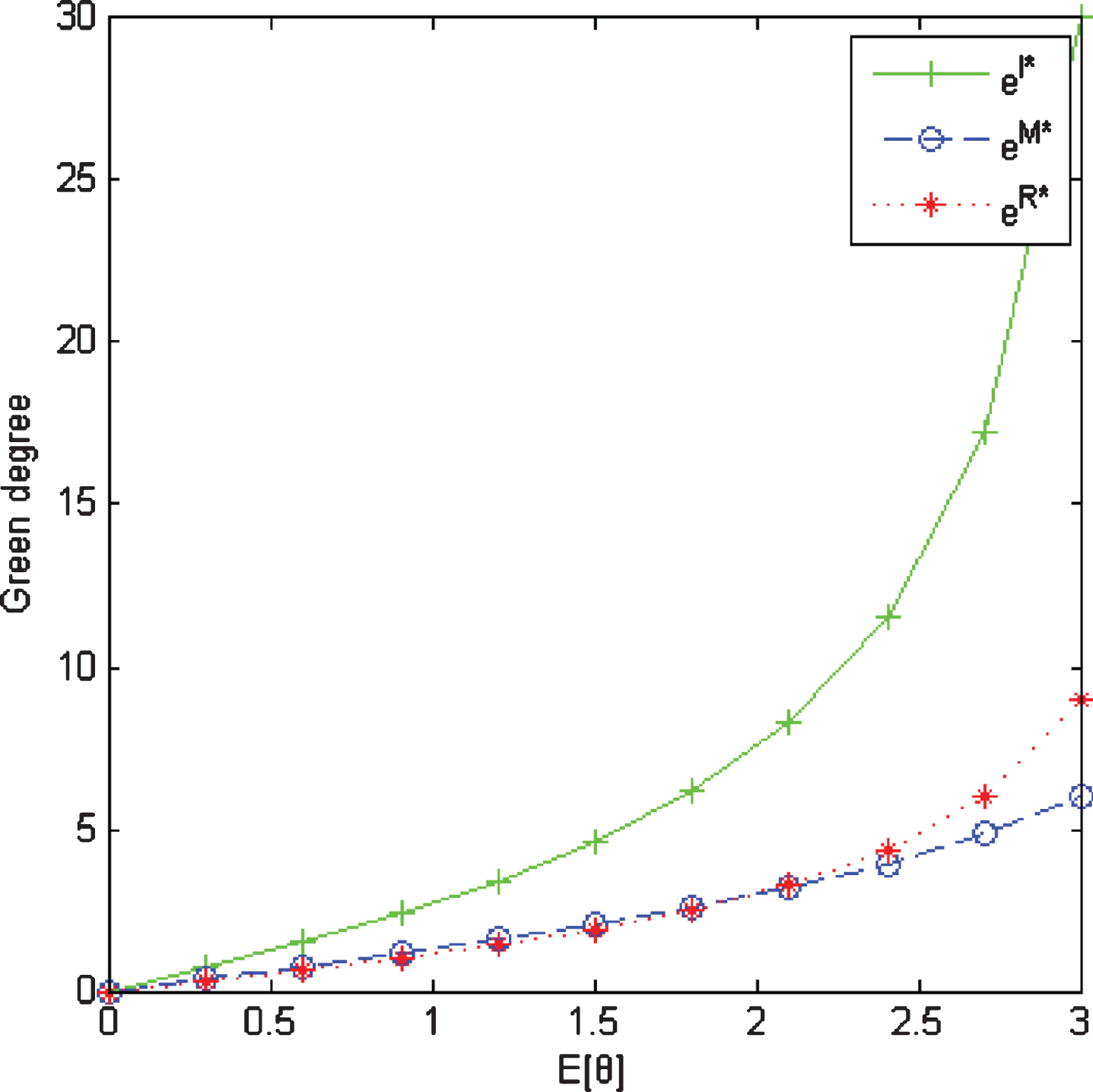
The effect of E [θ] on green degree.

Fig. 2

The effect of E [θ] on sales effort.

Fig. 3

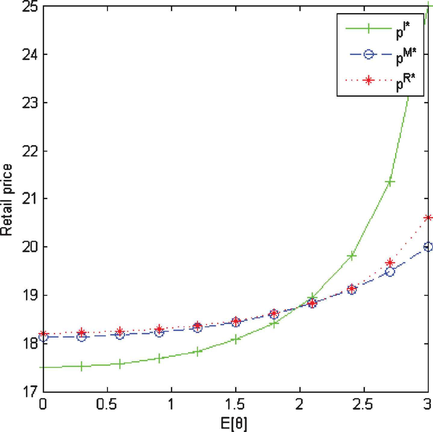
The effect of E [θ] on retail price.

Fig. 4

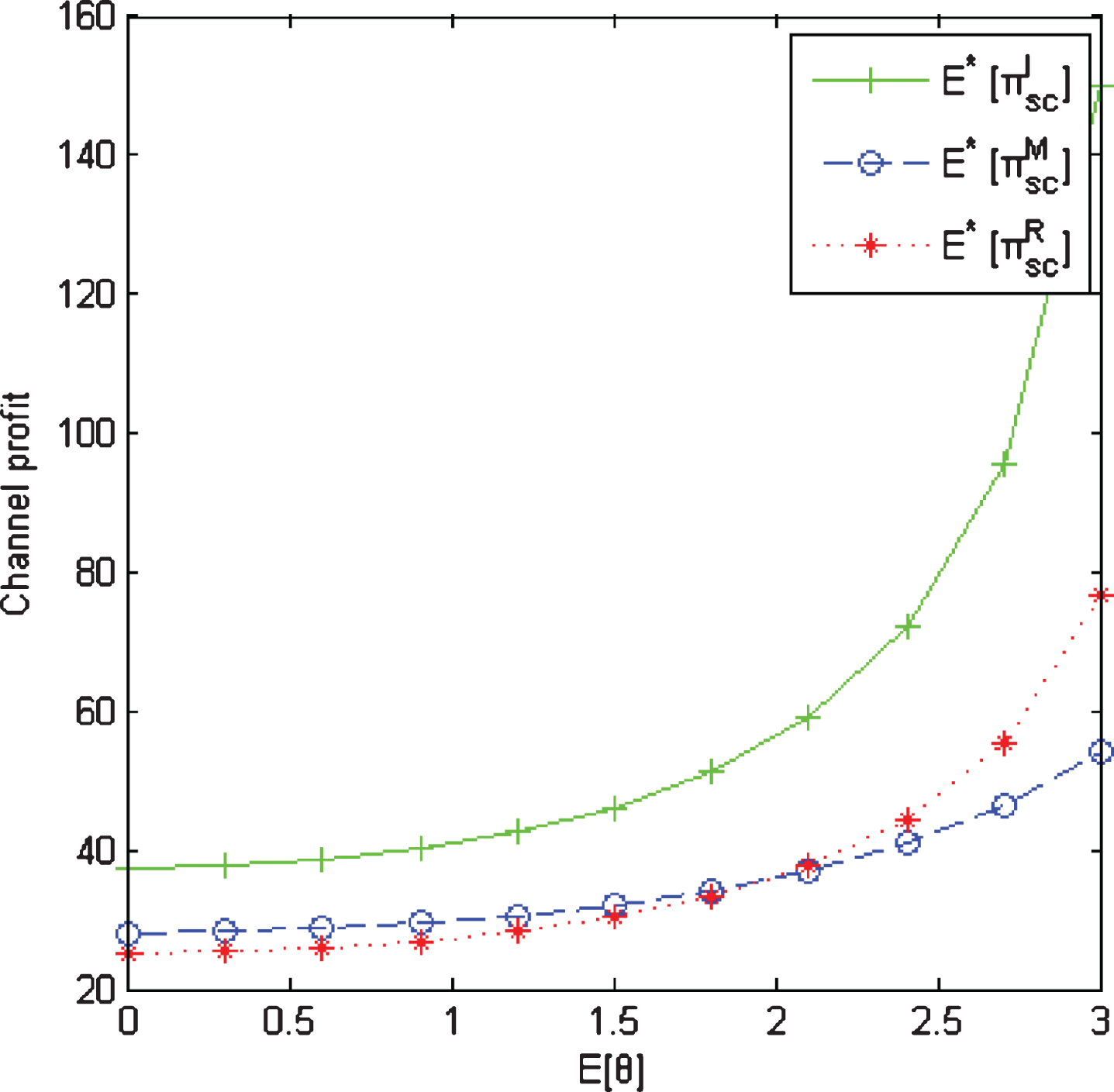
The effect of E [θ] on the expected channel profit.

As shown in Figure 3, when E [θ] increases, the retail price rises in these three scenarios because the greening investment increases concerning E [θ] leading to high cost. The retail price is highest in retailer-dominant scenario and lowest in integrated scenario when E [θ] is small enough. As E [θ] increases, the difference of green degree in three scenarios decreases. When E [θ] is larger than a threshold in Corollary 2, the retail price in integrated scenario is higher than that in other two scenarios.

As shown in Figure 5, the expected profit of manufacturer expands when E [θ] increases in manufacturer-dominant scenario and retailer-dominant scenario because the rise of E [θ] can bring about an improvement of demand. As E [θ] grows, the order of the expected profit of manufacturer in such two scenarios is changing. Similarly, the comparison of the expected profit of retailer in such two models shown in Figure 6, it claims that the expected profit of retailer increases with the rise of E [θ] in such two scenarios and is larger in retailer-dominant scenario than that in manufacturer-dominant scenario.

Fig. 5

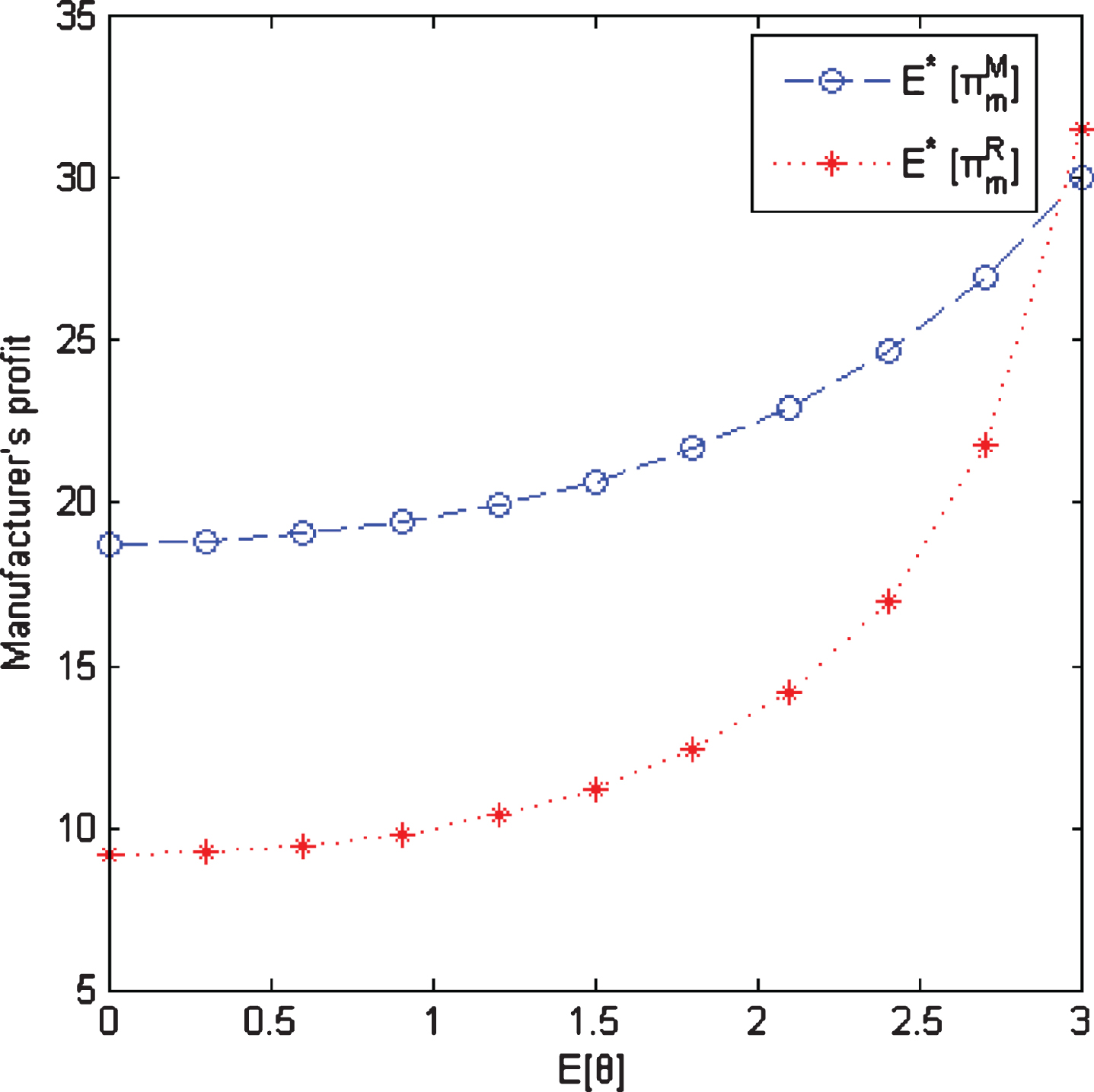
The effect of E [θ] on the expected profit of manufacturer.

Fig. 6

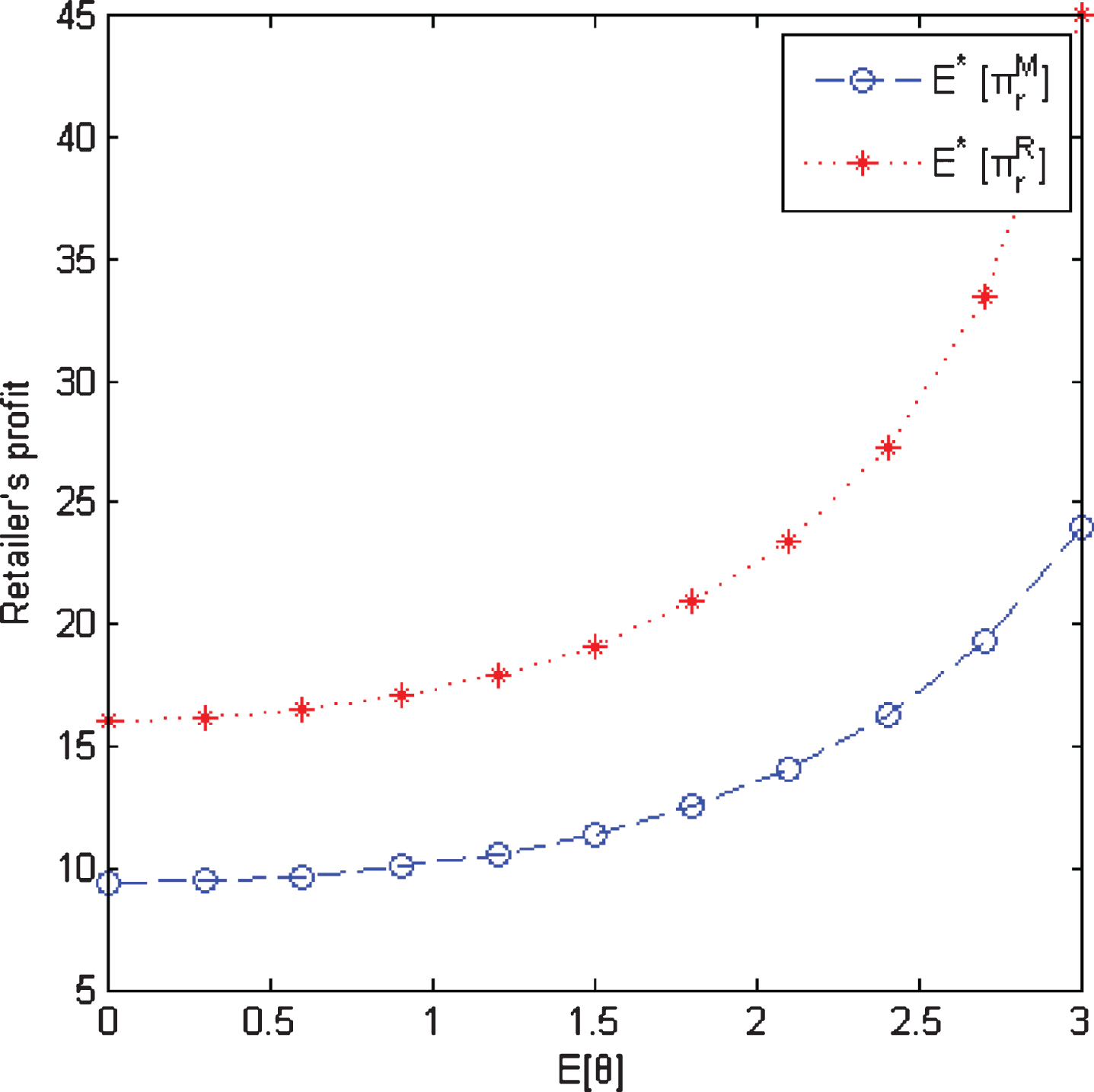
The effect of E [θ] on the expected profit of retailer.

5.3 Sensitivity of γ

In this subsection, we analyze the influence of parameter γ on the green degree, sales effort, retail price, expected profit of manufacturer, expected profit of retailer and expected channel profit in three models. The remaining parameters are assumed as follows: a = 150, c = 15, h = 1, k = 1, β = ℒ (7, 9) , θ = ℒ (1, 3).

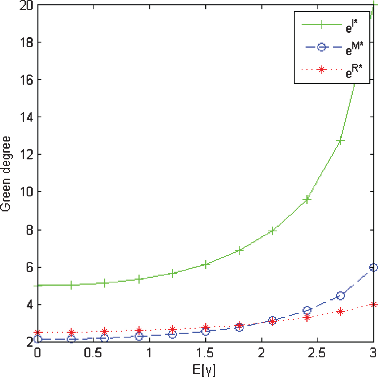
As Figure 7 shows, the green degree in these three scenarios is growing with the increase of E [γ] and is highest in integrated scenario. The green degree in manufacturer-dominant scenario is higher than that in retailer-dominant scenario when E [γ] is below a threshold in Corollary 2. While the green degree in retailer-dominant scenario is larger than that in manufacturer-dominant scenario when E [γ] is larger than this threshold. From Figure 8, we can obtain similar results that the sales effort and the expected channel profit are rising with increasing E [γ] in three scenarios and are greatest in integrated scenario.

Fig. 7

The effect of E [γ] on green degree.

Fig. 8

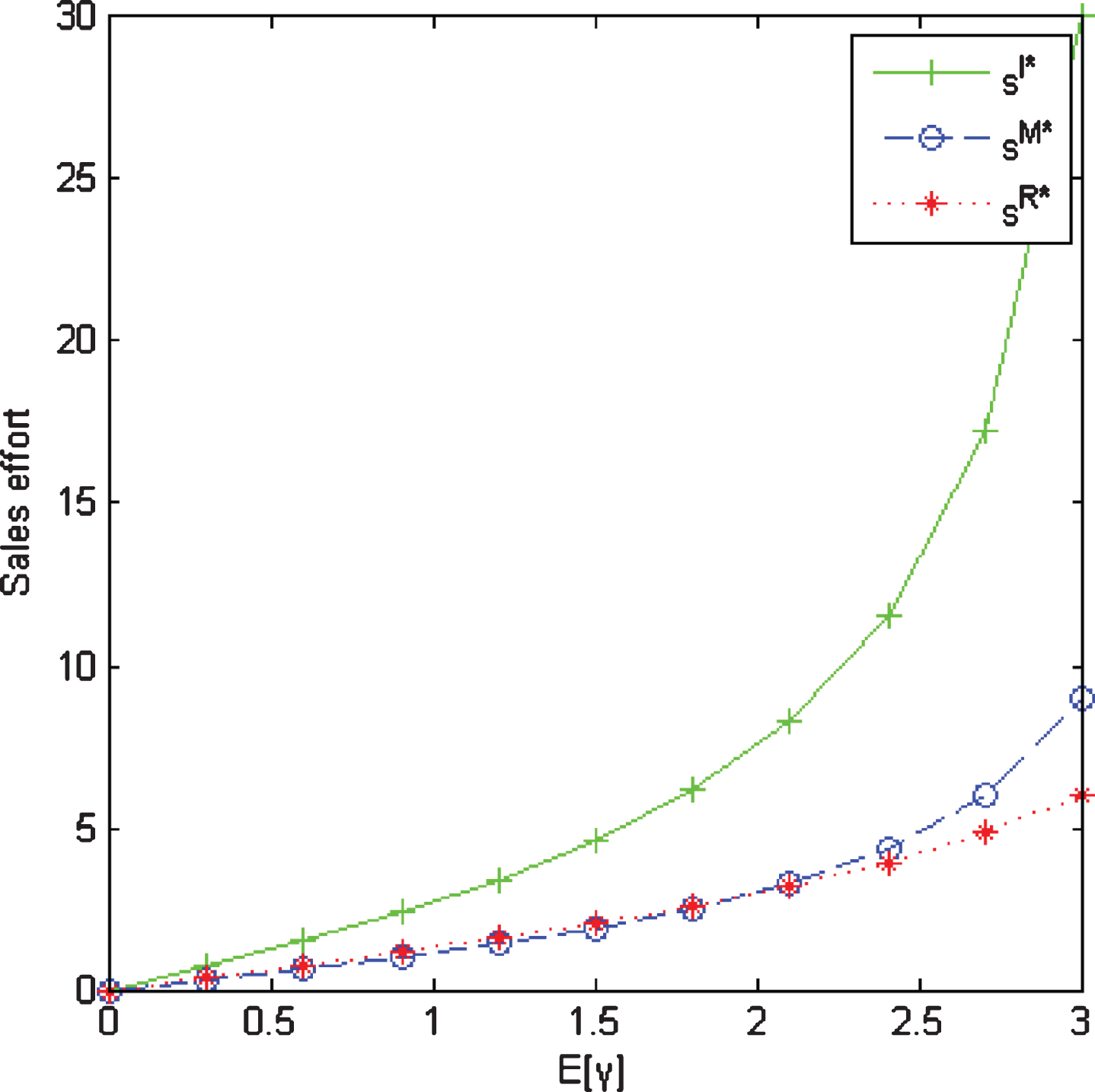
The effect of E [γ] on sales effort.

In Figure 9, we have the result that the retail price rises in these three scenarios when E [γ] increases because the sales effort investment increases with growing of E [γ]. When E [γ] is below a threshold in Corollary 3, the retail price is highest in manufacturer-dominant scenario and lowest in integrated scenario. And when E [γ] is greater than this threshold, the retail price increases quickly and is highest in retailer-dominant scenario as E [γ] increases.

Fig. 9

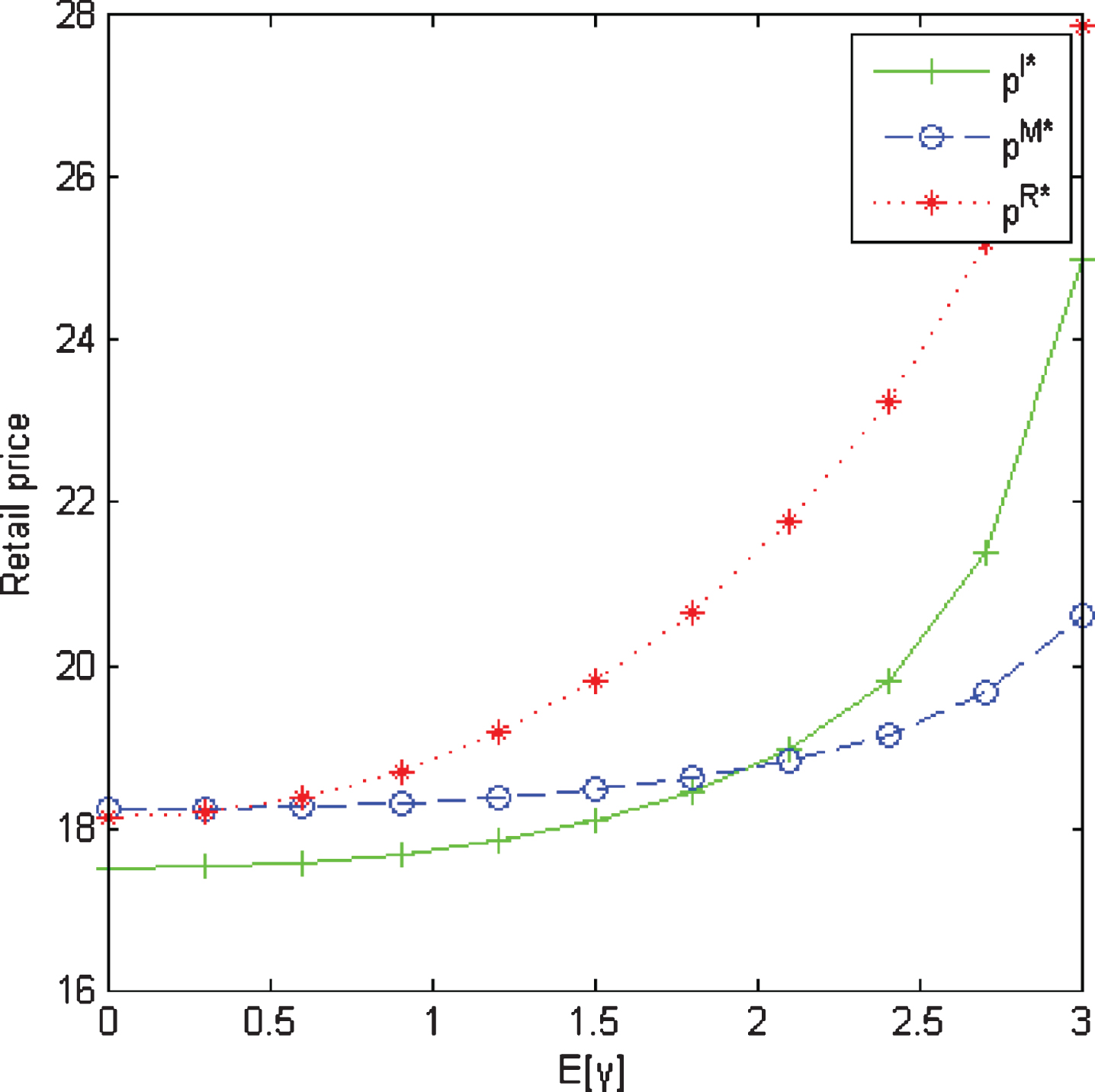
The effect of E [γ] on retail price.

Figure 10 shows that the expected channel profit is increasing in these three scenarios with rising of E [γ], and the expected channel profit is largest in integrated scenario. The results above are in line with the common sense.

Fig. 10

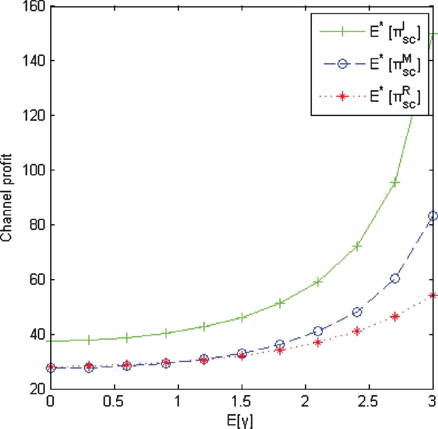
The effect of E [γ] on the expected channel profit.

As shown in Figure 11 and Figure 12, the expected profits of manufacturer and retailer increase when E [γ] rises in manufacturer-dominant scenario and retailer-dominant scenario. The increase of E [γ] leads to the expansion of demand, which results in an increase of profit. For given parameter values, the expected profit of manufacturer is higher in manufacturer-dominant scenario than that in retailer-dominant scenario. The ranking of the expected profit of retailer in such two scenarios changes as E [γ] increases.

Fig. 11

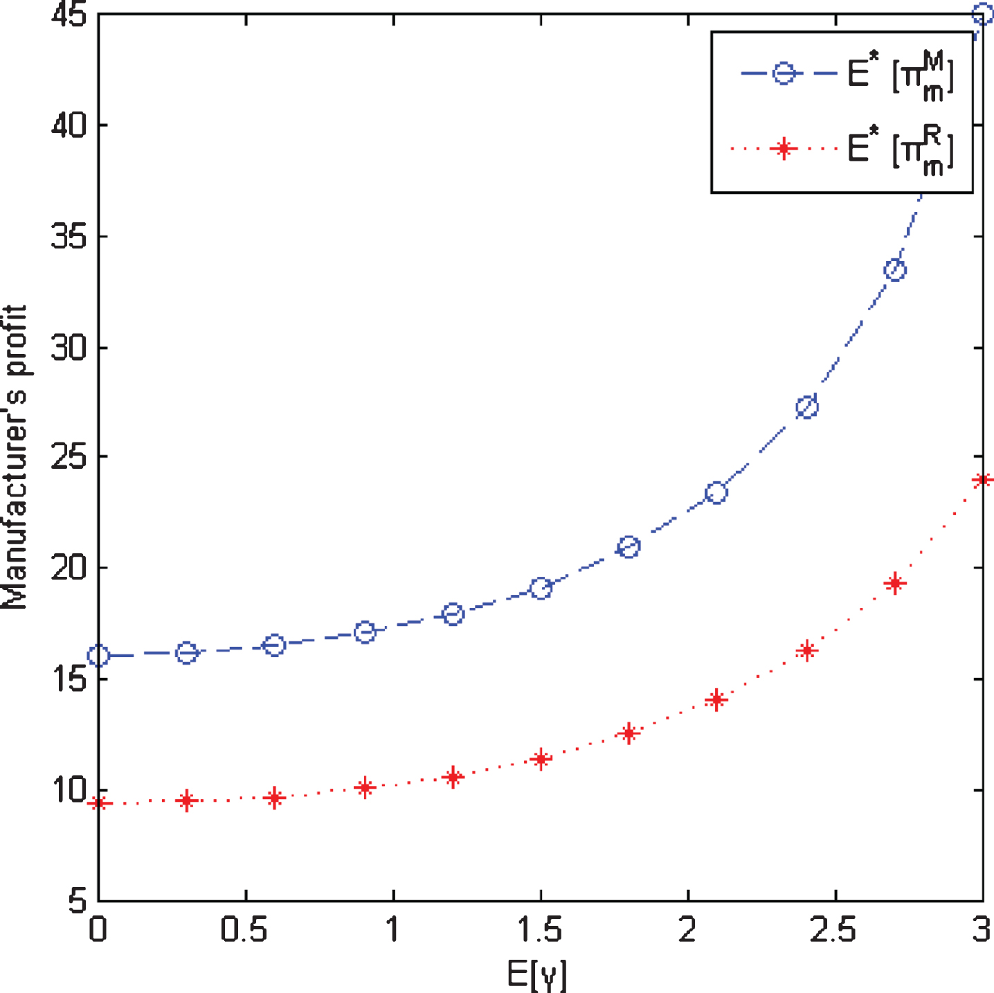
The effect of E [γ] on the expected profit of manufacturer.

Fig. 12

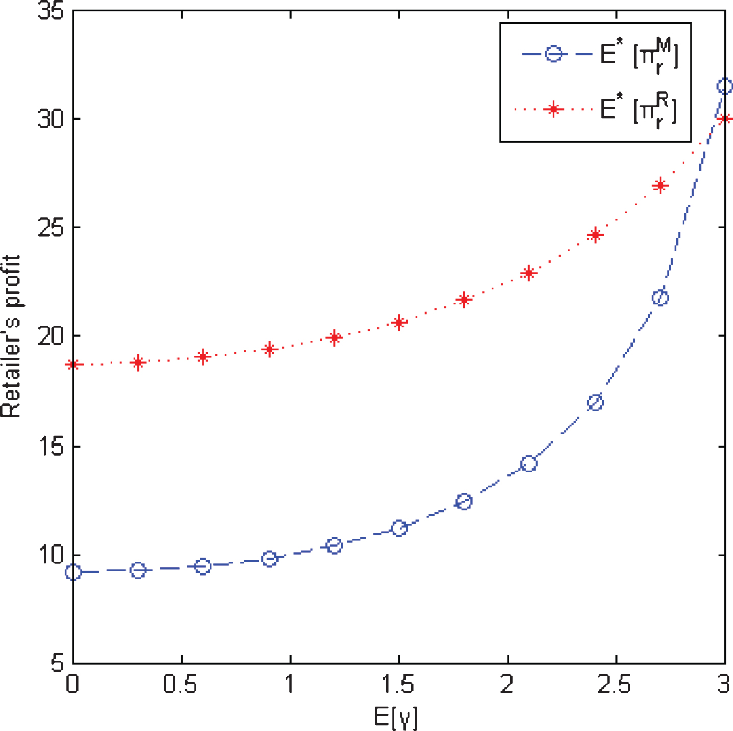
The effect of E [γ] on the expected profit of retailer.

6 Conclusion

In this paper, considering the uncertainty in the demand of new environmental-friendly products, we used uncertain variable to deal with demand due to lacking historical data. Then three models in different power structures were established to obtain the optimal green degree, pricing and sales effort decisions of green supply chain. Following that, we analyzed how power structures and uncertain parameters influence the optimal green degree, retail price and sales effort. Finally, numerical simulations are introduced to verify the correctness of the result and analyze the sensitivity of parameters.

Our study provides some managerial insights on the pricing, green degree and sales effort decisions of a two-stage supply chain under uncertain demand. Firstly, the price parameter β has a negative impact on the optimal green degree, pricing and sales effort, while the green degree parameter θ and sales effort parameter γ have positive impact on the optimal green degree, pricing and sales effort, respectively. Secondly, green degree and sales effort level are affected by the sequence of decision making, while their ranking is also related to the value of parameters. Finally, when manufacturer has high bargaining power in the supply chain, he does not necessarily benefit more from his high bargaining power. Therefore, in some cases, it is better for manufacturer to abandon the dominance.

This paper only investigated the pricing, green degree and sales effort decisions issue of green supply chain with a manufacturer and a retailer in uncertain environment. It is interesting in extending our research to the competitive of two manufacturers or retailers in the future. In addition, carbon emission reduction is encouraged all over the world, therefore the government can play an important role in green supply chain management. It will be worthy to explore the function of government strategy in pricing decision of green supply chain.

Footnotes

Appendix

Proof of Proposition 1 In the integrated scenario, by the linearity of expected value operator, the expected channel profit $E [π_{sc}^{I} (p, e, s)]$ can be expressed as:

$\begin{matrix} E [π_{sc}^{I} (p, e, s)] \\ = E [(p - c) (a - β p + θ e + γ s) - \frac{1}{2} {he}^{2} - \frac{1}{2} {ks}^{2}] \\ = \int_{0}^{1} [(p - c) (a - Φ_{1} (1 - α) p + Φ_{2} (α) e + Φ_{3} (α) s) \\ - \frac{1}{2} {he}^{2} - \frac{1}{2} {ks}^{2}] d α \\ = (p - c) (a - pE [β] + eE [θ] + sE [γ]) - \frac{1}{2} {he}^{2} - \frac{1}{2} {ks}^{2} . \end{matrix}$

After calculating, the first-order partial derivatives are as follows,

$\frac{\partial E [π_{sc}^{I} (p, e, s)]}{\partial p} = a - pE [β] + eE [θ] + sE [γ] - (p - c) E [β]$ ,

$\frac{\partial E [π_{sc}^{I} (p, e, s)]}{\partial e} = (p - c) E [γ] - ks$ ,

$\frac{\partial E [π_{sc}^{I} (p, e, s)]}{\partial s} = (p - c) E [θ] - he$ .

The second-order partial derivatives are as follows,

$\frac{\partial^{2} E [π_{sc}^{I} (p, e, s)]}{\partial p^{2}} = - 2 E [β]$ ,

$\frac{\partial^{2} E [π_{sc}^{I} (p, e, s)]}{\partial s^{2}} = - k$ ,

$\frac{\partial^{2} E [π_{sc}^{I} (p, e, s)]}{\partial e^{2}} = - h$ ,

$\frac{\partial^{2} E [π_{sc}^{I} (p, e, s)]}{\partial p \partial s} = E [γ]$ ,

$\frac{\partial^{2} E [π_{sc}^{I} (p, e, s)]}{\partial p \partial e} = E [θ]$ ,

$\frac{\partial^{2} E [π_{sc}^{I} (p, e, s)]}{\partial s \partial e} = 0$ .

By the above equations, Hessian matrix of $E [π_{sc}^{I} (p, e, s)]$ is calculated as follows, (13) $H_{1} = [\begin{matrix} - 2 E [β] & E [γ] & E [θ] \\ E [γ] & - k & 0 \\ E [θ] & 0 & - h \end{matrix}] .$

When 2kE [β] - E² [θ] >0 and 2hkE [β] - kE² [θ]) - hE² [γ] >0 holds, Hessian matrix H₁ is negative definite, and the expected channel profit $E [π_{sc}^{I} (p, e, s)]$ is jointly concave with respect to p, e and s.

Setting the first-order partial derivative as 0, we derive

$p_{sc}^{I *} = \frac{c ({kE}^{2} [θ] + {hE}^{2} [γ]) - hk (a + cE [β])}{- 2 hkE [β] + {hE}^{2} [γ] + {kE}^{2} [θ]}$ ,

$e_{sc}^{I *} = \frac{- kE [θ] (a - cE [β])}{- 2 hkE [β] + {hE}^{2} [γ] + {kE}^{2} [θ]}$ ,

$s_{sc}^{I *} = \frac{- hE [γ] (a - cE [β])}{- 2 hkE [β] + {hE}^{2} [γ] + {kE}^{2} [θ]}$ .

By substituting the above expressions into the expected channel profit E [π_sc (p, e, s)], we obtain

$E^{*} [π_{sc}^{I}] = \frac{- kh (a - cE [β])^{2}}{2 (- 2 hkE [β] + {hE}^{2} [γ] + {kE}^{2} [θ])}$ .

Then Proposition 1 is proved.

Proof of Propositions(2-3) In the manufacturer-dominant model, by the linearity of expected value operator, the expected profit of retailer $E [π_{r}^{M} (p, s)]$ can be expressed as

$\begin{matrix} E [π_{r}^{M} (p, s)] \\ = E [(p - w) (a - β p + θ e + γ s) - \frac{1}{2} {ks}^{2}] \\ = \int_{0}^{1} [(p - w) (a - Φ_{1} (1 - α) p + Φ_{2} (α) e \\ + Φ_{3} (α) s) - \frac{1}{2} {ks}^{2}] d α \\ = (p - w) (a - pE [β] + eE [θ] + sE [γ]) - \frac{1}{2} {ks}^{2} . \end{matrix}$

After calculating, the first-order partial derivatives are as follows,

$\frac{\partial E [π_{r}^{M} (p, s)]}{\partial p} = a - 2 pE [β] + eE [θ] + sE [γ] + wE [β]$ ,

$\frac{\partial E [π_{r}^{M} (p, s)]}{\partial e} = (p - w) E [γ] - ks$ .

The second-order partial derivatives are as follows,

$\frac{\partial^{2} E [π_{r}^{M} (p, s)]}{\partial p^{2}} = - 2 E [β]$ ,

$\frac{\partial^{2} E [π_{r}^{M} (p, s)]}{\partial s^{2}} = - k$ ,

$\frac{\partial^{2} E [π_{r}^{M} (p, s)]}{\partial p \partial s} = E [γ]$ .

According to the above equations, Hessian matrix of $E [π_{r}^{M} (p, s)]$ is calculated as follows: (14) $H_{2} = [\begin{matrix} - 2 E [β] & E [γ] \\ E [γ] & - k \end{matrix}] .$

When 2kE [β] - E² [γ] >0 holds, Hessian matrix H₂ is negative definite, and the expected profit of retailer $E [π_{r}^{M} (p, s)]$ is jointly concave with respect to p and s.

Setting the first-order partial derivatives as 0, we obtain (15) $p^{M} (w, e) = \frac{kwE [β] + keE [θ] + ak - {wE}^{2} [γ]}{2 kE [β] - E^{2} [γ]}$ and (16) $s^{M} (w, e) = \frac{E [γ] (a + eE [θ] - wE [β])}{2 kE [β] - E^{2} [γ]} .$

Substituting the above expressions into the expected profit of manufacturer $E [π_{m}^{M} (w, e)]$ , we have

$\begin{matrix} E [π_{m}^{M}] \\ = E [(w - c) (a - β p_{r}^{M *} (w, e) + θ e + s_{r}^{M *} (w, e) - \frac{1}{2} {he}^{2})] \\ = \frac{2 kE [β] (w - c) (a + θ - wE [β]) + e^{2} h (E^{2} [γ] - 2 kE [β])}{2 (2 kE [β] - E^{2} [γ])} . \end{matrix}$

Then, after calculating, the first-order partial derivatives of $E [π_{m}^{M} (w, e)]$ are as follows,

$\frac{\partial E [π_{m}^{M} (w, e)]}{\partial w} = \frac{- kE [β] (a + cE [β] + eE [θ] - 2 wE [β])}{2 kE [β] - E^{2} [γ]}$ ,

$\frac{\partial E [π_{m}^{M} (w, e)]}{\partial e} = \frac{eh (2 kE [β] - E^{2} [γ]) - k (w - c) E [β] E [θ]}{2 kE [β] - E^{2} [γ]}$ .

The second-order partial derivatives are as follows,

$\frac{\partial^{2} E [π_{m}^{M} (w, e)]}{\partial w^{2}} = \frac{- 2 {kE}^{2} [β]}{2 kE [β] - E^{2} [γ]}$ ,

$\frac{\partial^{2} E [π_{m}^{M} (w, e)]}{\partial e^{2}} = - h$ ,

$\frac{\partial^{2} E [π_{m}^{M} (w, e)]}{\partial w \partial e} = \frac{kE [β] E [θ]}{2 kE [β] - E^{2} [γ]}$ .

Following the above equations, Hessian matrix of $E [π_{m}^{M} (w, e)]$ is calculated as follows: (17) $H_{3} = [\begin{matrix} \frac{- 2 {kE}^{2} [β]}{2 kE [β] - E^{2} [γ]} & \frac{kE [β] E [θ]}{2 kE [β] - E^{2} [γ]} \\ \frac{kE [β] E [θ]}{2 kE [β] - E^{2} [γ]} & - h \end{matrix}] .$

When kE² [θ] +2hE² [γ] -4khE [β] <0 holds, Hessian matrix H₃ is negative definite, and the expected profit of manufacturer $E [π_{m}^{M} (w, e)]$ is jointly concave in w and e.

Setting the first-order partial derivatives as 0, we obtain

$w^{M *} = \frac{ckE [β] E^{2} [θ] - h (a + cE [β]) (2 kE [β] - E^{2} [γ])}{E [β] (- 4 hkE [β] + 2 {hE}^{2} [γ] + {kE}^{2} [θ])}$ , and $e^{M *} = \frac{- kE [θ] (a - cE [β])}{- 4 hkE [β] + 2 {hE}^{2} [γ] + {kE}^{2} [θ]}$ .

Substituting the results of w^M∗ and e^M∗ into the expressions of p^M (w, e), s^M (w, e) and the profit functions, we get

$p^{M *} = \frac{h (a + cE [β]) (E^{2} [γ] - kE [β]) + kE [β] ({cE}^{2} [θ] - 2 ah)}{E [β] (- 4 hkE [β] + 2 {hE}^{2} [γ] + {kE}^{2} [θ])}$ ,

$s^{M *} = \frac{- hE [γ] (a - cE [β])}{- 4 hkE [β] + 2 {hE}^{2} [γ] + {kE}^{2} [θ]}$ ,

$E^{*} [π_{m}^{M}] = \frac{- hk (a - cE [β])^{2}}{2 (- 4 hkE [β] + 2 {hE}^{2} [γ] + {kE}^{2} [θ])}$ ,

$E^{*} [π_{r}^{M}] = \frac{h^{2} k (a - cE [β])^{2} (2 kE [β] - E^{2} [γ])}{2 (- 4 hkE [β] + 2 {hE}^{2} [γ] + {kE}^{2} [θ])}$ ,

$E^{*} [π_{sc}^{M}] = \frac{(a - cE [β]) [{kE}^{2} [θ] - 3 h (2 kE [β] - E^{2} [γ])]}{2 (- 4 hkE [β] + 2 {hE}^{2} [γ] + {kE}^{2} [θ])}$ .

Proof of Propositions(4-5) In the retailer-dominant model, by the linearity of expected value operator, the expected profit of manufacturer $E [π_{m}^{R} (w, e)]$ can be expressed as $\begin{matrix} E [π_{m}^{R} (w, e)] \\ = E [(w - c) (a - β p + θ e + γ s) - \frac{1}{2} {he}^{2}] \\ = \int_{0}^{1} [(w - c) (a - Φ_{1} (1 - α) p + Φ_{2} (α) e \\ + Φ_{3} (α) s) - \frac{1}{2} {he}^{2}] d α \\ = (w - c) (a - pE [β] + eE [θ] + sE [γ]) - \frac{1}{2} {he}^{2} . \end{matrix}$

After calculating, the first-order partial derivatives are as follows,

$\frac{\partial E [π_{m}^{R} (w, e)]}{\partial w} = a - pE [β] + eE [θ] + sE [γ] - (w - c) E [β]$ ,

$\frac{\partial E [π_{m}^{R} (w, e)]}{\partial e} = (w - c) E [θ] - he$ .

The second-order partial derivatives are as follows

$\frac{\partial^{2} E [π_{m}^{R} (w, e)]}{\partial w^{2}} = - 2 E [β]$ ,

$\frac{\partial^{2} E [π_{m}^{R} (w, e)]}{\partial e^{2}} = - h$ .

$\frac{\partial^{2} E [π_{m}^{R} (w, e)]}{\partial w \partial e} = E [θ]$ .

According to the above equations, Hessian matrix of $E [π_{m}^{R} (w, e)]$ is (18) $H_{4} = [\begin{matrix} - 2 E [β] & E [θ] \\ E [θ] & - h \end{matrix}] .$

When 2hE [β] - E² [θ] >0, H₄ is negative definite, and the expected profit of manufacturer $E [π_{m}^{R} (w, e)]$ is jointly concave in w and e.

Setting the first-order derivatives as 0, we have

$w^{R} (p, s) = \frac{h (a - pE [β] + sE [γ] + cE [β]) - {cE}^{2} [θ]}{hE [β] - E^{2} [θ]}$ ,

$e^{R} (p, s) = \frac{E [θ] (a - pE [β] + sE [γ])}{hE [β] - E^{2} [θ]}$ .

Substituting the expressions of w^R (p, s) and e^R (p, s) into the expected profit of retailer, we have

$\begin{matrix} E [π_{r}^{R}] \\ = E [(p - w^{R} (p, s)) (a - β p + θ e^{R} (p, s) + γ s) - \frac{1}{2} {ks}^{2}] \\ = (p - w^{R} (p, s)) (a - E [β] p + E [θ] e^{R} (p, s) + E [γ] s) - \frac{1}{2} {ks}^{2} . \end{matrix}$

After calculating, the first-order partial derivatives of $E [π_{r}^{R} p, s)]$ are as follows,

$\frac{\partial E [π_{r}^{R} (p, s)]}{\partial p} = \frac{hE [β] ({chE}^{2} [β] - 4 {hpE}^{2} [β] - cE [β] E^{2} [θ] + 3 hsE [β] E [γ] + 2 pE [β] E^{2} [θ] - sE [γ] E^{2} [θ] + 3 ahE [β] - {aE}^{2} [θ])}{(hE [β] - E^{2} [θ])^{2}}$ ,

$\frac{\partial E [π_{r}^{R} (p, s)]}{\partial s} = - \frac{ch2E2[β]E[γ]-3h2E2[β]E[γ]+ksh2 E2[β]-chE[β]E2[θ]E[γ]+2h2E[β]E2[γ]+ hpE[β]E[γ]E2[θ]-2hksE[β]E2[θ]+ksE4[θ]+ 2ah2E[β]E[γ]}{(hE [β] - E^{2} [θ])^{2}},$ The second-order partial derivatives are as follows,

$\frac{\partial^{2} E [π_{r}^{R} (p, s)]}{\partial p^{2}} = \frac{- 2 {hE}^{2} [β] (2 hE [β] - E^{2} [θ])}{(hE [β] - E^{2} [θ])^{2}}$ ,

$\frac{\partial^{2} E [π_{r}^{R} (p, s)]}{\partial s^{2}} = \frac{- 2 hE [β] E^{2} [γ]}{(hE [β] - E^{2} [θ])^{2}} - k$ ,

$\frac{\partial^{2} E [π_{r}^{R} (p, s)]}{\partial p \partial s} = \frac{hE [β] E [γ] (3 hE [β] - E^{2} [θ])}{(hE [β] - E^{2} [θ])^{2}}$ . By the above equations, Hessian matrix of $E [π_{r}^{R} (p, s)]$ can be derived as follows,

(19) $H_{5} = [\begin{matrix} \frac{- 2 {hE}^{2} [β] (2 hE [β] - E^{2} [θ])}{(hE [β] - E^{2} [θ])^{2}} & \frac{hE [β] E [γ] (3 hE [β] - E^{2} [θ])}{(hE [β] - E^{2} [θ])^{2}} \\ \frac{hE [β] E [γ] (3 hE [β] - E^{2} [θ])}{(hE [β] - E^{2} [θ])^{2}} & \frac{- 2 hE [β] E^{2} [γ]}{(hE [β] - E^{2} [θ])^{2}} - k \end{matrix}] .$

When kE² [θ] +2hE² [γ] -4khE [β] <0, H₅ is negative definite. Thus, the expected profit of manufacturer $E [π_{r}^{R} (p, s)]$ is jointly concave with respect to p and s.

Setting the first-order partial derivatives as 0, we obtain

$p^{R *} = \frac{- {chkE}^{2} [β] + chE [β] E^{2} [γ] + ckE [β] E^{2} [θ] - 3 ahkE [β] + {akE}^{2} [θ]}{E [β] (- 4 hkE [β] + {hE}^{2} [γ] + 2 {kE}^{2} [θ])}$ ,

$s^{R *} = \frac{- hE [γ] (a - cE [β])}{- 4 hkE [β] + {hE}^{2} [γ] + 2 {kE}^{2} [θ]}$ ,

$w^{R *} = \frac{- 3 chkE [β]_{c} {hE}^{2} [γ] + 2 {ckE}^{2} [γ] - ahk}{- 4 hkE [β] + {hE}^{2} [γ] + 2 {kE}^{2} [θ]}$ ,

$e^{R *} = \frac{- kE [θ] (a - cE [β])}{- 4 hkE [β] + {hE}^{2} [γ] + 2 {kE}^{2} [θ]}$ ,

$E^{*} [π_{m}^{R}] = \frac{{hk}^{2} (a - cE [β])^{2} (2 hE [β] - E^{2} [θ])}{(- 4 hkE [β] + {hE}^{2} [γ] + 2 {kE}^{2} [θ])^{2}}$ ,

$E^{*} [π_{r}^{R}] = \frac{- hk (a - cE [β])^{2}}{2 (- 4 hkE [β] + {hE}^{2} [γ] + 2 {kE}^{2} [θ])}$ .

Proof of Corollary 1 Under the conditions 2kE [β] - E² [θ] >0 and 2hkE [β] - kE² [θ]) - hE² [γ] >0, we can obtain the first-order partial derivatives of the functions of retail price, green degree, sales effort, expected profit of manufacturer, expected profit of retailer and expected channel profit with respect to E [θ] and E [γ] in the optimal situation.

(1)Integrated scenario:

$\frac{\partial e^{I *}}{\partial E [θ]} = \frac{k (a - cE [β]) (2 hkE [β] - {hE}^{2} [γ] + {kE}^{2} [θ])}{(- 2 hkE [β] + {hE}^{2} [γ] + {kE}^{2} [θ])^{2}} > 0$ ,

$\frac{\partial p^{I *}}{\partial E [θ]} = \frac{2 {hk}^{2} E [θ] (a - cE [β])}{(- 2 hkE [β] + {hE}^{2} [γ] + {kE}^{2} [θ])^{2}} > 0$ ,

$\frac{\partial s^{I *}}{\partial E [θ]} = \frac{hkE [θ] E [γ] (a - cE [β])}{(- 2 hkE [β] + {hE}^{2} [γ] + {kE}^{2} [θ])^{2}} > 0$ ,

$\frac{\partial E^{*} [π_{sc}^{I}]}{\partial E [θ]} = \frac{h^{2} kE [γ] (a - cE [β])^{2}}{(2 hkE [β] - {hE}^{2} [γ] - {kE}^{2} [θ])^{2}} > 0$ ,

$\frac{\partial e^{I *}}{\partial E [γ]} = \frac{2 hkE [θ] E [γ] (a - cE [β])}{(- 2 hkE [β] + {hE}^{2} [γ] + {kE}^{2} [θ])^{2}} > 0$ ,

$\frac{\partial p^{I *}}{\partial E [γ]} = \frac{2 h^{2} kE [γ] (a - cE [β])}{(2 hkE [β] - {hE}^{2} [γ] - {kE}^{2} [θ])^{2}} > 0$ ,

$\frac{\partial s^{I *}}{\partial E [γ]} = \frac{h (a - cE [β]) (2 hkE [β] + {hE}^{2} [γ] - {kE}^{2} [θ])}{(2 hkE [β] - {hE}^{2} [γ] - {kE}^{2} [θ])^{2}} > 0$ ,

$\frac{\partial E^{*} [π_{sc}^{I}]}{\partial E [γ]} = \frac{{hk}^{2} E [θ] (a - cE [β])^{2}}{(2 hkE [β] - {hE}^{2} [γ] - {kE}^{2} [θ])^{2}} > 0$ .

$\frac{\partial D^{I *}}{\partial E [θ]} = \frac{2 h^{2} kE [β] E [γ] (a - cE [β])}{(- 2 hkE [β] + {hE}^{2} [γ] + {kE}^{2} [θ])^{2}} > 0$ ,

$\frac{\partial D^{I *}}{\partial E [γ]} = \frac{2 {hk}^{2} E [β] E [θ] (a - cE [β])}{(- 2 hkE [β] + {hE}^{2} [γ] + {kE}^{2} [θ])^{2}} > 0$ ,

(2)Manufacturer-dominant scenario:

$\frac{\partial e^{M *}}{\partial E [θ]} = \frac{k (a - cE [β]) (4 hkE [β] - 2 {hE}^{2} [γ] + {kE}^{2} [θ])}{(4 hkE [β] - 2 {hE}^{2} [γ] - {kE}^{2} [θ])^{2}} > 0$ ,

$\frac{\partial w^{M *}}{\partial E [θ]} = \frac{2 {hkE}^{2} [θ] E [γ] (a - cE [β])}{E [β] (4 hkE [β] - 2 {hE}^{2} [γ] - {kE}^{2} [θ])^{2}} > 0$ ,

$\frac{\partial p^{M *}}{\partial E [θ]} = \frac{2 hkE [θ] (a - cE [β]) (3 kE [β] - E^{2} [γ])}{E [β] (4 hkE [β] - 2 {hE}^{2} [γ] - {kE}^{2} [θ])^{2}} > 0$ ,

$\frac{\partial s^{M *}}{\partial E [θ]} = \frac{2 hkE [θ] E [γ] (a - cE [β])}{(4 hkE [β] - 2 {hE}^{2} [γ] - {kE}^{2} [θ])^{2}} > 0$ ,

$\frac{\partial E^{*} [π_{m}^{M}]}{\partial E [θ]} = \frac{{hk}^{2} E [θ] (a - cE [β])^{2}}{(4 hkE [β] - 2 {hE}^{2} [γ] - {kE}^{2} [θ])^{2}} > 0$ ,

$\frac{\partial E^{*} [π_{r}^{M}]}{\partial E [θ]} = \frac{2 h^{2} k^{2} E [θ] (a - cE [β])^{2} (- 2 kE [β] + E^{2} [γ])}{(4 hkE [β] - 2 {hE}^{2} [γ] - {kE}^{2} [θ])^{3}} > 0$ ,

$\frac{\partial E^{*} [π_{sc}^{M}]}{\partial E [θ]} = \frac{{hk}^{2} E [θ] (a - cE [β])^{2} (8 hkE [β] - 4 {hE}^{2} [γ] - {kE}^{2} [θ])}{(4 hkE [β] - 2 {hE}^{2} [γ] - {kE}^{2} [θ])^{3}} > 0$ ,

$\frac{\partial D^{M *}}{\partial E [θ]} = \frac{4 h^{2} kE [β] E [γ] (a - cE [β])}{(4 hkE [β] - 2 {hE}^{2} [γ] - {kE}^{2} [θ])^{2}} > 0$ ,

$\frac{\partial e^{M *}}{\partial E [γ]} = \frac{4 hkE [θ] E [γ] (a - cE [β])}{(4 hkE [β] - 2 {hE}^{2} [γ] - {kE}^{2} [θ])^{2}} > 0$ ,

$\frac{\partial w^{M *}}{\partial E [γ]} = \frac{2 hkE [θ] (- 2 {ckE}^{2} [β] + cE [β] E^{2} [γ] + 2 akE [β] - {aE}^{2} [γ])}{E [β] (4 hkE [β] - 2 {hE}^{2} [γ] - {kE}^{2} [θ])^{2}} > 0$ ,

$\frac{\partial p^{M *}}{\partial E [γ]} = \frac{2 hk (a - cE [β]) (2 hE [β] + E^{2} [γ])}{(4 hkE [β] - 2 {hE}^{2} [γ] - {kE}^{2} [θ])^{2}} > 0$ ,

$\frac{\partial s^{M *}}{\partial E [γ]} = \frac{(a - cE [β]) (4 hkE [β] + 2 {hE}^{2} [γ] - {kE}^{2} [θ])}{E [β] (4 hkE [β] - 2 {hE}^{2} [γ] - {kE}^{2} [θ])^{2}} > 0$ ,

$\frac{\partial E^{*} [π_{m}^{M}]}{\partial E [γ]} = \frac{2 h^{2} kE [γ] (a - cE [β])^{2}}{(4 hkE [β] - 2 {hE}^{2} [γ] - {kE}^{2} [θ])^{2}} > 0$ ,

$\frac{\partial E^{*} [π_{r}^{M}]}{\partial E [γ]} = \frac{h^{2} kE [θ] (a - cE [β])^{2} (4 hkE [β] - 2 {hE}^{2} [γ] + {kE}^{2} [θ])}{(4 hkE [β] - 2 {hE}^{2} [γ] - {kE}^{2} [θ])^{3}} > 0$ ,

$\frac{\partial E^{*} [π_{sc}^{M}]}{\partial E [γ]} = \frac{h^{2} kE [θ] (a - cE [β])^{2} (12 hkE [β] - 6 {hE}^{2} [γ] - {kE}^{2} [θ])^{2}}{(4 hkE [β] - 2 {hE}^{2} [γ] - {kE}^{2} [θ])^{3}} > 0$ .

$\frac{\partial D^{M *}}{\partial E [γ]} = \frac{2 {hk}^{2} E [β] E [θ] (a - cE [β])}{(4 hkE [β] - 2 {hE}^{2} [γ] - {kE}^{2} [θ])^{2}} > 0$ ,

(3)Retailer-dominant scenario:

$\frac{\partial e^{R *}}{\partial E [θ]} = \frac{k (a - cE [β]) (4 hkE [β] - {hE}^{2} [γ] + 2 {kE}^{2} [θ])}{(4 hkE [β] - {hE}^{2} [γ] - 2 {kE}^{2} [θ])^{2}} > 0$ ,

$\frac{\partial w^{R *}}{\partial E [θ]} = \frac{4 {hk}^{2} E [θ] (a - cE [β]) (4 hkE [β] - {hE}^{2} [γ] + 2 {kE}^{2} [θ])}{(4 hkE [β] - {hE}^{2} [γ] - 2 {kE}^{2} [θ])^{2}} > 0$ ,

$\frac{\partial p^{R *}}{\partial E [θ]} = \frac{2 hkE [θ] (2 akE [β] + {aE}^{2} [γ] - 2 {ckE}^{2} [β] - cE [β] E^{2} [γ])}{E [β] (4 hkE [β] - {hE}^{2} [γ] - 2 {kE}^{2} [θ])^{2}} > 0$ ,

$\frac{\partial s^{R *}}{\partial E [θ]} = \frac{4 hkE [θ] E [γ] (a - cE [β])}{(4 hkE [β] - {hE}^{2} [γ] - 2 {kE}^{2} [θ])^{2}} > 0$ ,

$\frac{\partial E^{*} [π_{m}^{R}]}{\partial E [θ]} = \frac{{hk}^{2} E [θ] (a - cE [β])^{2} (4 hkE [β] + {hE}^{2} [γ] - 2 {kE}^{2} [θ])}{(4 hkE [β] - {hE}^{2} [γ] - 2 {kE}^{2} [θ])^{3}} > 0$ ,

$\frac{\partial E^{*} [π_{r}^{R}]}{\partial E [θ]} = \frac{2 {hk}^{2} E [θ] (a - cE [β])^{2}}{(4 hkE [β] - {hE}^{2} [γ] - 2 {kE}^{2} [θ])^{2}} > 0$ ,

$\frac{\partial E^{*} [π_{sc}^{R}]}{\partial E [θ]} > 0$ ,

$\frac{\partial e^{R *}}{\partial E [γ]} = \frac{2 hkE [θ] E [γ] (a - cE [β])}{(4 hkE [β] - {hE}^{2} [γ] - 2 {kE}^{2} [θ])^{2}} > 0$ ,

$\frac{\partial w^{R *}}{\partial E [γ]} = \frac{2 h^{2} kE [γ] (a - cE [β])}{(4 hkE [β] - {hE}^{2} [γ] - 2 {kE}^{2} [θ])^{2}} > 0$ ,

$\frac{\partial p^{R *}}{\partial E [γ]}$

$= \frac{2 hkE [γ] (a - cE [β]) (- 3 {chE}^{2} [β] + cE [β] E^{2} [θ] + 3 ahE [β] - {aE}^{2} [θ])}{E [β] (4 hkE [β] - {hE}^{2} [γ] - 2 {kE}^{2} [θ])^{2}} > 0$ ,

$\frac{\partial s^{R *}}{\partial E [γ]} = \frac{h (a - cE [β]) (4 hkE [β] + {hE}^{2} [γ] - 2 {kE}^{2} [θ])}{(4 hkE [β] - {hE}^{2} [γ] - 2 {kE}^{2} [θ])^{2}} > 0$ ,

$\frac{\partial E^{*} [π_{m}^{R}]}{\partial E [γ]} = \frac{- 2 h^{2} k^{2} E [γ] (a - cE [β])^{2} (2 hE [β] - E^{2} [θ])}{(4 hkE [β] - {hE}^{2} [γ] - 2 {kE}^{2} [θ])^{3}} > 0$ ,

$\frac{\partial E^{*} [π_{r}^{R}]}{\partial E [γ]} = \frac{h^{2} kE [γ] (a - cE [β])^{2}}{(4 hkE [β] - {hE}^{2} [γ] - 2 {kE}^{2} [θ])^{2}} > 0$ ,

$\frac{\partial E^{*} [π_{sc}^{R}]}{\partial E [γ]} > 0$ .

$\frac{\partial D^{R *}}{\partial E [θ]} = \frac{4 h^{2} kE [β] E [γ] (a - cE [β])}{E [β] (4 hkE [β] - {hE}^{2} [γ] - 2 {kE}^{2} [θ])^{2}} > 0$ ,

$\frac{\partial D^{R *}}{\partial E [γ]} = \frac{4 {hk}^{2} E [β] E [θ] (a - cE [β])}{E [β] (4 hkE [β] - {hE}^{2} [γ] - 2 {kE}^{2} [θ])^{2}} > 0$ .

Proof of Corollary 2

e^I∗ - e^M∗

$= \frac{kE [θ] (a - cE [β]) (2 kE [β] - E^{2} [γ])}{(2 hkE [β] - {hE}^{2} [γ] - {kE}^{2} [θ]) (4 hkE [β] - 2 {hE}^{2} [γ] - {kE}^{2} [θ])} > 0$ ,

e^I∗ - e^R∗

$= \frac{k^{2} E [θ] (a - cE [β]) (2 hE [β] - E^{2} [θ])}{(2 hkE [β] - {hE}^{2} [γ] - {kE}^{2} [θ]) (4 hkE [β] - {hE}^{2} [γ] - 2 {kE}^{2} [θ])} > 0$ ,

e^M∗ - e^R∗

$= \frac{kE [θ] (a - cE [β]) ({hE}^{2} [γ] - {kE}^{2} [θ])}{(4 hkE [β] - {hE}^{2} [γ] - 2 {kE}^{2} [θ]) (4 hkE [β] - 2 {hE}^{2} [γ] - {kE}^{2} [θ])}$ .

s^I∗ - s^M∗

$= \frac{h^{2} E [γ] (a - cE [β]) (2 kE [β] - E^{2} [γ])}{(2 hkE [β] - {hE}^{2} [γ] - {kE}^{2} [θ]) (4 hkE [β] - 2 {hE}^{2} [γ] - {kE}^{2} [θ])} > 0$

s^I∗ - s^R∗

$= \frac{hkE [γ] (a - cE [β]) (2 hE [β] - E^{2} [θ])}{(2 hkE [β] - {hE}^{2} [γ] - {kE}^{2} [θ]) (4 hkE [β] - {hE}^{2} [γ] - 2 {kE}^{2} [θ])} > 0$ ,

s^M∗ - s^R∗

$= \frac{hE [γ] (a - cE [β]) ({hE}^{2} [γ] - {kE}^{2} [θ])}{(4 hkE [β] - {hE}^{2} [γ] - 2 {kE}^{2} [θ]) (4 hkE [β] - 2 {hE}^{2} [γ] - {kE}^{2} [θ])}$ .

$E^{*} [π_{sc}^{I}] - E^{*} [π_{sc}^{M}] = \frac{h^{2} (4 k^{2} E [β] - 4 kE [β] E^{2} [γ] + E^{4} [γ])}{(2 hkE [β] - {hE}^{2} [γ] - {kE}^{2} [θ]) (4 hkE [β] - 2 {hE}^{2} [γ] - {kE}^{2} [θ])}$ ,

$E^{*} [π_{sc}^{I}] - E^{*} [π_{sc}^{R}] = \frac{k^{2} (4 h^{2} E [β] - 4 hE [β] E^{2} [θ] + E^{4} [θ])}{(2 hkE [β] - {hE}^{2} [γ] - {kE}^{2} [θ]) (4 hkE [β] - {hE}^{2} [γ] - 2 {kE}^{2} [θ])}$

$E^{*} [π_{sc}^{M}] - E^{*} [π_{sc}^{R}] = \frac{hk ({hE}^{2} [γ] - {kE}^{2} [θ]) (16 {hkE}^{2} [β] - 10 E [β] ({hE}^{2} [γ] + {kE}^{2} [θ]) + 3 E^{2} [γ] E^{2} [θ]) + h^{3} E^{6} [γ] - k^{3} E^{6} [θ]}{(4 hkE [β] - {hE}^{2} [γ] - 2 {kE}^{2} [θ]) (4 hkE [β] - 2 {hE}^{2} [γ] - {kE}^{2} [θ])}$ .

When hE² [γ] = kE² [θ], we have e^M∗ = e^R∗, s^M∗ = s^R∗ and $E^{*} [π_{sc}^{M}] = E^{*} [π_{sc}^{R}]$ .

When hE² [γ] > kE² [θ], we have e^M∗ > e^R∗, s^M∗ > s^R∗ and $E^{*} [π_{sc}^{M}] > E^{*} [π_{sc}^{R}]$ .

When hE² [γ] < kE² [θ], we have e^M∗ < e^R∗, s^M∗ < s^R∗ and $E^{*} [π_{sc}^{M}] < E^{*} [π_{sc}^{R}]$ .

Proof of Corollary 3

$p^{I *} - p^{M *} = \frac{h(2chk2E3[β]-kE2[β](3chE2[γ]+2ckE2[θ]+2ahk)+cE2[γ]E[β](hE2[γ]-kE2[θ]) -akE[β])(3hE2[γ]-2kE2[θ])-aE2[γ](hE2[γ]+kE2[θ])}{E [β] (2 hkE [β] - {hE}^{2} [γ] - {kE}^{2} [θ]) (4 hkE [β] - 2 {hE}^{2} [γ] - {kE}^{2} [θ])}$

$p^{I *} - p^{R *} = \frac{k(2chk2E3[β]-hE2[β](3ckE2[θ]+2chE2[γ]+2ahk)+cE2[θ]E[β](kE2[θ]-hE2[γ])-ahE[β])(3kE2[θ]-2hE2[γ])-aE2[θ](kE2[θ]+hE2[γ]))}{E [β] (2 hkE [β] - {hE}^{2} [γ] - {kE}^{2} [θ]) (4 hkE [β] - {hE}^{2} [γ] - 2 {kE}^{2} [θ])}$

$p^{M *} - p^{R *} = \frac{({hE}^{2} [γ] - {kE}^{2} [θ]) ({chkE}^{2} [β] - (ahk + {chE}^{2} [γ] + {ckE}^{2} [θ]) E [β] + {ahE}^{2} [γ] + {akE}^{2} [θ])}{E [β] (4 hkE [β] - {hE}^{2} [γ] - 2 {kE}^{2} [θ]) (4 hkE [β] - 2 {hE}^{2} [γ] - {kE}^{2} [θ])}$

When hE² [γ] = kE² [θ], we have p^M∗ = p^R∗.

When $\frac{E^{2} [γ]}{k} < E [β] < \frac{2 E^{2} [γ]}{k}$ , p^I∗ is the biggest.

When hE² [γ] > kE² [θ], we have p^M∗ > p^R∗.

When $\frac{2 E^{2} [γ]}{k} < E [β] < \frac{a}{c}$ , p^I∗ is the lowest.

Proof of Corollary 4

$E^{*} [π_{m}^{M}] - E^{*} [π_{m}^{R}] = \frac{hk (a - cE [β])^{2} (8 h^{2} k^{2} E^{2} [β] - 2 hkE [β] (2 {hE}^{2} [γ] + 5 {kE}^{2} [θ]) + h^{2} E^{4} [γ] + 3 k^{2} E^{4} [θ] + 2 {hkE}^{2} [γ] E^{2} [θ])}{2 (4 hkE [β] - {hE}^{2} [γ] - 2 {kE}^{2} [θ]) (4 hkE [β] - 2 {hE}^{2} [γ] - {kE}^{2} [θ])}$

When hE² [γ] > kE² [θ], we have $E^{*} [π_{m}^{M}] > E^{*} [π_{m}^{R}]$ .

When hE² [γ] = kE² [θ], we have $E^{*} [π_{m}^{M}] = E^{*} [π_{m}^{R}]$ .

When hE² [γ] < kE² [θ] and $\frac{E^{2} [γ]}{2 k} + \frac{E^{2} [θ]}{2 h} < E [β] < \frac{2 {hE}^{2} [γ] + 5 {kE}^{2} [θ] + \sqrt{k^{2} E^{4} [θ] - 4 h^{2} E^{4} [γ] + 4 {hkE}^{2} [θ] E^{2} [γ]}}{8 hk}$ , we have $E^{*} [π_{m}^{R}] > E^{*} [π_{m}^{M}]$ .

When hE² [γ] < kE² [θ] and $\frac{2 {hE}^{2} [γ] + 5 {kE}^{2} [θ] + \sqrt{k^{2} E^{4} [θ] - 4 h^{2} E^{4} [γ] + 4 {hkE}^{2} [θ] E^{2} [γ]}}{8 hk} < E [β] < \frac{a}{c}$ , we have $E^{*} [π_{m}^{M}] > E^{*} [π_{m}^{R}]$ .

Proof of Corollary 5

$E^{*} [π_{r}^{M}] - E^{*} [π_{r}^{R}] = \frac{hk (a - cE [β])^{2} (8 h^{2} k^{2} E^{2} [β] - 2 hkE [β] (5 {hE}^{2} [γ] + 2 {kE}^{2} [θ]) + 3 h^{2} E^{4} [γ] + k^{2} E^{4} [θ] + 2 {hkE}^{2} [γ] E^{2} [θ])}{(4 hkE [β] - {hE}^{2} [γ] - 2 {kE}^{2} [θ]) (4 hkE [β] - 2 {hE}^{2} [γ] - {kE}^{2} [θ])}$

When hE² [γ] > kE² [θ] and $\frac{E^{2} [γ]}{2 k} + \frac{E^{2} [θ]}{2 h} < E [β] < \frac{5 {hE}^{2} [γ] + 2 {kE}^{2} [θ] + \sqrt{h^{2} E^{4} [γ] - 4 k^{2} E^{4} [θ] + 4 {hkE}^{2} [θ] E^{2} [γ]}}{8 hk}$ , we have $E^{*} [π_{r}^{M}] > E^{*} [π_{r}^{R}]$ .

When hE² [γ] > kE² [θ] and $\frac{5 {hE}^{2} [γ] + 2 {kE}^{2} [θ] + \sqrt{h^{2} E^{4} [γ] - 4 k^{2} E^{4} [θ] + 4 {hkE}^{2} [θ] E^{2} [γ]}}{8 hk} < E [β] < \frac{a}{c}$ , we have $E^{*} [π_{r}^{R}] > E^{*} [π_{r}^{M}]$ .

When hE² [γ] = kE² [θ], we have $E^{*} [π_{r}^{M}] = E^{*} [π_{r}^{R}]$ .

When hE² [γ] < kE² [θ], we have $E^{*} [π_{r}^{R}] > E^{*} [π_{r}^{M}]$ .

References

Basiri

and Heydari

, A mathematical model for green supply chain coordination with sub-stitutable products, Journal of Cleaner Production 145 (2017), 232–249.

Cao

G.Z.

, Qin

and Cheng

J.M.

, Study on the evaluation system of the enterprise’s “green degree”, East China Economic Management 20(9) (2006), 18–20.

Chen

, Peng

, Liu

Z.B.

and Zhao

R.Q.

, Pricing and effort decisions for a supply chain with uncertain information, International Journal of Production Research 55(1) (2017), 1–21.

Cherian

and Jacob

, Green marketing: a study of consumers attitude towards environment friendly products, International Journal of Asian Social Science 8(12) (2012), 117–126.

Ertek

and Griffn

P.M.

, Supplier-and buyer-driven channels in a two-stage supply chain, IIE Transactions 34(8) (2002), 691–700.

Ghosh

and Shah

, Supply chain analysis under green sensitive consumer demand and cost sharing contract, International Journal of Production Economics 164 (2015), 319–329.

Giri

B.C.

, Bardhan

and Maiti

, Coordinating a three-layer supply chain with uncertain demand and random yield, International Journal of Production Research 54(8) (2016), 2499–2518.

Haytko

D.L.

and Matulich

, Green advertising and environmentally responsible consumer behaviors: Linkages examined, Journal of Management and Marketing Research 1 (2008), 2–11.

https://www.gfk.com/fileadmin/user_upload/downloads/Global_Studies/Global-GfK-survey_Environmental-values-ethical-shopping_2015.pdf

10.

https://www.unenvironment.org/news-and-stories/press-release/human-health-dire-straits-if-urgent-actions-are-not-made-protect

11.

Hua

Z.S.

and Li

S.J.

, Impacts of demand uncertainty on retailers dominance and manufacturer-retailer supply chain cooperation, Omega 36(5) (2008), 697–714.

12.

Huang

and Ke

, Pricing decision problem for substitutable products based on uncertainty theory, Journal of Intelligent Manufacturing 28(3) (2017), 503–514.

13.

Joshi

and Rahman

, Factors affecting green purchase behaviour and future research directions, International Strategic Management Review 128(3) (2015), 128–143.

14.

Kahneman

and Tversky

, Prospect theory: an analysis of decisions under risk, Econometrica 47(2) (1979), 263–291.

15.

, Huang

and Gao

X.Y.

, Pricing decision problem in dual-channel supply chain based on experts’ belief degrees, Soft Computing 22(17) (2018), 5683–5698.

16.

, Zhu

M.Y.

, Jiang

Y.S.

and Li

Z.H.

, Pricing policies of a competitive dual-channel green supply chain, Journal of Cleaner Production 112 (2016), 2029–2042.

17.

Liu

, Uncertainty Theory, 2nd ed., Springer-Verlag, Berlin, 2007.

18.

Liu

, Uncertainty theory: a branch of mathematics for modeling human uncertainty, Springer-Verlag, Berlin, 2010.

19.

Liu

, Why is there a need for uncertainty theory? Journal of Uncertain Systems 6(1) (2012), 3–10.

20.

Liu

Z.G.

, Anderson

T.D.

and Cruz

J.M.

, Consumer environmental awareness and competition in two-stage supply chains, European Journal of Operational Research 218(3) (2012), 602–613.

21.

, Wang

H.Y.

and Shang

, Supply chain channel strategies with quality and marketing effort-dependent demand, International Journal of Production Economics 144(2) (2013), 572–581.

22.

McGuire

T.W.

and Staelin

, An industry equilibrium analysis of downstream vertical integration, Marketing Science 2(2) (1983), 161–191.

23.

Mills

E.S.

, Uncertainty and price theory, Quarterly Journal of Economics 73(1) (1959), 116–139.

24.

Pan

, Lai

K.K.

, Leung

S.C.H.

and Xiao

, Revenue-sharing versus wholesale price mechanisms under different channel power structures, European Journal of Operational Research 203(2) (2010), 532–538.

25.

Sang

S.J.

, Pricing and level decisions with a risk averse retailer in an uncertain green supply chain, International of Applied Mathematics 48(3) (2018), 14–20.

26.

Shen

J.Y.

and Zhu

, Uncertain supply chain problem with price and effort, International Journal of Fuzzy Systems 20(4) (2018), 1145–1158.

27.

Shi

R.X.

, Zhang

and Ru

, Impacts of power structure on supply chains with uncertain demand, Production and Operations Management Society 22(5) (2013), 1–18.

28.

Syaekhoni

M.A.

, Alfian

and Kwon

Y.S.

, Customer purchasing behavior analysis as alternatives for supporting in-store green marketing decision-making, Sustainability 9(11) (2017), 1–22.

29.

Z.H.

and Pagell

, Balancing priorities: decision-making in sustainable supply chain management, Journal of Operations Management 29(6) (2011), 577–590.

30.

Z.W.

, Peng

Z.X.

, Yang

and Chen

X.D.

, An improved shapley value method for a green supply chain income distribution mechanism, International Journal of Environment Research and Public Health 15(9) (2018), 1976.

31.

Yang

D.Y.

and Xiao

T.J.

, Pricing and level decisions of a green supply chain with governmental interventions under fuzzy uncertainties, Journal of Cleaner Production 149 (2017), 1174–1187.

32.

Zhao

and Wei

, The coordinating contracts for a fuzzy supply chain with effort and price dependent demand, Applied Mathematical Modelling 38 (2014), 2476–2489.

33.

Zhao

, Xia

X.H.

and Yu

G.D.

, Buyback contract of reverse supply chains with different risk attitudes under fuzzy demands, Journal of Intelligent and Fuzzy Systems 34(1) (2018), 47–56.