A similarity measure determines the similarity between two objects. As important roles of similarity measure in chance theory, this paper introduces the concept of partial similarity measure for two uncertain random variables. Based on maximum similarity principle, partial similarity measure are used to recognize pattern problems. As an application in finance, partial similarity measure is applied to optimize portfolio selection of uncertain random returns via Monte-Carlo simulation and craw search algorithm.
A similarity measure characterizes the similarity between two objects and can be formulated as inverse of distance measure. In general, the similarity measures can be considered as the suitable decreasing functions of distance measures. In order to characterize similarity measure of two indeterminate phenomena, Zwich et al. [31] proposed several similarity measures of fuzzy sets and compared them in numerical examples. As an application of similarity measure in pattern recognition, Li and Cheng [17] presented the concept of similarity measure for intuitionistic fuzzy sets. After that Li et al. [16] established some similarity measures between two fuzzy variables via credibility measure. Also, it is mentioned several authors devoted their works to the topic of similarity measure, for instance [7, 28].
As another type of modeling indeterminacy, Liu [20] presented uncertainty theory as a branch of mathematics. After that, Liu [20] presented the important concepts of uncertain variable and uncertainty distribution. Then, a sufficient and necessary condition for a function being an uncertainty distribution was established by Peng and Iwamura [26]. Moreover, In order to rank uncertain variables, Liu [22] proposed the concept of expected value. In order to measure similarity between two uncertain variables, Li and liu [19] proposed several similarity measures and applied them to pattern recognition.
In order to model phenomena including randomness and uncertainty simultaneously, Liu [23] presented the concept of uncertain random variables, chance distributions, expected values and variances. Following that, Liu [24] proved the operational law of uncertain random variable and the formula of expected value. Ahmadzade et al. [5] studied variance of an uncertain random variable through inverse uncertainty distribution. In order to measure the indeterminacy of an uncertain random variable, Ahmadzade et al. [3, 4] proposed the concepts of partial and quadratic partial entropies for uncertain random variables, respectively. After that, Ahmadzade and Gao [1] introduced the concept of covariance for two uncertain random variables and obtained a formula for calculating it via inverse uncertainty distributions. They proved that the variance of sum of uncertain random variables can be written as a linear function of variance and covariance function of uncertain random variables. By invoking this major, they optimize the portfolio selection problem of uncertain random returns via mean-variance-covariance model easily with Lingo software. But, in many real-world optimization problems, the objective function may be very complex and may have a large number of local optima.
In such cases, classical optimization methods are usually failed and may be trapped at local optima. Hence, due to the significant performance that new metaheuristic algorithms have shown in solving such problems, these algorithms are considered by many researchers. Some of the well-known new metaheuristic algorithms are as follows: Genetic Algorithms (GA) [13], Particle Swarm Optimization (PSO) [15], cuckoo search algorithm [29], Firefly Algorithm (FA) [30], etc. Recently, Based on the intelligent behavior of crows, a new metaheuristic algorithm called Crow Search Algorithm (CSA) [6] has been introduced for solving constrained optimization problems. CSA is a population-based optimization algorithm, and includes only two adjustable parameters (flight length and awareness probability) that makes it very attractive for various applications. Therefore, in this paper, we propose the concept of partial similarity measure and applied to portfolio selection model of uncertain random returns. Since the similarity-mean-variance model is very complex in optimization. The CSA algorithm is used to solve the similarity-mean-variance portfolio selection model.
The rest of this paper is organized as follows. In Section 2, some basic concepts in uncertainty theory and chance theory are reviewed. In Section 3, a definition of partial similarity measure of two uncertain random variables is presented and several examples are derived. Based on maximum similarity principle, we apply the partial similarity measure to the case of pattern recognition, in Section 4. Based on similarity-mean-variance model, we optimize the portfolio selection problem by Monte-Carlo simulation and craw search algorithm, in Section 5. Finally, some conclusions are provided in Section 6.
Preliminaries
In this section, we review some concepts of uncertain variables and uncertain random variables. And some relative properties are also reviewed.
Uncertain variables
In this subsection, we provide several definitions and elementary concepts of uncertainty theory that will be used in the next sections. For more details, the reader refers to [20, 21].
Let ℒ be a σ-algebra on a nonempty set Γ. A set function ℳ: ℒ → [0, 1] is called an uncertain measure if it satisfies three axioms (i), (ii), (iii):
(i) (Normality) ℳ{Γ} =1 for the universal set Γ.
(ii) (Duality) ℳ{Λ} + ℳ{Λc} =1 for any event Λ.
(iii) (Subadditivity) For every countable sequence of events Λ1, Λ2, ⋯ , we have
Then the triple (Γ, ℒ, ℳ) is called uncertainty space. Next, the product uncertain measure was proposed by Liu [21] via the following axiom.
(iv) (Product Axiom) Let (Γk, ℒk, ℳk) be uncertainty spaces for k = 1, 2, ⋯ the product uncertain measure ℳ is an uncertain measure satisfying
where Λk are arbitrarily chosen events from ℒk for k = 1, 2, ⋯ , respectively.
Definition 1. An uncertain variable ξ is a function from an uncertainty space (Γ, ℒ, ℳ) to the set of real numbers such that {ξ ∈ B} is an event for any Borel set B.
Definition 2. The uncertain variables ξ1, ξ2, ⋯ , ξn are said to be independent if
for any Borel sets B1, B2, ⋯ , Bn.
Theorem 1.Let ξ1, ξ2, ⋯ , ξn be independent uncertain variables, and f1, f2, ⋯ , fn be measurable functions. Then f1 (ξ1) , f2 (ξ2) , ⋯ , fn (ξn) are independent uncertain variables.
Definition 3. (Liu [21]) Let ξ be an uncertain random variable. Then its chance distribution is defined as
for any x ∈ ℛ .
Definition 4.(Liu [21]) Let ξ be an uncertain variable with regular uncertainty distribution Φ (x). Then the inverse function Φ-1 (x) is called the inverse uncertainty distribution of ξ.
Theorem 2.(Liu [21]) Let ξ1, ⋯ , ξn be independent uncertain variables with regular uncertainty distributions Φ1, Φ2, ⋯ , Φn, respectively. If f (x1, ⋯ , xn) is strictly increasing with respect to x1, ⋯ , xm and decreasing with respect to xm+1, ⋯ , xn thenξ = f (ξ1, ξ2, ⋯ , ξn) is an uncertain variable with inverse uncertainty distribution
For characterize difference between two uncertain variables, Li and Liu [19] presented the concept of distance for two uncertain variables.
Definition 5. (Li and Liu [19]) Let τ1 and τ2 be two uncertain variable with uncertainty distributions Φ1 and Φ2, respectively. The distance of τ1 and τ2 is defined by
Since inverse uncertainty distributions play important roles in uncertainty theory, Gao et al. [11] presented the distance of two uncertain variables based on their inverse uncertainty distributions in the following theorem.
Theorem 3.(Gao et al. [12]) Let τ1 and τ22 be two uncertain variable with uncertainty distributions Φ1 and Φ2, respectively. The distance of τ1 and τ2 is
In order to characterize the similarity of two uncertain variables via uncertainty distributions, Li and Liu [18] introduced the concept of similarity measure of two uncertain variables.
Definition 6. (Li and Liu [19]) Let X be a set of uncertain variables on the uncertainty space (Γ, ℒ, ℳ). A real valued function s (τ1, τ2) on the Cartesian product X × X is a similarity measure if, for any τ1, τ2 ; τ3 ∈ X, it satisfies the following conditions:
i) 0 ≤ s (τ1, τ2) ≤1,
ii) s (τ1, τ2) =1 iff τ1 = τ2,
iii) s (τ1, τ2) = s (τ2, τ1) ,
iv) , then s (τ2, τ3) ≤ s (τ1, τ3) and s (τ1, τ2) ≤ s (τ1, τ3).
It is clear that we can calculate a similarity of two uncertain variables via their distance. Thus, we can express the relationship between similarity and distance by invoking several functions as follows:
which, they are all strictly decreasing functions such that 0 ≤ gi (t) ≤1, i = 1, 2, 3, ∀ t ≥ 0 . We can call gi’s generator functions.
Uncertain random variable
The chance space is refer to the product (Γ, ℒ, ℳ) × (Ω, , Pr), in which (Γ, ℒ, ℳ) is an uncertainty space and (Ω, , Pr) is a probability space, respectively.
Definition 7. (Liu [23]) Let (Γ, ℒ, ℳ) × (Ω, , Pr) be a chance space, and Θ ∈ ℒ × be an uncertain random event. Then the chance measure of Θ is defined as
Liu [23] proved that a chance measure satisfies normality, duality, and monotonicity properties, that is (i) Ch {Γ × Ω} =1; (ii) Ch {Θ} + Ch {Θc} =1 for any event Θ; (iii) Ch {Θ1} ≤ Ch {Θ2} for any real number set Θ1 ⊂ Θ2 . Besides, Hou [14] proved the subadditivity of chance measure, that is, for a sequence of events Θ1, Θ2, ⋯ .
Definition 8. (Liu [23]) An uncertain random variable is a measurable function ξ from a chance space (Γ, ℒ, ℳ) × (Ω, , Pr) to the set of real numbers, i . e . , {ξ ∈ B} is an event for any Borel set B of real numbers.
To calculate the chance measure, Liu [24] presented a definition of chance distribution.
Definition 9. (Liu [24]) Let ξ be an uncertain random variable. Then its chance distribution is defined by
for any x ∈ ℛ .
When an uncertain random variable degenerates into a random variable, the chance distribution becomes probability distribution and when an uncertain random variable degenerates into an uncertain variable, the chance distribution becomes uncertainty distribution.
Theorem 4.(Liu [24]) Let η1, η2, ⋯ , ηm be independent random variables with probability distributions Ψ1, Ψ2, ⋯ , Ψm, respectively, and let τ1, τ2, ⋯ , τn be uncertain variables. Then the uncertain random variablehas a chance distributionwhere F (x, y1, ⋯ , ym) is the uncertainty distribution of uncertain variable f (η1, η2, ⋯ , ηm, τ1, τ2, ⋯, τn) for any real numbers y1, y2, ⋯ , ym .
Definition 10. (Liu [24]) Let ξ be an uncertain random variable. Then its expected value is defined by
provided that at least one of the two integrals is finite.
Let Φ denote the chance distribution of ξ. Liu [24] proved a formula to calculate the expected value of uncertain random variable with chance distribution, that is,
Theorem 5.(Liu [24]) Let η1, η2, ⋯ , ηm be independent random variables with probability distributions Ψ1, Ψ2, ⋯ , Ψm, respectively, and τ1, τ2, ⋯ , τn be independent uncertain variables (not necessarily independent), then the uncertain random variable ξ = f (η1, ⋯ , ηm, τ1, ⋯ , τn) has an expected value
-3ptwhere E [f (y1, ⋯ , ym, τ1, ⋯ , τn)] is the expected value of the uncertain variable f (y1, ⋯ , ym, τ1, ⋯ , τn) for any real numbers y1, ⋯ , ym .
Theorem 6.(Liu [24], Linearity of Expected Value Operator) Assume η1 and η2 are random variables (not necessarily independent), τ1 and τ2 are independent uncertain variables, and f1 and f2 are measurable functions. Then
Definition 11. (Liu [24]) Let ξ be an uncertain random variable with a finite expected value E [ξ]. Then the variance of ξ is
Ahmadzade et al. [5] derived two formulas for calculating variance and moment of uncertain random variables via inverse uncertainty distribution.
Theorem 7.(Ahmadzade et al. [5]) Let η1, η2, . . . , ηm be independent random variables with probability distributions Ψ1, Ψ2, . . . , Ψm, and let τ1, τ2, . . . , τn be independent uncertain variables with uncertainty distributions ϒ1, ϒ2, . . . , ϒn, respectively. Thenhas a variancewhere F-1 (x, y1, . . . , ym) is the inverse uncertainty distribution of the uncertain variable f (y1, . . . , ym, τ1, . . . , τn) and is determined by ϒ1, ϒ2, . . . , ϒn.
Theorem 8.(Ahmadzade et al. [5]) Let η1, η2, . . . , ηm be independent random variables with probability distributions Ψ1, Ψ2, . . . , Ψm, and let τ1, τ2, . . . , τn be independent uncertain variables with uncertainty distributions ϒ1, ϒ2, . . . , ϒn, respectively. Suppose ξ = f (η1, . . . , ηm, τ1, . . . , τn). Then
Theorem 9.(Ahmadzade et al. [5]) Let η1, η2, ⋯, ηm be independent random variables with probability distributions Ψ1, Ψ2, . . . , Ψm, and let τ1, τ2, ⋯ , τn be independent uncertain variables with uncertainty distributions ϒ1, ϒ2, . . . , ϒn respectively. Then the uncertain random variablehas a variancewhere F-1 (α, y1, ⋯ , ym) is the inverse uncertainty distribution of the uncertain random variable ξ and is determined by ϒ1, ϒ2, . . . , ϒn.
In order to characterize the joint variability of two uncertain random variable, Ahmadzade and Gao [1] presented the concept of covariance of two uncertain random variables.
Definition 12. (Ahmadzade and Gao [1]) Let ξ1 and ξ2 be two uncertain random variables. Then the covariance of ξ1 and ξ2 is defined by
Stipulation 3 (Ahmadzade and Gao [1]) Let η1 and η2 be independent random variables with probability distributions Ψ1 and Ψ2, and let τ1 and τ2 be independent uncertain variables with uncertainty distributions ϒ1 and ϒ2 respectively. Suppose
Then the covariance of ξ2 and ξ2 is
Theorem 10.(Ahmadzade and Gao [1]) Let τ2 and τ2 be two uncertain variables with uncertainty distribution function Φ1 and Φ2, respectively. Let η1 and η2 be two random variables (not necessary independent) with joint distribution function Ψ (. ,.). If ξ1 = η1 + τ1 and ξ2 = η2 + τ2 then Cov (ξ1, ξ2) = Cov (η1, η2) + Cov (τ1, τ2) .
Theorem 11.(Ahmadzade and Gao [1]) Let τ1, τ2, ⋯ , τn be independent uncertain variables, and let eta1, η2, ⋯ , ηn be independent random variables with probability distribution functions Φ1, Φ2, ⋯ , Φn, respectively. SupposeThen
Partial similarity measure of uncertain random variables
In this section, we want to review some distance measures in uncertainty theory and probability theory. By inception of Kullback Leibler divergence measure, Chen et al. presented the concept of cross(relative) entropy for two uncertain variables to characterize difference between two uncertain variables as follows.
Definition 13. (Chen et al. [8]) Let τ1 and τ2 be two uncertain variables with uncertainty distributions Φ1 and Φ2, respectively. As a distance measure, the cross entropy distance of τ1 and τ2 is defined by
Also, based on Lp measure, Gao et al. [12] proposed a distance measure for two uncertain variables as follows.
Definition 14. (Gao et al. [11]) Let ξ1 and ξ2 be two uncertain variable with chance distributions Φ1 and Φ2, respectively. The distance of ξ1 and ξ2 is defined by
In many situations, we want to characterize indeterminacy associated to uncertain variables with the presence of random variables. Thus, we can present the concept of partial distance as follows.
Definition 15. Suppose that η1 and η2 are independent random variables, and suppose that τ1 and η2 are independent uncertain variables. Set
which are two uncertain random variables. Then partial distance of two uncertain random variables ξ1 and ξ2 is
where F1 (x, y1) and F2 (x, y2) are the uncertainty distributions of uncertain variables f1 (y1, τ1) and f2 (y2, τ2) for any real numbers y1 and y2 respectively.
Remark 1. In above definition, if uncertain random variables reduce to uncertain ones, Definition 13 concludes.
Definition 16. Suppose that η1 and η2 are independent random variables, and suppose that τ1 and η2 are independent uncertain variables. Set
which are two uncertain random variables. Then partial distance of two uncertain random variables ξ1 and ξ2 is
where F1 (x, y1) and F2 (x, y2) are the uncertainty distributions of uncertain variables f1 (y1, τ1) and f2 (y2, τ2) for any real numbers y1 and y2 respectively.
Remark 2. In above definition, if uncertain random variables reduce to uncertain ones, Definition 14 concludes.
Definition 17. (Ahmadzade et al. [2]) Suppose that η1, η2, ⋯ , ηm, ηm+1, ⋯ , ηn are independent random variables, and suppose that η1, η2, ⋯ , ηm, ηm+1, ⋯ , ηn are independent uncertain variables. Set
which are two uncertain random variables. Then partial distance of two uncertain random variables ξ1 and ξ2 is
where F1 (x, y1, ⋯ , ym) and F2 (x, ym+1, ⋯ , yn) are the uncertainty distributions of uncertain variables f1 (y1, ⋯ , ym, τ1, ⋯ , τm) and f2 (ym+1, ⋯, yn, τm+1, ⋯ , τn) for any real numbers y1, ⋯, yn, respectively.
Theorem 12.(Ahmadzade et al. [2]) Suppose that η1, η2, ⋯ , ηm, ηm+1, ⋯ , ηn are independent random variables, and suppose that τ1, η2, ⋯ , ηm, ηm+1, ⋯ , ηn are uncertain variables. Setwhich are two uncertain random variables. Then partial distance of two uncertain random variables ξ1 and ξ2 is
In order to characterize the similarity of two uncertain random variables via chance distributions, we introduce the concept of similarity measure of two uncertain variables.
Definition 18. Let X be a set of uncertain variables on the uncertainty space. A real valued function s (ξ1, ξ2) on the Cartesian product X × X is a similarity measure if, for any ξ1, ξ2 ; ξ3 ∈ X, it satisfies the following conditions:
i) 0 ≤ s (ξ1, ξ2) ≤1,
ii) s (ξ1, ξ2) =1 iff ξ1 = ξ2,
iii) s (ξ1, ξ2) = s (ξ2, ξ1) ,
iv) , then s (ξ2, ξ3) ≤ s (ξ1, ξ3) and s (ξ1, ξ2) ≤ s (ξ1, ξ3).
However, one question may arise. How much of similarity measure of uncertain random variables belong to uncertain variables? For this purpose, we introduce the concept of partial similarity measure for uncertain random variables.
By inception of the method in [19], we can characterize the similarity of two uncertain random variables via decreasing functions of distance of two uncertain random variables.
Definition 19. Suppose that ξ1 and ξ2 are two uncertain random variables with partial distance PD (ξ1, ξ2). Then partial similarity measures of ξ1 and ξ2 are defined by
where g1 (t) = exp (- t) , and
We prefer and select the distance measure which introduced in Definition 17 rather than the partial distances in Definitions 15 and 16. Since, the partial distance in Definition 17 can be written as an expectation of functions of random variables, we can compute this measure via Monte Carlo simulation. However, the partial distance in Definition 15 and 16 can not be expressed as an expectation of functions of random variables. Thus, we can not invoke Monte Carlo simulation. Therefor, computations of these partial distances are very difficult. Now, we want to explain Monte Carlo simulation for numerical computation of partial distance.
Suppose that η1 and η2 are independent random variables and suppose that τ1 and τ2 are independent uncertain variables. Consider ξ1 = f1 (η1, τ1) and ξ2 = f2 (η2, τ2) as two uncertain random variables. By Theorem 12, we have
-3ptwhere, U ∼ U (0, 1) and Z and W follow from probability distributions Ψ1 and Ψ2. In oreder to invoke Monte Carlo simulation, we act as follows.
First, we generate 3 samples (u1, u2, ⋯ , uN), (z1, z2, ⋯ , zℳ) and (w1, w2, ⋯ , wK) from probability distributions U (0, 1), Ψ1 and Ψ2 .
Second, compute , for i = 1, 2, ⋯ , N, j = 1, 2, ⋯ , ℳ and l = 1, 2, ⋯, K .
Finally, consider as an approximation for partial distance.
Example 1. Suppose that τ1 and τ2 are two independent uncertain variables with uncertainty distributions N (e1, σ1) and N (e2, σ2), respectively. Assume that η1 and η2 are two independent exponential random variable with probability distribution Exp (λ1) and Exp (λ2), respectively. Then the partial divergence of ξ1 = η1 + τ1 and ξ2 = η2 + τ2 is
In special case, consider e1 = 2, e2 = 4, σ1 = 2, σ2 = 3, λ1 = 4, λ2 = 5. By using Monte-Carlo simulation, we obtain PD [ξ1, ξ2] =5.6 and consequently PS1 (ξ1, ξ2) = g1 (PD [ξ1, ξ2]) =0.003, PS2 (ξ1, ξ2) = g2 (PD [ξ1, ξ2]) =0.15, PS3 (ξ1, ξ2) = g3 (PD [ξ1, ξ2]) =0.007 .
Application of partial similarity measure to pattern recognition
In this section, we obtain several examples to characterize pattern recognition via partial similarity measure. Suppose that we have m patterns which be represented by uncertain random variables ξi, i = 1, 2, ⋯ , m . We want to recognize a sample ξ belongs to which patterns ξi ; i = 1, 2, ⋯ , m . Thus, we calculate partial similarities of ξ and ξi, i = 1, 2, ⋯ , m . By taking maximum, we have Therefore, we can decide that the sample ξ belongs to the pattern ξi0 .
Example 2. Suppose that τ1, τ2, τ3 and τ are independent uncertain variables with τ1 ∼ N (2, 2) , τ2 ∼ N (3 ;3) , τ3 ∼ N (4, 4) and τ ∼ N (3, 2). Also, η1, η2, η3 and η are independent random variables such that η1 ∼ N (0, 4), η2 ∼ N (0, 9) , η3 ∼ N (0, 16) and η ∼ N (0, 25) . Consider three patterns which represented by the uncertain random variables ξi = τi + ηi, i = 1, 2, 3 . We want to recognize the sample ξ = τ + η. By using Monte-Carlo simulation, we have
and consequently, PS1 (ξ1, ξ) = g1 (PD [ξ1, ξ]) =0.744, PS2 (ξ1, ξ) = g2 (PD [ξ1, ξ]) =0.77 and PS3 (ξ1, ξ) = g3 (PD [ξ1, ξ]) =0.85 .
and consequently, PS1 (ξ2, ξ) = g1 (PD [ξ2, ξ]) =0.80, PS2 (ξ2, ξ) = g2 (PD [ξ2, ξ]) =0.82 and PS3 (ξ2, ξ) = g3 (PD (ξ2, ξ]) =0.89 .
and consequently, PS1 (ξ3, ξ) = g1 (PD [ξ3, ξ]) =0.82, PS2 (ξ3, ξ) = g2 (PD [ξ3, ξ]) =0.83 and PS3 (ξ3, ξ) = g3 (PD [ξ3, ξ]) =0.90 . Thus, we conclude that ξ should be belonged to ξ3.
Example 3. Suppose that τ1, τ2, τ3 and τ are independent uncertain variables with τ1 ∼ LOGN (2, 2), τ2 ∼ LOGN (3, 3) , τ3 ∼ LOGN (4, 4) and τ ∼ LOGN (3, 2). Also, η1, η2, η3 and η are independent random variables such that η1 ∼ N (0, 4) , η2 ∼ N (0, 9) , η3 ∼ N (0, 16) and η ∼ N (0, 25) . Consider three patterns which represented by the uncertain random variables ξi = τiηi, i = 1, 2, 3 . We want to recognize the sample ξ = ητ . By using Monte-Carlo simulation, we have
and consequently, PS1
(ξ1, ξ) = g1
(PD [ξ1, ξ] ) = 1.102264e - 13, PS2
(ξ1, ξ) = g2
(PD [ξ1, ξ] ) = 3.242938e - 02 and PS3
(ξ1, ξ) = g3
(PD [ξ1, ξ] ) = 2.203793e - 13 .
and consequently, PS1
(ξ2, ξ) = g1
(PD [ξ2, ξ] ) = 3.086397e - 17, PS2
(ξ2, ξ) = g2 (PD [ξ2, ξ]) =2.562989e - 02 and PS3
(ξ2, ξ) = g3
(PD [ξ2, ξ] )= 0.000000e + 00 .
and consequently, PS1 (ξ3, ξ) = g1
(PD [ξ3, ξ] ) = 3.086397e - 17, PS2
(ξ3, ξ) = g2
(PD [ξ3, ξ] ) = 2.562989e - 02 and PS3 (ξ3, ξ) = g3
(PD [ξ3, ξ] )= 0.000000e + 00 . Thus, we conclude that ξ should be belonged to ξ1.
Application of partial similarity measure to portfolio selection
In this section, the Kapur distance minimization model is considered under uncertain situation with controllable random variables. And consequently, we can consider partial similarity maximization model for uncertain random returns. Suppose that we have n securities whose returns are uncertain variables ξ1, ξ2, ⋯ , ξn, respectively. Let ξi denote the investment proportions in security i, i = 1, 2, ⋯ , n. Then, the total return from the investment is p1ξ1 + p2ξ2 + ⋯ + pnξn, which is an uncertain random variable. In addition, a priori uncertain random return ζ is available for an investor. Now, the partial similarity is maximized by the total return from the investment p1ξ1 + p2ξ2 + ⋯ + pnξn from the priori uncertain random return ζ. To obtain best portfolio, a large expected value should be obtained, i.e.
To obtain under control risk, we should derive a small variance. Therefore, the portfolio selection model is presented as follows:
where, δ and β are predetermined parameters.
Suppose that η1, η2, ⋯ , ηn are independent random variables with joint probability distributions Ψ (y1, ⋯ , yn) , and let τ1, τ2, ⋯ , τn be independent uncertain variables with uncertainty distributions ϒ1, ϒ2, ⋯ , ϒn, respectively. Consider ξ=fi (ηi, τi) , i = 1, 2, ⋯ , n as uncertain random variables. Furthermore, consider is the inverse uncertainty distribution of the uncertain variable fi (yi, τi) and is determined by ϒi. By invoking Theorem 7, we can write
Furthermore, Theorem 10 implies that
Therefor, the above similarity-mean-variance problems is converted to ordinary(crisp) optimization problems as follows:
As an especial case, suppose that we have n securities as a mixture of historical markets with random returns ηi and new markets with uncertain returns τi. In fact, we have n securities with uncertain random returns ξi = ηi + τi, i = 1, ⋯ , n. Also, assume that η1, η2, ⋯ , ηn are random variables with expected value vector μ′ = (e1, ⋯ , en) and variance-covariance matrix Σ1 as follows
and let τ1, τ2, ⋯ , τn be independent uncertain variables with expected value vector μ′ = (μ1, ⋯ , μn) and variance-covariance matrix Σ2 as follows
Consider ξi = ηi + τi, i = 1, 2, ⋯ , n, as uncertain random variables. Theorems 7 and 9 imply that the uncertain random variables ξ1, ⋯ , ξn have expected value vector μ′ = (e1 + μ1, ⋯ , en + μn) and the variance-covariance matrix Σ as follows:
Therefore, the mean variance models can be written as follows:
Example 4. Assume there are five securities in the market and their returns are uncertain random variables given in Table 1, where ξi = ηi + τi, i = 1, 2, ⋯ , n . Suppose the priori uncertain random return ζ = η* + τ* in Table 2. the investor sets δ = 5 for the variance of the total return, and β = 0.2 for the expected value. We want to optimize the portfolio selection model by maximizing the partial similarity measure as follows:
Uncertain random returns
No
Uncertain term
Random term
Inverse of uncertainty distribution
1
2
3
4
5
Priori uncertain random return
No
Uncertain term
Random term
Inverse of uncertainty distribution
1
Now, we want to solve the portfolio selection model based on PS1 = g1 (PD). Hence, the optimal solutions are shown in Table 3. And the partial similarity measure of the total return with the priori return is 0.326071. Second, the optimal solutions based on PS2 = g2 (PD) are shown in Table 4. And the partial measure of the total return with the priori return is 0.486053 . Finally, based on PS3 = g3 (PD) the optimal solutions are shown in Table 5. And the partial measure of the total return with the priori return is 0.472281 . Comparison of different similarities is shown in Table 6. Thus, we can conclude the optimal solutions based on g2 are near to ideal prior return.
Proportion of portfolio on securities based on PS1
No
1
2
3
4
5
Proportion of portfolio
0.55
0.02
0.06
0.07
0.3
Proportion of portfolio on securities based on PS2
No
1
2
3
4
5
Proportion of portfolio
0.54
0.02
0.23
0.05
0.16
Proportion of portfolio on securities based on PS3
No
1
2
3
4
5
Proportion of portfolio
0.27
0
0.06
0.2
0.47
Similarity measures based on generator functions
Generator function
g1
g2
g3
Partial similarity
0.326071
0.486053
0.472281
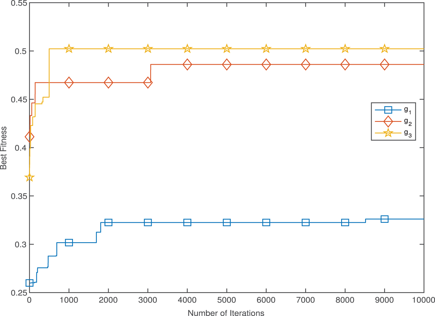
Figure 1 displays the convergence curves of the goal function by invoking g1, g2 and g3. As the iteration increases, PS2 (based on g2) converges faster than PS1 and PS3. Furthermore, since the partial similarity of the portfolio with the priori return based on g2 is greater than the other than the other partial similarity measures based on g1 and g3, we prefer the partial similarity measure (PS2) to optimize any similar portfolio selection model.
Convergence curve of different similarity measures.
Conclusions
This paper proposed a new definition of partial similarity measure for uncertain random variables. Based on this definition, several properties of this concept were derived. Theoretically, the results in this paper extend the existing results in [19]. As an application, we planed to investigate portfolio selection of uncertain random variables involving uncertain factors(new markets) and under control random variables (historical markets) via mean-variance constraint model. As a future work, we can optimize portfolio selection of uncertain random returns based on partial similarity measure as a goal function and other types of constraints such as skewness, entropy and expectation. Also, future researches will cover the applications of similarity measure of uncertain random variables in the fields of image compression, clustering analysis, uncertain machine scheduling problem and so on.
Footnotes
Acknowledgments
This work was supported by the Natural Science Foundation of Hebei Province (No. F2020202056) and Key Project of Hebei Education Department (No. ZD2020125). The authors wish to thank the Editor-in-Chief, Associate Editor and anonymous referees for their constructive comments and insightful suggestions that aided in the improvement of this article. All computations were carried out by MATLAB R2015a in Windows Server 2016 Standard of desktop PC machine with Intel(R) Xeon(R) CPU E7-8890 v4 @ 2.20GHz, 2195 MHz, 24 Core(s), 24 Logical Processor(s) and 16.0 GB RAM. The computer program is available from the third author upon request.
References
1.
AhmadzadeH., GaoR., Covariance of uncertain random variables and its application to portfolio optimization, Journal of Intelligent and Fuzzy Systems https://doi.org/10.1007/s12652-019-01323-0.
2.
AhmadzadeH., GaoR., NaderiH. and FarahikiaM., Partial divergence measure of uncertain random variables and its application, Soft Computing24(1) (2020), 501–512.
3.
AhmadzadeH., GaoR., DehghanM.H. and ShengY., Partial Entropy of Uncertain Random Variables, Journal of Intelligent and Fuzzy Systems33 (2017), 105–112.
4.
AhmadzadeH., GaoR. and ZareiH., Partial Quadratic Entropy of Uncertain Random Variables, Journal of Uncertain Systems10(4) (2016), 292–301.
5.
AhmadzadeH., ShengY.H. and Hassantabar DarziF., Some results of moments of uncertain random variables, Iranian Journal of Fuzzy Systems14(2) (2017), 1–21.
6.
AskarzadehA., A novel metaheuristic method for solving constrained engineering optimization problems: Crow search algorithm, Computers and Structures169(1) (2016), 1–12.
7.
CapitaineH., A relevance-based learning model of fuzzy similarity measures, IEEE Transactions on Fuzzy Systems20 (2012), 57–68.
8.
ChenX.W., KarS. and RalescuD.A., Cross-entropy measure of uncertain variables, Information Sciences201 (2012), 53–60.
9.
ChenS., Similarity measure between vague sets and between elements, IEEE Transactions on Systems Man Cybernetics27 (1997), 153–158.
10.
ChenS., MaB. and ZhangK., On the similarity metric and the distance metric, Theoretical Computer Science410 (2009), 2365–2376.
11.
ChouC., A new similarity measure of fuzzy numbers, Journal of Intelligent and Fuzzy Systems26 (2014), 287294.
12.
GaoX., JiaL. and KarS., A new definition of cross-entropy for uncertain variables, Soft Computing22 (2018), 5617–5623.
13.
HollandJ., Adaptation in natural and artificial systems, Ann Anbor: University of Michigan Press (1975).
14.
HouY.C., Subadditivity of Chance Measure, Journal of Uncertainty Analysis and Applications2(14) (2014), 1–8.
15.
KennedyJ. and EberhartR.C., Particle swarm optimization, Proc of IEEE International Conference on Neural Networks, Piscataway, (1995), 42–48.
16.
LiY., OlsonD. and QinZ., Similarity measures between intuitionistic fuzzy (vague) sets: A comparative analysis, Pattern Recognition Letters28 (2007), 278–285.
17.
LiD. and ChengC., New similarity measures of intuitionistic fuzzy sets and application to pattern recognition, Pattern Recognition Letters23 (2002), 221–225.
18.
LiX. and LiuB., On distance between fuzzy variables, Journal of Intelligent and Fuzzy Systems19 (2008), 197–204.
19.
LiX. and LiuY., Distance and similarity measures between uncertain variables, Journal of Intelligent and Fuzzy Systems28(5) (2015), 2073–2081.
LiuB., Some research problems in uncertainty theory, Journal of Uncertain Systems3(1) (2009), 3–10.
22.
LiuY.H. and HaM.H., Expected value of function of uncertain variables, Journal of Uncertain Systems4(3) (2010), 181–186.
23.
LiuY.H., Uncertain random variables: a mixture of uncertainty and randomness, Soft Computing17(4) (2013), 625–634.
24.
LiuY.H., Uncertain random programming with applications, Fuzzy Optimization and Decision Making12(2) (2013), 153–169.
25.
MajumdarP. and SamantaS., On similarity and entropy of neutrosophic sets, Journal of Intelligent and Fuzzy Systems26 (2014), 1245–1252.
26.
PengZ.X. and IwamuraK., A sufficient and necessary condition of uncertainty distribution, Journal of Interdisciplinary Mathematics13(3) (2010), 277–285.
27.
RezaeiK. and RezaeiH., New distance and similarity measures for hesitant fuzzy soft sets, Iranian Journal of Fuzzy Systems DOI: 10.22111/IJFS.2019.4571
28.
WangX. and DongC., Improving generalization of fuzzy ifthen rules by maximizing fuzzy entropy, IEEE Transactions on Fuzzy Systems17 (2009), 556–567.
29.
YangX.S. and DebS., Cuckoo search via Levy flights. In: Proceedings of World Congress on Nature and Biologically Inspired Computing (NaBIC), Coimbatore, India, 2009.
30.
YangX.S., Firefly algorithm, stochastic test functions and design optimisation, Int J Bio Inspired Comput2(2) (2010), 78–84.
31.
ZwickR., CarlsteinE. and BudescuD., Measures of similarity among fuzzy sets: A comparative analysis, International Journal of Aproximat Reasoning1 (1987), 221–242.