A novel semi-supervised method for classification of power quality disturbance using generative adversarial network

Abstract

The existing methods for classification of power quality disturbance signals (PQDs) have the problems that the process of signal feature selection is tedious and imprecise, the accuracy of classification has no guiding significance for feature extraction, and lack of adequate labelled training data. To solve these problems, this paper proposes a new semi-supervised method for classification of PQDs based on generative adversarial network (GAN). Firstly, a GAN model is designed which we call it PQDGAN. After the unsupervised pre-training with unlabeled training data, the trained discriminator is extracted alone and conduct supervised training with a small amount of labelled training data. Finally, the discriminator became a classifier with high accuracy. This model can achieve the step of feature extraction and selection efficiently. In addition, only a small amount of labelled training data is used, which greatly reduces the dependence of classification model on labelled data. Experiments show that this method has high classification accuracy, less computations and strong robustness. It is a new semi-supervised method for classification of PQDs.

Keywords

Deep learning generative adversarial network power quality semi-supervised learning signal classification.

1 Introduction

Due to the continuous development of society, the development of multi-energy integration has received more and more attention. Microgrid is one of the forms of multiple energy combinations. With the access of wind energy, solar energy and more non-linear load devices, the number of interference sources increases, resulting the microgrids are easier cause disturbance problem than the traditional grids [1]. To control power quality disturbance issue and take effective measures, the important step is to classify the types of PQDs accurately [2].

In order to classify the PQDs, researchers have proposed a variety of traditional methods, which can be roughly divided into three steps: feature extraction, feature selection, and feature classification [3]. In the step of feature extraction, many signal processing methods are used in this area, like Fourier Transform (FT), Empirical Mode Decomposition (EMD) [4], Short-Time Fourier Transform (STFT) [5, 6], Wavelet Transform (WT) [7], S-Transform (ST) [8, 9], Hilbert-Huang Transform (HHT) [10] and other methods which can obtain features from time domain and frequency domain of signals. But above these approaches are prone to be affected by the noise signal and have a heavy computation burden [13]. Therefore, a new feature extraction algorithm with less computations and strong anti-noise capability should be adopted.

In previous studies, the step of feature selection, whether quantities or types, relied mainly on manual operations. In order to choose the features more objectively, the researchers have used some intelligent algorithms to exclude the redundant features and extract the optimal features for classification, such as the artificial bee colony algorithm in [11] to select the optimal features of the perturbation classification. In [12], the authors used the sequential backward selection (SBS) as wrapper to select the most useful feature subset. In [13], the adaptive probabilistic neural network was used as the global optimization algorithm to gradually remove the redundant and irrelevant features in the noisy environment. But no matter what method is employed, the step of feature selection is time consuming and cumbersome, adding computational cost to the entire classification process. There should be a more efficient method to achieve feature selection and eliminating manual operation.

The classifiers used by the traditional PQDs classification method mainly include artificial neural network (ANN) [14, 15], decision trees (DT) [16], and support vector machine (SVM) [17] and other smart technologies. However, since the traditional PQDs classification process is not a closed loop process, the feature extraction and classification are separate, which means the accuracy of classification has no guiding significance for feature extraction.

Fortunately, Hinton presented deep learning in 2006. Deep learning is a kind of representation learning, that allows a deep neural network input original data and then extract features needed for classification automatically, which is efficient and can eliminate manual operation. Meanwhile, it makes the process of PQDs classification become a unified whole, which means the accuracy of classification result has guidance on the feature extraction. The deep belief networks (DBN) was used to achieve automatic feature extraction and selection in [18], but this method needs to normalize signals into the interval [0,1], and the number of types distinguished is small. In [36], researchers used wigner-ville distribution (WVD) technology to transfer a 1D voltage disturbance signal into a 2D image file, followed by a convolutional neural network (CNN) model developed for the image classification. The classification accuracy is high but the pre-processing is complicated, and the number of experimental types of PQDs is small. In [19], an end-to-end classifier based on deep CNN (DCNN) is proposed. The whole model is a closed-loop system without signal pre-processing. Compared with traditional methods, the classification process is simpler.

The above classification method based on DCNN adopts a large number of labelled data set for training. However, for many machine learning tasks, the cost of collecting labelled data is expensive because it involves relevant expertise inevitably. In contrast, it is much easier and cheaper to obtain unlabeled data [20]. In terms of PQDs classification, most power system monitors cannot give PQDs type. They only store historical waveform data without disturbance type label. So, it is very difficult to apply the deep learning method based on supervised learning in the absence of labelled data. In [21], multiple k nearest neighbor (KNN)-based regularized binary classifiers are adopted as semi-supervised model to classify PQDs, and the labelled data is only a small part of the training data set. However, the classification process is too complex, and it doesn’t have the advantage of deep learning methods.

Given the comprehensive analysis of the advantages and disadvantages of the above PQDs classification methods, a novel semi-supervised deep learning method for classification of PQDs is proposed in this paper. The main contributions of this paper are as follows: we designed a deep learning model based on GAN, which we call it PQDGAN. It consists of generator and discriminator, and the training process include two parts: unsupervised pre-training and supervised training. After all the training process, we can get an end-to-end classifier with high accuracy. Compare with above methods, our deep learning model has a simple structure, and can learn extract features automatically. The training data set contains a small amount of labelled data, which greatly reduces the dependence on labelled data. As far as we know, this is the first time to apply GAN model to the PQDs classification field.

This paper is structured as follows: Section 2 introduces the PQDs problem and its mathematical models. In Section 3, the PQDGAN model is proposed. Section 4 carries out experiments and Section 5 concludes and summarizes our work roundly.

2 PQDs problem and its mathematical model

2.1 The produce of PQDs

PQDs refer to the deviation of voltage, current and frequency from standard rating. With the proposed of smart grid, the electric energy converted from other energy sources is connected to the power grid successively, such as the electric energy generated by solar power generation, wind power generation and other new energy sources. This will not only help to coordinate energy sources more efficiently, but also reduce carbon emissions. However, due to the obvious volatility, randomness and intermittency of energy sources such as solar energy and wind energy [11], the voltage generated is prone to fluctuation. And with addition of phev smart charging station and other electronic devices, the entire power grid became more complex, which makes PQDs are easier to produce in the power grid [22]. In order to reduce the property loss and personnel risk caused by the PQDs problem, researchers have paid more and more attention to this aspect in recent years. How to identify various single PQDs and multiple PQDs accurately and rapidly is still a challenge.

2.2 Mathematical models of PQDs

Following [19], we get 16 mathematical models of PQDs. The 16 types include 10 single types like pure sine waveforms, sag, swell, interruption, harmonics, impulsive transients, oscillation transients, flicker, periodic notch, spikes and 6 multiple types like sag with harmonics, swell with harmonics, interruption with harmonics, flicker with harmonics, flicker with sag, flicker with swell. The parameter changes comply with ieee-1159 standard [23], mathematical models are shown in Table 1.

Table 1
Mathematical models of PQDs

PQDs Mathematical equations Parameters

Normal y (t) = A [1 ± α (u (t - t₁) - u (t - t₂))] sin(ωt) α ⩽ 0.1 T ⩽ t₂ - t₁ ⩽ 9T

Sag y (t) = A [1 - α (u (t - t₁) - u (t - t₂))] sin(ωt) 0.1 ⩽ α ⩽ 0.9 T ⩽ t₂ - t₁ ⩽ 9T

Swell y (t) = A [1 + α (u (t - t₁) - u (t - t₂))] sin(ωt) 0.1 ⩽ α ⩽ 0.8 T ⩽ t₂ - t₁ ⩽ 9T

Interruption y (t) = A [1 - α (u (t - t₁) - u (t - t₂))] sin(ωt) 0.9 ⩽ α ⩽ 1 T ⩽ t₂ - t₁ ⩽ 9T

Harmonics y (t) = A [α₁ sin(ωt) + α₃ sin(3ωt) + α₅ sin(5ωt) + α₇ sin(7ωt)] 0.05 ⩽ α₃, α₅, α₇ ⩽ 0.15 $\sum α_{i}^{2} = 1$

Impulsive transients y (t) = A [1 - α { u (t - t₁) - u (t - t₂) }] sin(ωt) 0 ⩽ α_i ⩽ 0.414 T/20 ⩽ t₂ - t₁ ⩽ T/10

Oscillation transients $y (t) = A [sin (ω t) + α^{- \frac{c (t - t_{1})}{τ}} sin ω_{n} (t - t_{1}) (u (t_{2}) - u (t_{1}))]$ 0.1 ⩽ α ⩽ 0.8 0.5T ⩽ t₂ - t₁ ⩽ 3T 8ms ⩽ τ ⩽ 40ms 300 ⩽ f_n ⩽ 900Hz

Flicker y (t) = A [1 + α_f sin(βωt)] sin(ωt) 0.1 ⩽ α_f ⩽ 0.2 5 ⩽ β ⩽ 20Hz

Periodic notch $y (t) = sin (ω t) - sign (sin (ω t)) \times {\sum_{n = 0}^{9} κ [u (t - (t_{1} - 0.02 n)) - u (t - (t_{2} - 0.02 n))]}$ 0 ⩽ t₁, t₂ ⩽ 0.5T 0.01T ⩽ t₂ - t₁ ⩽ 0.05T

0.1 ⩽ κ ⩽ 0.4

Spikes $y (t) = sin (ω t) + sign (sin (ω t)) \times {\sum_{n = 0}^{9} κ [u (t - (t_{1} - 0.02 n)) - u (t - (t_{2} - 0.02 n))]}$ 0 ⩽ t₁, t₂ ⩽ 0.5T 0.01T ⩽ t₂ - t₁ ⩽ 0.05T

0.1 ⩽ κ ⩽ 0.4

Sag with harmonic y (t) = A [1 - α (u (t - t₁) - u (t - t₂))] [α₁ sin(ωt) + α₃ sin(3ωt) + α₅ sin(5ωt)] 0.1 ⩽ α ⩽ 0.9 T ⩽ t₂ - t₁ ⩽ 9T 0.05 ⩽ α₃, α₅, α₇ ⩽ 0.15 $\sum α_{i}^{2} = 1$

Swell with harmonics y (t) = A [1 + α (u (t - t₁) - u (t - t₂))] [α₁ sin(ωt) + α₃ sin(3ωt) + α₅ sin(5ωt)] 0.1 ⩽ α ⩽ 0.8 T ⩽ t₂ - t₁ ⩽ 9T 0.05 ⩽ α₃, α₅, α₇ ⩽ 0.15 $\sum α_{i}^{2} = 1$

Interruption with harmonics y (t) = A [1 - α { u (t - t₁) - u (t - t₂) }] [α₁ sin(ωt) + α₃ sin(3ωt) + α₅ sin(5ωt)] 0.9 ⩽ α ⩽ 1 T ⩽ t₂ - t₁ ⩽ 9T 0.05 ⩽ α₃, α₅, α₇ ⩽ 0.15 $\sum α_{i}^{2} = 1$

Flicker with harmonics y (t) = A [1 + α_f sin(βωt)] sin(ωt) [α₁ sin(ωt) + α₃ sin(3ωt) + α₅ sin(5ωt)] 0.1 ⩽ α_f ⩽ 0.2 5 ⩽ β ⩽ 20Hz 0.05 ⩽ α₃, α₅, α₇ ⩽ 0.15 $\sum α_{i}^{2} = 1$

Flicker with sag y (t) = A [1 + α_f sin(βωt)] sin(ωt) (1 - α (u (t - t₁) - u (t - t₂))) 0.1 ⩽ α ⩽ 0.9 T ⩽ t₂ - t₁ ⩽ 9T 0.1 ⩽ α_f ⩽ 0.2 5 ⩽ β ⩽ 20Hz

Flicker with swell y (t) = A [1 + α_f sin(βωt)] sin(ωt) (1 + α (u (t - t₁) - u (t - t₂))) 0.1 ⩽ α ⩽ 0.8 T ⩽ t₂ - t₁ ⩽ 9T 0.1 ⩽ α_f ⩽ 0.2 5 ⩽ β ⩽ 20Hz

PQDs	Mathematical equations	Parameters
Normal	y (t) = A [1 ± α (u (t - t₁) - u (t - t₂))] sin(ωt)	α ⩽ 0.1 T ⩽ t₂ - t₁ ⩽ 9T
Sag	y (t) = A [1 - α (u (t - t₁) - u (t - t₂))] sin(ωt)	0.1 ⩽ α ⩽ 0.9 T ⩽ t₂ - t₁ ⩽ 9T
Swell	y (t) = A [1 + α (u (t - t₁) - u (t - t₂))] sin(ωt)	0.1 ⩽ α ⩽ 0.8 T ⩽ t₂ - t₁ ⩽ 9T
Interruption	y (t) = A [1 - α (u (t - t₁) - u (t - t₂))] sin(ωt)	0.9 ⩽ α ⩽ 1 T ⩽ t₂ - t₁ ⩽ 9T
Harmonics	y (t) = A [α₁ sin(ωt) + α₃ sin(3ωt) + α₅ sin(5ωt) + α₇ sin(7ωt)]	0.05 ⩽ α₃, α₅, α₇ ⩽ 0.15 $\sum α_{i}^{2} = 1$
Impulsive transients	y (t) = A [1 - α { u (t - t₁) - u (t - t₂) }] sin(ωt)	0 ⩽ α_i ⩽ 0.414 T/20 ⩽ t₂ - t₁ ⩽ T/10
Oscillation transients	$y (t) = A [sin (ω t) + α^{- \frac{c (t - t_{1})}{τ}} sin ω_{n} (t - t_{1}) (u (t_{2}) - u (t_{1}))]$	0.1 ⩽ α ⩽ 0.8 0.5T ⩽ t₂ - t₁ ⩽ 3T 8ms ⩽ τ ⩽ 40ms 300 ⩽ f_n ⩽ 900Hz
Flicker	y (t) = A [1 + α_f sin(βωt)] sin(ωt)	0.1 ⩽ α_f ⩽ 0.2 5 ⩽ β ⩽ 20Hz
Periodic notch	$y (t) = sin (ω t) - sign (sin (ω t)) \times {\sum_{n = 0}^{9} κ [u (t - (t_{1} - 0.02 n)) - u (t - (t_{2} - 0.02 n))]}$	0 ⩽ t₁, t₂ ⩽ 0.5T 0.01T ⩽ t₂ - t₁ ⩽ 0.05T
		0.1 ⩽ κ ⩽ 0.4
Spikes	$y (t) = sin (ω t) + sign (sin (ω t)) \times {\sum_{n = 0}^{9} κ [u (t - (t_{1} - 0.02 n)) - u (t - (t_{2} - 0.02 n))]}$	0 ⩽ t₁, t₂ ⩽ 0.5T 0.01T ⩽ t₂ - t₁ ⩽ 0.05T
		0.1 ⩽ κ ⩽ 0.4
Sag with harmonic	y (t) = A [1 - α (u (t - t₁) - u (t - t₂))] [α₁ sin(ωt) + α₃ sin(3ωt) + α₅ sin(5ωt)]	0.1 ⩽ α ⩽ 0.9 T ⩽ t₂ - t₁ ⩽ 9T 0.05 ⩽ α₃, α₅, α₇ ⩽ 0.15 $\sum α_{i}^{2} = 1$
Swell with harmonics	y (t) = A [1 + α (u (t - t₁) - u (t - t₂))] [α₁ sin(ωt) + α₃ sin(3ωt) + α₅ sin(5ωt)]	0.1 ⩽ α ⩽ 0.8 T ⩽ t₂ - t₁ ⩽ 9T 0.05 ⩽ α₃, α₅, α₇ ⩽ 0.15 $\sum α_{i}^{2} = 1$
Interruption with harmonics	y (t) = A [1 - α { u (t - t₁) - u (t - t₂) }] [α₁ sin(ωt) + α₃ sin(3ωt) + α₅ sin(5ωt)]	0.9 ⩽ α ⩽ 1 T ⩽ t₂ - t₁ ⩽ 9T 0.05 ⩽ α₃, α₅, α₇ ⩽ 0.15 $\sum α_{i}^{2} = 1$
Flicker with harmonics	y (t) = A [1 + α_f sin(βωt)] sin(ωt) [α₁ sin(ωt) + α₃ sin(3ωt) + α₅ sin(5ωt)]	0.1 ⩽ α_f ⩽ 0.2 5 ⩽ β ⩽ 20Hz 0.05 ⩽ α₃, α₅, α₇ ⩽ 0.15 $\sum α_{i}^{2} = 1$
Flicker with sag	y (t) = A [1 + α_f sin(βωt)] sin(ωt) (1 - α (u (t - t₁) - u (t - t₂)))	0.1 ⩽ α ⩽ 0.9 T ⩽ t₂ - t₁ ⩽ 9T 0.1 ⩽ α_f ⩽ 0.2 5 ⩽ β ⩽ 20Hz
Flicker with swell	y (t) = A [1 + α_f sin(βωt)] sin(ωt) (1 + α (u (t - t₁) - u (t - t₂)))	0.1 ⩽ α ⩽ 0.8 T ⩽ t₂ - t₁ ⩽ 9T 0.1 ⩽ α_f ⩽ 0.2 5 ⩽ β ⩽ 20Hz

The simulated PQDs waveforms using mathematical models are shown in Fig. 1. According to the formula shown in Table 1, we used MATLAB R2016a to generate the training data set and test data set. Different samples can be obtained by changing the parameters within the appropriate range.

Fig. 1

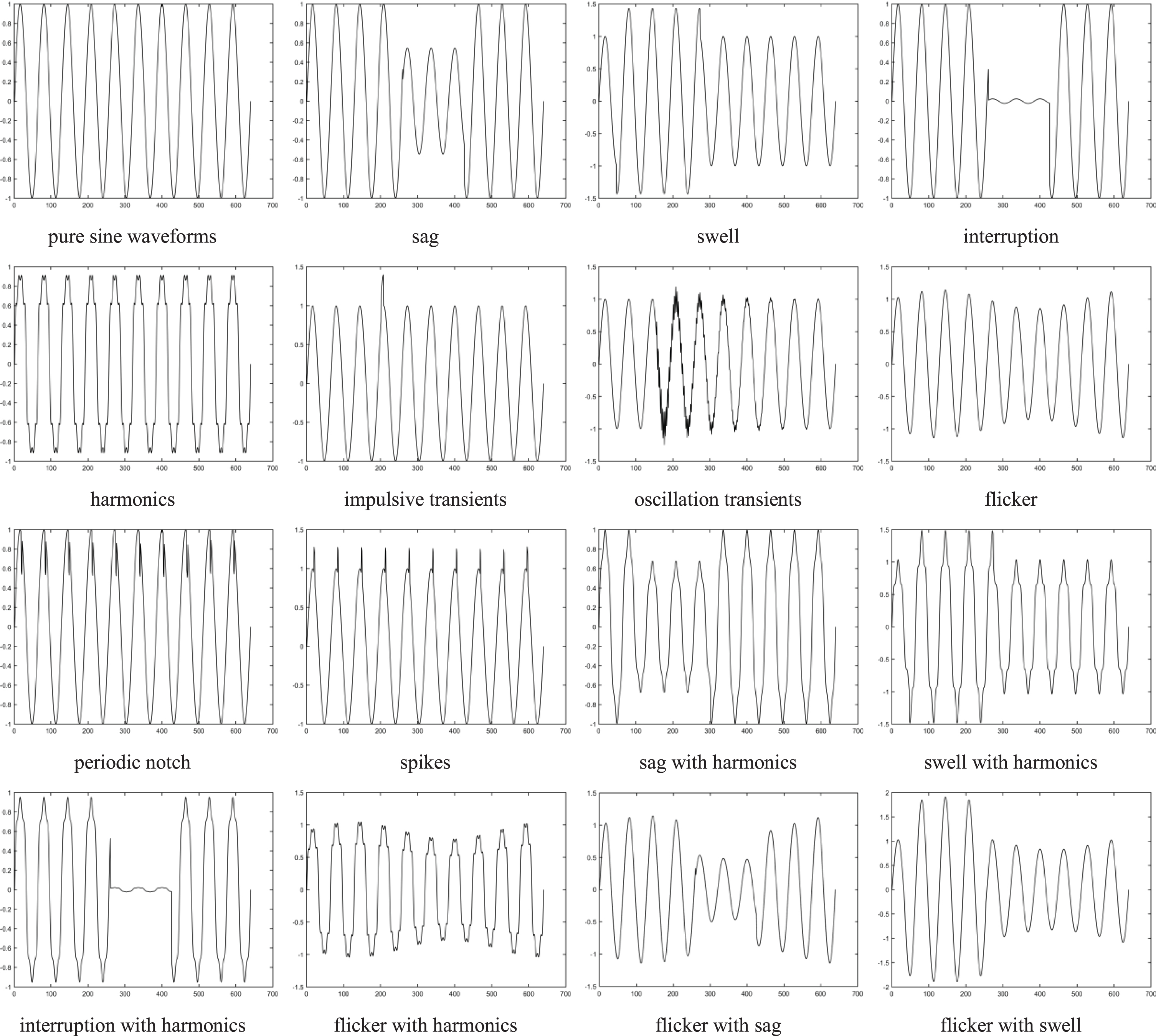
The waveforms of PQDs.

The sampling frequency of 3.2 kHz is adopted, which is commonly used in power equipment. And 640 points of each sample are collected as sampling points in ten cycles total 0.2 seconds. For each type, 6,400 unlabeled samples and 30 labelled samples are randomly generated, totaling 102,400 unlabeled samples and 480 labelled samples are used for training. 1,000 labelled samples are randomly generated for testing for each type, the number of test set has reached 16,000. The label data is represented by one hot encoding like {1,0,0,0,0,0,0,0,0,0,0,0,0,0,0,0} (it means the sample belongs to first category), to facilitate the computation of loss function.

This section describes the produce of PQDs and its mathematical model. According to its mathematical model, we made training data set and test data set to provide samples for experiments in the following sections.

3 PQDGAN classification model design

3.1 Original GAN model

GAN is a deep learning network structure that was proposed in 2014 [24] and is widely used in image generation [25], image fusion [26], image translation [27], test-to-image [28]. In terms of classification, it is applied to URL classification [29] and classification of BSR (buzz, squeak, and rattle) noises [30]. At present, GAN model has become one of the most important models in the field of deep learning.

The original GAN model consists of two parts: generator (G) which generates fake samples close to the real samples with random noise z and discriminator (D) which determines whether the samples are from the real samples or the fake samples. These two nets are against each other. G tries to fool D by generating fake samples that are close to the true sample, while D tries to learn how to identify true and fake samples as much as possible. And in the process of fighting each other, they become better than the previous iteration.

The against loss function for the G is defined as: $L_{G} = - E_{z \sim p_{z} (z)} [- log (1 - D (G (z)))]$ (1) the against loss function for the D is defined as:

$\begin{matrix} L_{D} = - E_{x \sim p_{data} (x)} \\ [- log (D (x))] + E_{z \sim p_{z} (z)} [- log (1 - D (G (z)))] \end{matrix}$ (2) where p_data (x) and p_z (z) are the training data distribution and random noise distribution, respectively. x denotes the real sample and G (z) denotes the fake sample generated by G. After the training, G (z) will be similar to x, and D is unable to differentiate between the two samples.

3.2 PQDGAN design

We referred two GAN variants: deep convolutional GAN(DCGAN) [31] and wasserstein GAN with gradient punishment (WGAN-GP) [32]. Inspired by the structure of DCGAN and against loss function of WGAN-GP, we designed PQDGAN model. Compare with original GAN model, the main changes of PQDGAN model are as follows:

Hidden layer in the network structure of G and D is constituted by one-dimensional convolution layer, which allows the network to process one-dimensional signals.

Use ReLU activation function in G for all layers except for the output, which uses Tanh. Use LeakyReLU activation function in the D for all layers except for the output, which depends on the training phase. These changes of activation function allowed the model to learn more quickly to saturate.

Against loss function with gradient penalty of WGAN-GP was adopted, which can make the whole model more stable, reduce the risk of mode collapse of original GAN and accelerate the convergence. It is also beneficial to the following classification training.

BN layer is not used in G and D in unsupervised training process to prevent impact on gradient punishment in against loss function.

The framework of PQDGAN model is shown in Fig. 2. As shown in Fig. 2, our model consists of G net and D net. The whole training process include two phases: unsupervised pre-training and supervised training. In unsupervised pre-training, the input of G net is random noise z and the output is fake sample G (z). The input of D net is fake sample G (z) or unlabeled real data x and the output is a single scalar denoting whether the input is “real” or “fake”. The loss function is against loss function. In supervised training, D classifies the labelled data x to n-class and loss function is Softmax loss function.

Fig. 2

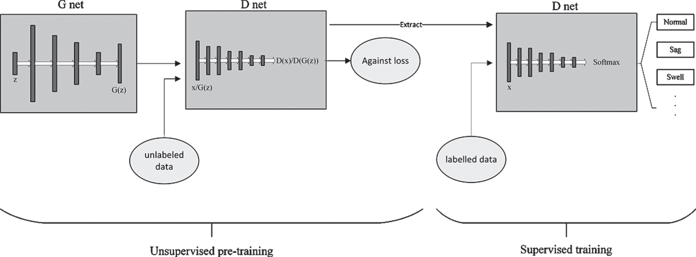
The framework of PQDGAN.

In order to understand the training process better, the training procedure is summarized in the provided pseudo-code (Algorithm 1 and Algorithm 2). In the Algorithm 1, G will learn the distribution of real unlabeled data, so as to generate fake samples. D will learn how to extract features form unlabeled data. They compete against each other to improve performance. Then we save the parameters of D and replacing the sigmoid activation function with Softmax in the last layer. Then we do the next phase training. In the Algorithm 2, we train D with a small number of labelled data set alone. Each parameter will be updated automatically by the feedback of classification performance (descending Softmax loss function). After the whole training process, we can get D as classifier with high accuracy.

Algorithm 1: Unsupervised pre-training Algorithm
Require: random noise samples, unlabeled train data set,
b is the number of batches, φ and θ the initial parameters
of G and D.
for number of training iterations do
Sample ${z^{(i)}}_{i = 1}^{b} \sim p_{z} (z)$ a batch of random
noise samples.
Sample ${x^{(i)}}_{i = 1}^{b} \sim p_{data} (x)$ a batch of
unlabeled train data set.
Random number ${u^{(i)}}_{i = 1}^{b} \sim U [0, 1]$ .
Generate fake sample ${G {(z)}^{(i)}}_{i = 1}^{b}$ .
Update θ from D by descending L_WD.
Update φ from G by descending L_WG.
end for

Algorithm 2: Supervised training Algorithm
Require: labelled train data set, b is the number of
batches, θ the pre-training parameters of D.
for number of training iterations do
Sample ${x^{(i)}}_{i = 1}^{b} \sim p_{data} (x)$ a batch of
labelled train data set.
Sample corresponding real label ${y^{(i)}}_{i = 1}^{b}$ .
Get predict label ${{\hat{y}}^{(i)}}_{i = 1}^{b} = D ({x^{(i)}}_{i = 1}^{b})$ .
Update θ from D by descending L_softmax.
end for

The against loss function in unsupervised pre-training is: $\begin{matrix} L_{WD} = - E_{x \sim p_{data} (x)} + E_{z \sim p_{z} (z)} [D (G (z))] \\ + λ E_{\hat{x} \sim p_{\hat{x}}} [\nabla_{\hat{x}} D {(\hat{x})}_{2} - 1]^{2} \end{matrix}$ (3) $L_{WG} = - E_{z \sim p_{z} (z)} [D (G (z))]$ (4) where x is real sample, G (z) is fake sample generated by G, $\hat{x} = u * x + (1 - u) * G (z)$ , u is random number between [0,1], and λ is used to strike a balance between against loss and gradient punishment. Compare with against loss function of original GAN (Equations (1) and (2)), gradient punishment is added to make the gradient more stable in the training process.

The loss function in supervised training is: $L_{softmax} = - \sum_{i = 1}^{n} y_{i} \log {\hat{y}}_{i}$ (5) where y is the real label of sample and $\hat{y}$ is the predict label, they are one hot encoding. n is the number of classifications.

In order to determine the parameters which are suitable for PQDs classification, we explored the influence of different convolution kernel sizes on model performance. The convolution kernel sizes in G and D networks adopt 1×3, 1×5 and 1×7 respectively. We trained the model and recorded the best accuracy. We refer to [32] to set up training details include iteration batches, parameters of Adam optimizer, gradient punishment parameter λ and learning rate. The training details are shown in Table 2. The training set and test set are from Section 2.2. The results are shown in Table 3.

Table 2

Training details

Iteration batches	64
Parameters of Adam optimizer	beta 1 = 0.5, beta 2 = 0.9
λ	10
Learning rate	0.0001

Table 3

Influence of different convolution kernel sizes on model performance

Kernel size of G	Kernel size of D	Number of unsupervised learning iterations	Best accuracy in test set (%)
1×3	1×3	22,400	98.29
	1×5	25,600	98.23
	1×7	32,000	98.69
1×5	1×3	32,000	98.36
	1×5	28,800	98.13
	1×7	25,600	98.78
1×7	1×3	25,600	98.13
	1×5	25,600	98.48
	1×7	28,800	98.64

According to Table 3, we determine that when the convolution kernel of G is 1×5 and convolution kernel of D is 1×7 can achieve the best classification accuracy. Third column is the number of unsupervised training iterations when we can get the best accuracy. After 25,600 unsupervised learning iterations, the accuracy can reach 98.78%. So, we get the most suitable network parameters for PQDs classification.

The parameters of each layer are shown in Table 4. In the G net, FC is the fully connected layer, which takes a random noise z as the 1-D input. The Upsampling layer denote deconvolution, which rescales the front layer to the desired size. In the D net, Conv layer denotes convolution layer and Lowsampling layer denotes convolution layer combined with strides to realize reducing-dimension processing. Output layer is a fully connected layer which can decide the size of output.

Table 4

PQDGAN model structure parameters

	Name of layer	Size of kernel	Strides	Feature map	Activation function
G net	Input	——	——	1×100	——
	FC	1×20480	——	1×20480	ReLU
	Reshape	——	——	1×160×128	——
	Upsampling	1×5×64	1×2	1×320×64	ReLU
	Upsampling	1×5×32	1×1	1×320×32	ReLU
	Upsampling/Output	1×5×1	1×2	1×640×1	Tanh
D net	Input	——	——	1×640×1	——
	Conv	1×7×32	1×1	1×640×32	LeakyReLU
	Lowsampling	1×7×32	1×2	1×320×32	LeakyReLU
	Conv	1×7×64	1×1	1×320×64	LeakyReLU
	Lowsampling	1×7×64	1×2	1×160×64	LeakyReLU
	Conv	1×7×128	1×1	1×160×128	LeakyReLU
	Lowsampling	1×7×128	1×2	1×80×128	LeakyReLU
	Output	1×1	——	1×1	——
	Output	1×16	——	1×16	Softmax

To verify that D learned some features from unlabeled samples in unsupervised pre-training and against loss function adopted has an effect on the model performance, we established a D classifier without unsupervised pre-training which we call it CNN. We also established other two models: DCGAN and DCGAN+GP. DCGAN denote our model with the loss function of original GAN and DCGAN+GP denote our model with the loss function of WGAN-GP. The number of unsupervised pre-training iterations is set to 25600 and the number of supervised training iterations is set to 4000. The training details are shown in Table 2. The training set and test set are from Section 2.2. The changes of their classification accuracy curve are shown in Fig. 3.

Fig. 3

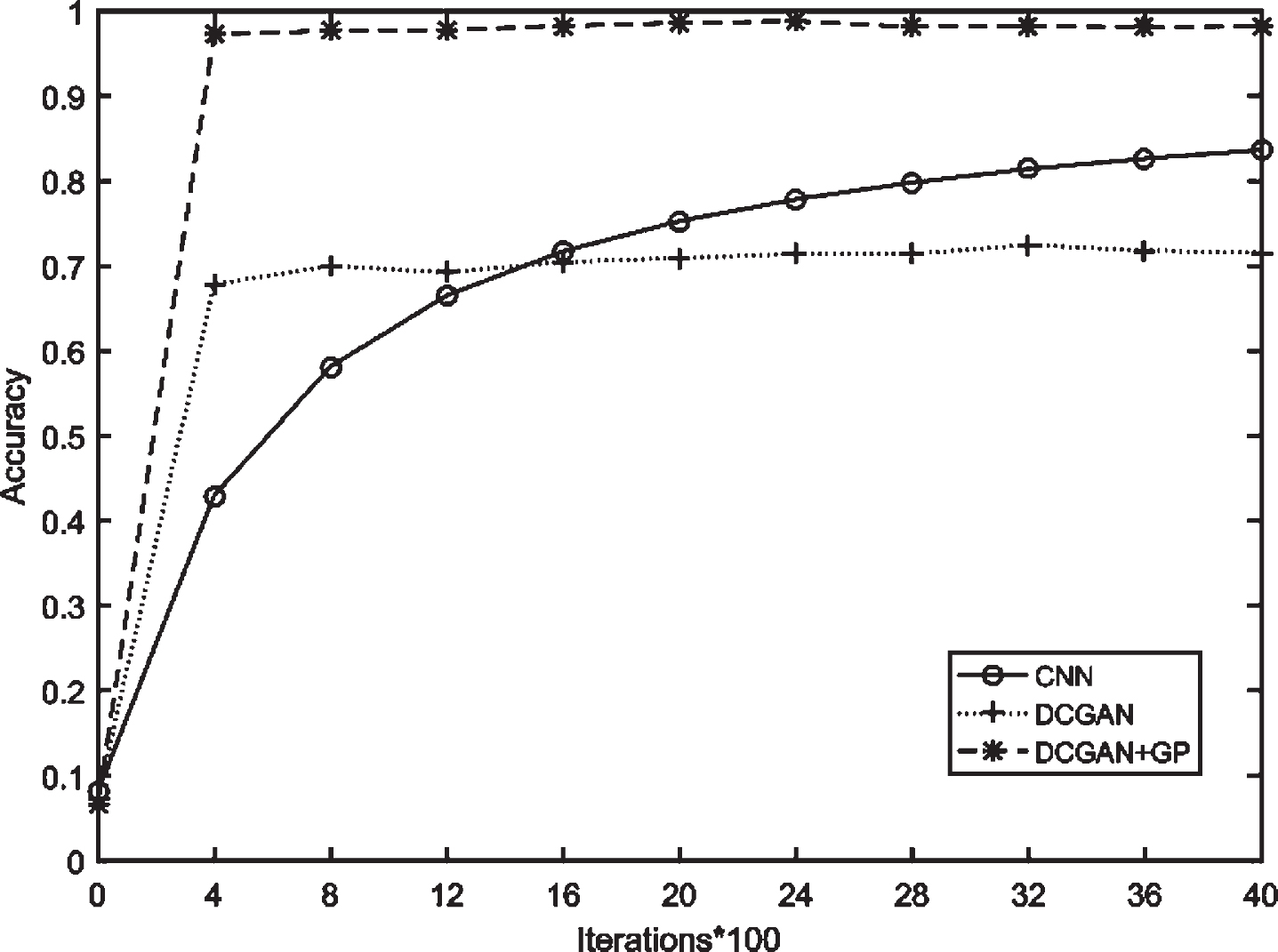
Classification accuracy curves of three models.

Fig. 3 shows that, after 4000 iterations of supervised learning, our model can reach a stable accuracy. The accuracy of DCGAN+GP is improved faster than CNN classifier. It means D learns some features from the unlabeled samples in unsupervised pre-training. Although, DCGAN can also reach the best accuracy fast, the accuracy is not high comparing with DCGAN+GP. Because the against loss function adopted in DCGAN+GP has a good effect on the model performance.

In this section, a deep learning model based on GAN has been designed to classify PQDs. The whole model training process includes two parts: unsupervised pre-training and supervised training. In training, the model can extract features automatically which are useful for classification. Our method can train a classifier with satisfactory accuracy under the rare of labelled data. So, it can reduce the dependence of classifiers on labelled data set.

4 Experimental and analysis

To emphasize the superiority of our method, PQDGAN is compared with DCNN classification model in [19] and ST+KNN classification model in [21]. DCNN classification model is a PQDs classification deep learning model based on the DCNN. Its network structure is mainly composed of convolutional layers, full connections layers and pooling layers. Signals can be classified without pre-processing. This model has higher classification accuracy and simpler structure compared with other PQDs classification deep learning models in [19]. ST+KNN classification model is a semi-supervised PQDs classification traditional model. ST is chosen to exaction of adequate time-frequency features of the PQDs. Then, features from unlabeled data and labelled data are used in building multiple KNN-based regularized binary classifiers. The model can achieve good performance under the rare of labelled data.

Firstly, we compare these three models in terms of training set, structure and number of iterations. The results are reported in Table 5.

Table 5
Comparison of classification methods

Model Number of labelled training data Number of unlabeled training data Total number of training data Structure of classifier model Number of iterations

DCNN 768000 0 768000 12-layer network (6 convolution layer +3 full connections layer +3 pooling layer) 840000

ST+KNN 30 470 500 n-knn based binclassifiers (n represents the number of individual types) ——

PQDGAN 480 102400 102880 7-layer network (6 convolution layer +1 full connection layer) 29600(25600 + 4000)

Model	Number of labelled training data	Number of unlabeled training data	Total number of training data	Structure of classifier model	Number of iterations
DCNN	768000	0	768000	12-layer network (6 convolution layer +3 full connections layer +3 pooling layer)	840000
ST+KNN	30	470	500	n-knn based binclassifiers (n represents the number of individual types)	——
PQDGAN	480	102400	102880	7-layer network (6 convolution layer +1 full connection layer)	29600(25600 + 4000)

As can be seen from Table 5, the number of labelled data set, the total number of data set and iteration times adopted by our method is much less than that of DCNN model, which indicate that the training cost of our model are low. Although the number of training data in ST+KNN method is smallest, it belongs to the traditional PQDs classification method and does not have the advantages of deep learning method. The model is too complex to be applied in practical engineering. By contrast, our method has the simplest structure among the three methods, which means it is easier to implement. A smaller model can be run on embedded devices more efficiently.

Then, we compare the accuracy of PQDGAN model, DCNN model and ST+KNN model in terms of performance. The accuracy of these three models are obtained through the experiment.

The experiment data are from Section 2.2. In order to make the experiment more consistent with the actual situation, the training set is randomly added with Gaussian white noise of 20 dB to 50 dB SNR, and the test set is added with Gaussian white noise of 20 dB, 30 dB and 40 dB SNR, respectively. The details of the experiment data are shown in Table 6.

Table 6

The details of the experiment data

Data set type	Number of labelled data set	Number of unlabeled data set	SNR
Training set	30×16 = 480	6400×16 = 102400	From 20 dB to 50 dB
Test set	1000×16 = 1600	0	0 dB,20 dB,30 dB,40 dB

In the experiment, the number of unsupervised pre-training iterations is set to 25,600, the number of supervised training is set to 4,000, and the training details are shown in Table 2. We use Tensorflow deep learning framework to write program and conduct training on NVidia GTX1080 12 G GPU to recording the best accuracy achieved in the supervised training process. Experimental results are shown in Table 7 and Fig. 4.

Table 7

Experimental accuracy of three classifier

Model	Number of single types	Nubmer of multiple types	Number of total types	Accuracy (test set noiseless) (%)
DCNN	10	6	16	99.96
ST+KNN	7	3	10	98.20
PQDGAN	7	3	10	99.70
	10	6	16	98.75

Fig. 4

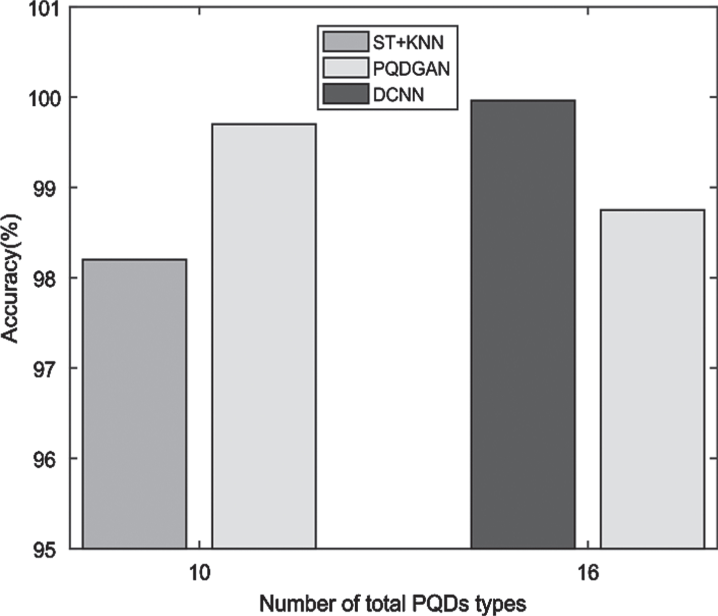
Classification accuracy of three models.

It can be seen from the Table 7 and Fig. 4 that, in the case of classifying the same 10 types of PQDs (seven single and three multiple PQDs, including pure sine, harmonics, flicker, sag, swell, interruption, oscillatory transients, sag with harmonic, swell with harmonic, flicker with harmonic and interruption with harmonic), the accuracy of our model is 99.7%, surpasses the ST+KNN classification model. In the case of classifying 16 types of PQDs (including all types of PQDs in Table 1), the accuracy of our model can reach 98.75%, which is in an acceptable range. But compared with DCNN model, our model has simpler structure, fewer training iterations, and less labelled data set for training, which eliminating manual tagging steps. It is more convenient to apply to practical engineering.

In terms of computational complexity, we compare the PQDGAN classifier and DCNN classifier because they belong to deep learning model. Their single sample classification time and multiply-accumulate operations (MACCs) are calculated respectively. Classification time represents the speed of model classification and MACCs represents how many multiply-accumulate computations model does. We only calculate the MACCs of convolution layer and full connection layer which account for the main computations in model. 1,000 samples are selected from the test set randomly to calculate average of classification time. The results are shown in Table 8.

Table 8

Computational complexity comparison results

Classifier	Classification time(s)	MACCs
DCNN	0.00229	81487827
PQDGAN	0.00164	46182400

As shown in Table 8, either classification time or MACCs, our classifier is less than DCNN classifier, which means our classifier is easier to run on embedded devices.

In order to test the robustness of the model, using test set which is added Gaussian white noise with 20 dB, 30 dB and 40 dB SNR to examine the performance of the classifier and observe its accuracy changes. See Table 9 for the experiment data.

Table 9

Changes in classification accuracy after adding noises with different SNR

SNR	0 dB	40 dB	30 dB	20 dB
Accuracy (%)	98.75	98.26	98.13	96.05

Table 9 shows that, although the accuracy of the model in this paper decreases after adding noise, it still maintained a good classification accuracy, which means the model has a strong robustness.

Additionally, a comparison of the proposed method with other methods is illustrated in Table 10, including five existing traditional PQDs classification methods, EMD with balanced neural tree (BNT) [33], empirical wavelet transform (EWT) with multiclass SVM [34], Hybrid ST with DT [13], ADALINE with fuzzy neural network (FNN) [35] and variational mode decomposition (VMD) with SVM [12]. The proposed method can extract feature automatically and achieve high accuracy. It shows that our method is more advantageous than other traditional PQDs classification methods.

Table 10

The comparison of the PQDGAN with other traditional PQDs classification methods

Method	Feature extraction	Number of PQDs	Accuracy (%)
EMD+BNT	Manual operation	8	97.90
EWT+multiclass SVM	Manual operation	16	95.56
Hybrid ST+DT	Manual operation	11	94.39
ADALINE+FNN	Manual operation	12	90.58
VMD+SVM	Manual operation	9	99.66
PQDGAN	Automatically	16	98.75

In this section, we compare our model with DCNN classification model and ST+KNN classification model in the term of in terms of training set, structure, number of iterations, classification accuracy and computational complexity. Experimental results show that our model has advantages in the above aspects. In addition, we also verify that our model has strong robustness and is more advantageous than traditional PQDs classification methods.

5 Summary and future works

In this paper, we propose a semi-supervised end-to-end model for classification of PQDs which we call it PQDGAN. This method solves the defects of previous PQDs classification methods that require manual feature selection and rely heavily on labelled data set. PQDGAN referred the structure of DCGAN and against loss function of WGAN-GP. It has simple structure and can automatically learn how to extract features from unlabeled data set, which make it more convenient to apply to practical engineering. Through experiments, the model showed high classification accuracy and little calculation. By adding Gaussian white noise to the data set, the model showed strong robustness. This paper provides a new idea for semi-supervised PQDs classification. In the future, we will explore the possibility of its hardware implementation.

References

Singh

G.K.

, Power system harmonics research: a survey, International Transactions on Electrical Energy Systems 19(1) (2009), 151–172.

Baggini

, Handbook of Power Quality, John Wiley & Sons (2008).

Mahela

O.P.

, Shaik

A.G.

and Gupta

, A critical review of detection and classification of power quality events, Renewable and Sustainable Energy Reviews 41 (2015), 495–505.

Manjula

, Mishra

and Sarma

A.V.R.S.

, Empirical mode decomposition with Hilbert transform for classification of voltage sag causes using probabilistic neural network, International Journal of Electrical Power & Energy Systems 44(1) (2013), 597–603.

Y.H.

and Bollen

M.H.J.

, Time-frequency and time-scale domain analysis of voltage disturbances, IEEE Transactions on Power Delivery 15(4) (2000), 1279–1284.

, Zhang

Y.Q.

, Li

Y.B.

and Fan

, Comparative study of STFT and S transform on detecting voltage sag, Power System Protection and Control 42(24) (2014), 44–48.

Moravej

, Abdoos

A.A.

and Pazoki

, Detection and Classification of Power Quality Disturbances Using Wavelet Transform and Support Vector Machines, Electric Machines & Power Systems 38(2) (2009), 182–196.

Jaya Bharata Reddya

, et al., Power quality analysis using Discrete Orthogonal S-transform (DOST), Digital Signal Processing 23(2) (2013), 616–626.

Dash

P.K.

, Panigrahi

B.K.

and Panda

, Power Quality Analysis Using S-Transform, IEEE Transactions on Power Delivery 18(2) (2003), 406–411.

10.

Tao

, et al., Classification of Power Quality Disturbance Signals Based on S-Transform and HHT, Proceedings of the 32nd Chinese Control Conference (2013), 26–28.

11.

Khokhar

, et al., A new optimal feature selection algorithm for classification of power quality disturbances using discrete wavelet transform and probabilistic neural network, Measurement 95 (2017), 246–259.

12.

Abdoos

A.A.

, et al., Combined VMD-SVM based feature selection method for classification of power quality events, Applied Soft Computing 38 (2016), 637–646.

13.

Biswal

and Dash

P.K.

, Detection and characterization of multiple power quality disturbances with a fast S-transform and decision tree based classifier, Digital Signal Processing 23(4) (2013), 1071–1083.

14.

Wijayakulasooriya

J.V.

, Putrus

G.A.

and Minns

P.D.

, Electric power quality disturbance classification using self-adapting artificial neural networks, IEE Proceedings-Generation, Transmission and Distribution 149(1) (2002), 98–101.

15.

Kanitpanyacharoean

and Premrudeepreechacharn

, Power quality problem classification using wavelet transformation and artificial neural networks, IEEE PES Power Systems Conference and Exposition (2004), 10–13.

16.

Kumar

, et al., Recognition of Power-Quality Disturbances Using S-Transform-Based ANN Classifier and Rule-Based Decision Tree, IEEE Transactions on Industry Applications 51(2) (2015), 1249–1258.

17.

Lin

W.-M.

, et al., Detection and Classification of Multiple Power-Quality Disturbances With Wavelet Multiclass SVM, IEEE Transactions on Power Delivery 23(4) (2008), 2575–2582.

18.

C.-M.

, et al., Classification of power-quality disturbances using deep belief network, 2018 International Conference on Wavelet Analysis and Pattern Recognition (ICWAPR), (2018), 15–18.

19.

Chen

and Wang

, A novel deep learning method for the classification of power quality disturbances using deep convolutional neural network, Applied Energy 235(1) (2019), 1126–1140.

20.

Berthelot

, et al., Mix Match: A Holistic Approach to Semi-Supervised Learning, arXiv preprint arXiv:1905.02249 [cs.LG], 2019.

21.

, et al., A novel method of complex PQ disturbances classification without adequate history data, 2016 IEEE Power and Energy Society General Meeting (PESGM) (2016), 17–21.

22.

van der Kam

and van Sark

, Smart charging of electric vehicles with photovoltaic power and vehicle-to-grid technology in a microgrid; a case study, Applied Energy 152(15) (2015), 20–30.

23.

Committee and Electric Machinery, IEEE Recommended Practice for Monitoring Electric Power Quality, IEEE Std 1159–2009 (Revision of IEEE Std 1159–1995), (2009).

24.

Goodfellow

, et al., Generative Adversarial Nets, Advances in Neural Information Processing Systems 27 (NIPS 2014) (2014).

25.

Bao

, et al., CVAE-GAN: Fine-Grained Image Generation through Asymmetric Training, IEEE International Conference on Computer Vision (ICCV) (2017), 2745–2754.

26.

, et al., FusionGAN: A generative adversarial network for infrared and visible image fusion, Information Fusion 48 (2019), 11–26.

27.

Armanious

, et al., MedGAN: Medical Image Translation using GANs, arXiv preprint arXiv:1806.06397[cs.CV], (2018).

28.

Zhang

, et al., StackGAN: Test to Photo-realistic Image Synthesis with Stacked Generative Adversarial Networks, IEEE International Conference on Computer Vision (2017), 5907–5915.

29.

Trevisan

and Drago

, Robust URL Classification With Generative Adversarial Networks, ACM SIGMETRICS Performance Evaluation Review 46(3) (2018), 143–146.

30.

Kim

J.-Y.

, Bu

S.-J.

and Cho

S.-B.

, Hybrid Deep Learning Based on GAN for Classifying BSR Noises from Invehicle Sensors, International Conference on Hybrid Artificial Intelligence Systems (2018), 27–38.

31.

Radford

, Metz

and Chintala

, Unsupervised Representation Learning with Deep Convolutional Generative Adversarial Networks, arXiv preprint arXiv:1511.06434 [cs.LG], (2016).

32.

Gulrajani

, et al., Improved Training ofWasserstein GANs, Neural Information Processing Systems (2017).

33.

Biswal

, Biswal

, Mishra

and Jalaja

, Automatic classification of power quality events using balanced neural tree, IEEE Transactions on Industrial Electronics 61(1) (2014), 521–530.

34.

Thirumala

, Pal

, Jain

and Umarikar

A.C.

, A classification method for multiple power quality disturbances using EWT based adaptive filtering and multiclass SVM, Neurocomputing 334 (2019), 265–274.

35.

Valtierra-Rodriguez

, de Jesus Romero-Troncoso

, Osornio-Rios

R.A.

and Garcia-Perez

, Detection and classification of single and combined power quality disturbances using neural networks, IEEE Transactions on Industrial Electronics 61(5) (2014), 2473–2482.

36.

Cai

, Cao

, Aarniovuori

, Pang

, Lin

and Li

, Classification of Power Quality Disturbances Using Wigner-Ville Distribution and Deep Convolutional Neural Networks, IEEE Access 7 (2019), 119099–119109.