
Abstract
The load forecasting is the significant task carried out by the electricity providing utility companies for estimating the future electricity load. The proper planning, scheduling, functioning, and maintenance of the power system rely on the accurate forecasting of the electricity load. In this paper, the clustering-based filter feature selection is proposed for assisting the forecasting models in improving the short term load forecasting performance. The Recurrent Neural Network based Long Short Term Memory (LSTM) is developed for forecasting the short term load and compared against Multilayer Perceptron (MLP), Radial Basis Function (RBF), Support Vector Regression (SVR) and Random Forest (RF). The performance of the forecasting model is improved by reducing the curse of dimensionality using filter feature selection such as Fast Correlation Based Filter (FCBF), Mutual Information (MI), and RReliefF. The clustering is utilized to group the similar load patterns and eliminate the outliers. The feature selection identifies the relevant features related to the load by taking samples from each cluster. To show the generality, the proposed model is experimented by using two different datasets from European countries. The result shows that the forecasting models with selected features produce better performance especially the LSTM with RReliefF outperformed other models.
Introduction
The forecasting of the short-term electricity load is a critical task for the electricity providing utility companies in their operation and management of the supply to their customers. The load forecasting plays a vital role in the power system for achieving power demand and supply equilibrium by proper power system planning, design, development, distribution, and maintenance. The inaccurate forecasting may create unfair financial implications for the power system [19]. The load forecasting is divided into three major categories namely, long-term load forecasting, medium-term load forecasting and short-term load forecasting. The forecasting done for the next one hour to one week is known as short-term load forecasting, the forecasting is done for the next one week to a month and next one month to a year is known as medium-term and long-term load forecasting respectively [52].The electricity cannot be generated in large scale excessively for satisfying the future electricity demand. So, it should be generated when there is a demand for it. If the demand for the load is known in advance, all the related operational requirements for the generation of the electricity are made available without any delay. The over estimation or an under estimation of the load leads to the complex financial implications to the power system [55]. From the application point of view, the short term load forecasting is important for the proper functioning, stable and an economic operation of the power system. It helps to make decision on the day-to-day operational activities such as proper planning and scheduling of power generation, scheduling of fuel purchase, allocation of resources, unit commitment, load increment and decrement, scheduling of maintenance, energy storage optimization and preparing the dispatch schedule of the electricity load in the power system [10, 68].
The uncertain and volatile nature of the load and also the existence of the incomplete, noisy, redundant and irrelevant data in the load becomes the big barrier to achieve the accurate forecasting. The load data has more correlation with other environmental factors such as, humidity, temperature, wind speed, pressure, snowfall, and cloud cover [39]. If all features are considered then the number of features increases which leads to overfitting and curse of dimensionality. So, the relevant features should be identified before forecasting. The feature selection provides the significant benefits in load forecasting by identifying the relevant features related to load. The filter (ranker) feature selection is an important type of feature selection that selects the relevant features at high speed by evaluating each features against target feature using the statistical characteristics. It helps to reduce the overfitting and improve the accuracy of the forecasting [46]. The researchers utilized varieties of filter feature selections such as Relief, ReliefF, RReliefF, MI, correlation based feature selection (CFS), and FCBF for improving the performance of the forecasting. In order to achieve the short-term load forecasting, much research has been carried out over the past decades from the statistical approach to deep learning approaches. The statistical approach uses a mathematical formula for forecasting and doesnot has the capacity to analyze the non-linear relationships. With the advent of machine learning, the large volume of electricity data is managed and processed efficiently. It can handle both lonear and non-linear data at reduced complexity. In the literature, the number of machine learning and deep learning methods have been adapted for load forecasting [1, 12].
In modern era, the deep learning plays an important role for forecasting an accurate load. It extracts the features directly from the input sequence and discovers the complex nonlinear dependencies. Correctly, the deep learning-based recurrent neural network (RNN) handles well the time series data. It produces the output by considering the past input and past computations at each time. It is accomplished by embedding the previous event information at the hidden state variables. The RNN loops the hidden state information for maintaining sequence dependency. Even though RNN works well for time series data, it has some limitations due to the short term memory capacity. The RNN cannot remember the longer sequences. Instead, it can remember only a few steps back. It also suffers from the vanishing gradient and exploding gradient problems. The variant of RNN called LSTM overcomes these difficulties by keeping the information long using gates in each cell [27]. Instead of neurons, the LSTM network uses memory that replaces the short term memory of RNN. So, the LSTM can preserve the information for a long sequence. Thus, it enables an adequate understanding of the sequence dependence that exists in the time series data. It guarantees better prediction accuracy compared to the state-of-the-art methods in time series prediction [44, 65]. The performance of the LSTM also can be enhanced by selecting the relevant features externally by using the feature selection. In this paper, the short term load forecasting with filter feature selection improves the accuracy by removing outliers using clustering, reducing the curse of dimensionality by removing the irrelevant features using filter feature selection and reducing overfitting by analyzing the complex, non-linear, uncertain, time series load data using LSTM.
The rest of the paper is organized as follows. Section 2 discusses the related works investigated by various researchers in load forecasting. Section 3 highlights the methods utilized in this paper, presents the details of data preprocessing (Phase-I) and discusses the importance of feature selection. It also demonstrates the feature selection and forecasting models (Phase-II). The experimental results and performance evaluation are discussed in section 4. The conclusion is provided in section 5.
Related work
This section discusses the review of related research works investigated by the researchers. The literature work is classified into feature selection, traditional and machine learning methods. Abedinia et al. developed a system for an electricity load forecasting in which the information theoretic-based minimum redundancy maximum relevancy and maximum synergy feature selection was introduced to handle the redundancy, relevancy and synergy. It considered only two-way interactions but does not considered the higher order interaction. The temperature data along with the load and calendar data only cosidered as input. But, fails to consider other highly correlated weather data [44]. Rana et al. utilized the combination of the RReliefF and MI feature selection to find the relevant features and compared it with autocorrelation (AC). Even the load data has high correlation with environmental and other features, the forecasting is done only based on the historical load. The consideration of additional features and elimination of outliers are not considered [37]. Huang et al. developed a generalized minimum redundancy maximum relevancy (GmRMR) feature selection for an improved accuracy by removing the irrelevant and redundant features. It utilizes the calendar and load features with different lags. The load with very large lag does not have much correlation with the forecasting point. As the size of data increases the complexity also increases and it becomes the hindrance for the accurate forecasting [43]. Rana et al. designed an ensemble-based neural network for predicting the electricity demand interval with partial autocorrelation, CFS and MI feature selection. The author did not consider the weather factors and also does not deal the outlier data [39]. Koprinska [22] utilized the Auto Correlation (AC), MI, CFS and Relief feature selection. The neural network with features selected by Relief method works well and improves the performance of the forecasting. The random samples taken by the Relief algorithm may leads to wrong selection of features and reduce the forecasting performance. Fong et al. selected the relevant features by using the coefficients of variance of each feature. As it works well with the high dimensional data, it increases the computation time as the number of features increases [50]. Senliol et al. proposed a novel Fast Correlation Based Feature selection as an extension to CFS where each highly correlated feature got a chance to eliminate irrelevant features with less correlaton [5]. However, it works fast it does not deal with outliers.
The load forecasting methods are classified into traditional and machine learning methods. The traditional methods such as Linear Regression [23], Auto Regressive Integrated Moving Average [25], and Kalman Filter [14] are utilized by researchers for load forecasting. It has an abilty to analyze the linear relationships but it cannot analyze the non-linear relationships exist between the input and output. On the otherhand, the machine learning methods can analyze the complex, linear and non-linear relationships effectively. It improves the accuracy of forecasting with the minimal model complexity. Zeng et al. introduced a hybrid learning approach in which the single hidden layer feed-forward neural network with switched delay particle swarm optimization was utilized to forecast the short-term electricity load. The complexity of the model increases with increasing hidden layers [42]. Sarhani and Afia utilized the SVR with particle swarm optimization for load forecasting. Hence, the performance is improved by identifying and removing the irrelevant features using the CFS. The setting of SVR parameters becomes the hindrance for improving the forecasting perofrmance [38]. Ortiz-Arroyo et al. [11] designed an ANN model for forecasting the daily peak load demand. The performance of the forecasting is affected by the number of hidden nodes and the number of epochs. As a result, the forecasting error increases with the increasing number of nodes and number of epochs. The electricity load forecasting could be done in the recent years using Back Propagation Neural Network [36, 64], Multilayer Perceptron [15], Elman Neural Network [7, 67], Fuzzy Logic [41, 47], SVR [35, 69], RBF [6], Wavelett Neural Network [44, 59], RF [16], Artificial Neural Network [3, 40], Ensemble Based Neural Network [39], Support Vector Machine [64], and LSTM [27]. Eventhough the machine learning methods work well with non-linear complex data with multiple inputs, it suffers from the overfitting when the number of layers and the volume of data increases. The deep learning is a kind of machine learning that handles well the uncertain time series data by analyzing the temporal dependency. In [27], Kong et al. utilized the RNN based LSTM for short term residential load forecasting and proved that the proposed model better performs the state-of-the-art models.
The researchers utilized varieties of filter feature selection such as Relief [22], ReliefF [26, 56], RReliefF [37], MI [22, 60], CFS [5, 39], FCBF [5, 29] and AC [22, 39] for identifying the relevant features and improving the performance of load forecasting. Most of the models in the the literature concentrates on identifying the relevant features, but they fails to concentrate on outliers. The outliers does not contribute for improving the performance of load forecasting. Instead, it may pull down the forecasting performance. So, these outliers need to be removed from the load data. Eventhough the weather features has high correlation with the load demand, most of the models in literature does not consider weather features. They only considers the calendar and load features. Hence, the feature selection discussed in the literature may consider all samples (MI,FCBF) or random samples (Relief,ReliefF,RReliefF) for calculating feature importance. When all the samples are considered, it may affect the computation process of the feature selection [60]. When the random samples are considered, it may misguide the feature selection in calculating the feature importance. In addition to that, the machine learning methods discussed in literature suffer from an over fitting problem while the number of layers and the volume of data increases. Hence, it suffers in improving the accuracy with the absence of the abilty to remember the past information and discovering the temporal dependency for the current computation. They have lack of capability in handling the complex, uncertain, non-linear, time series temporal dependency characteristics of load data.
The proposed short term load forecasting with filter feature selection removes the outliers by using the clustering concepts, reduces the curse of dimensionality & feature space by removing the irrelevant features using the filter feature selection and reduces the overfitting by effectively handling the temporal dependency using LSTM.
Methodology
The proposed short term load forecasting model consists of two phases namely, data preprocessing and forecasting. The data preprocessing phase integrates the load and weather data, cleans it by replacing the missing values using the previous 24 hrs load values of the feature. After that, it extracts the ‘date’ feature for an indexing purpose from four individual calendar features, ‘year’, ‘month’, ‘day’ and ‘minutes’. Subsequently, it normalizes the data using min-max normalization. Then, the clustering-based filter feature selection is introduced to remove the outliers, irrelevant, and redundant features from the original load data. It forms the clusters and removes the outliers using k-means clustering. Consequently, it takes the stratified samples from each cluster and the relevant features that will contribute to improving the forecasting performance are identified by using the instance-based RReliefF feature selection, information theoretic-based MI feature selection and the correlation-based FCBF.
The forecasting phase reduces the overfitting of the model by effectively handling the complex, uncertain, non-linear and temporal dependency nature of the load using the LSTM. It forecasts the future load by using the list of features selected by the filter feature selection along with load as the input. The model parameters are tuned using the time series cross-validation on a rolling basis. Finally, the performance of the LSTM is compared against the popular learning models, such as MLP, RBF, SVR, and RF with all features and selected features in terms of MAPE, MAE, MSE and RMSE. The general structure of the short term load forecasting with filter feature selection is shown in Fig. 1.
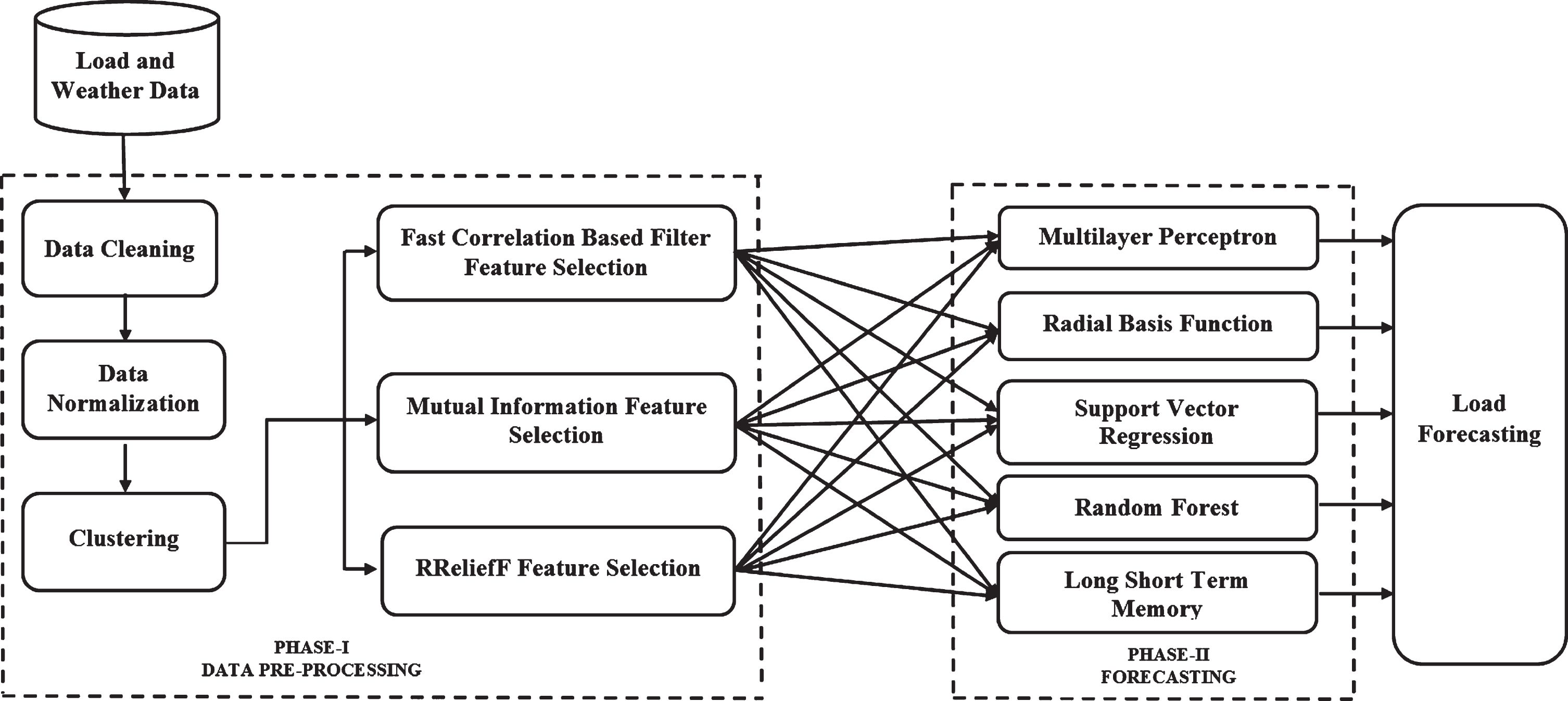
Short Term Load Forecasting with Filter Feature Selection.
The data preprocessing is an important task to be carried out before predictive analysis. As the prediction process depends on the historical data, the quality of the predictive analysis also depends on the input quality. While the historical data consists of incompleteness, it may lead to inaccurate predictions. In order to achieve an accurate prediction of the load, the historical input data should be preprocessed [35].
First, the hourly recorded electricity load and weather data are integrated and cleaned. Then, the date feature is extracted from the calendar features for an indexing purpose. After that, the min-max normalization is applied to make the dataset suitable for further processing. Let ‘D’ be the dataset, ‘X’ be the feature, ‘minx’ be the minimum of ‘X’, ‘maxx’ be the maximum of ‘X’, original interval be [minx, maxx] and the new interval be [nminx, nmaxx] . Any value ‘v’ from the original interval is mapped into the new value ‘newv’ in the normalized interval [0, 1] by the min-max normalization as follows,
The clustering groups similar samples and identifies the outliers. The feature selection may consider all samples or random samples for calculating feature importance. When all samples are considered, it may affect the computation process of the feature selection whereas the consideration of only the random samples may misguide the feature selection process in calculating the feature importance [8, 51]. In order to overcome these difficulties, the clustering can be utilized before the feature selection. So, in this paper, the k-means clustering was utilized to assist the feature selection in identifying the relevant features [20, 50]. First, similar sequences of load samples are grouped by using k-means clustering and removed the outliers. Then, the stratified samples are taken from each cluster by the filter feature selection for identifying the relevant features related to load [21, 49]. The pseudocode for the clustering-based filter feature selection is shown in Fig. 2. The following section discusses the step by step procedure for the clustering-based filter feature selection.
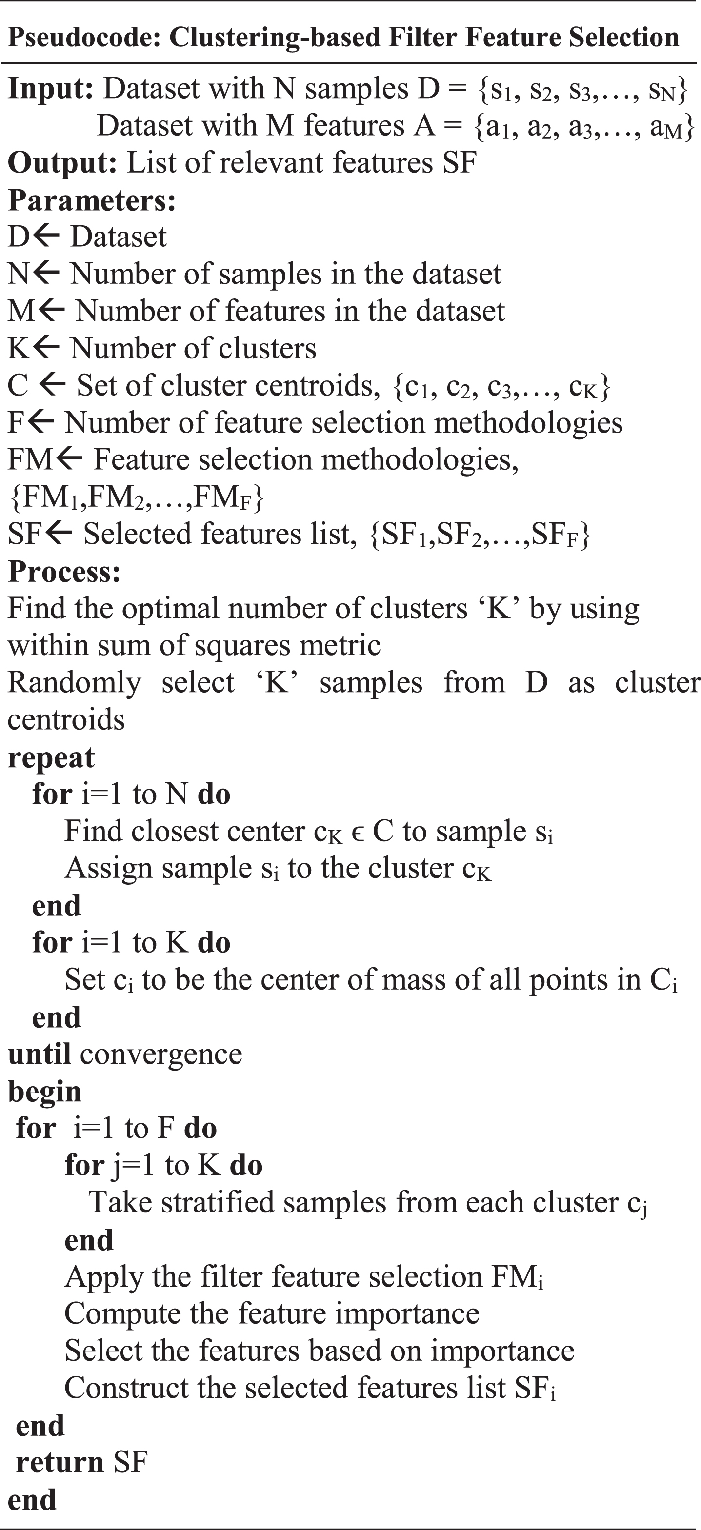
Pseudocode for Clustering-based Filter Feature Selection.
First, it finds the optimal number of clusters by using within sum of squares (WSS) metric as follows,
Consequently, it selects the final optimal number of clusters ‘k’ using the WSS value. Then, it selects ‘k’ samples from ‘D’ as the cluster centroids. After that, identify the similar samples for each cluster centroid from the dataset ‘D’ by using the Euclidean distance formula as follows,
The ‘n’ and ‘m’ represents two samples from the dataset and d(m,n) represents the distance between ‘m’ and ‘n’. Then, it forms the clusters by using similar samples belongs to each cluster centroids. After that, it updates the cluster centroids by calculating the mean sample (mc,nc) from the number of samples belongs to that cluster as follows,
Repeat the same process until there is no change in the cluster formation. Then, it takes the stratified samples from each cluster and finds the relevant features using filter feature selection. The list of features selected is utilized by the forecasting models for forecasting the future load demand.
The feature selection has a prominent role in reducing the complexity of the forecasting by providing reduced data in terms of relevant features. When the dataset has irrelevant features, it makes the model becomes complicated. So, identifying relevant features is an inevitable task that needs to be done to achieve an accurate prediction [32, 53]. It also helps to reduce the overfitting and curse of dimensionality problems during learning which in turn improves the accuracy of forecasting. Due to the rapid growth of load data in the power system and also the high correlation of load with other environmental factors, the feature selection becomes a crucial preprocessing task need to be done before forecasting the load.
Fast Correlation Based Filter: The FCBF is a type of filter feature selection that uses the symmetric uncertainty(SU) for measuring the relationship between features. It calculates the relationship between the feature-feature and feature-target. It also prunes the features that are redundant as they have a high correlation with other features. The useful features must have high relevance with the target, but it should not be redundant to any other relevant features. As the load has non-linear nature, the information theory-based correlation measure is utilized to find the relationship between features [29].
Let ‘S’ be the dataset with ‘n’ number of features f1, f2, f3,..., fn and the target feature ‘c’. First, set the predefined threshold value ‘δ’ for identifying the relevant features. Then, calculate the SU for each feature ‘fi’ with the target feature ‘c’. The SU is a valuable property to measure the relationship between two features. When the features have high correlation, the SU(fi, c) value is 1, otherwise it is 0. It is calculated as follows,
When the feature ‘fi’ is more correlated than the feature ‘fj’ with the target feature ‘c’, the information gain of ‘fi’ is higher than the information gain of ‘fj’, IG (fi|c) > IG (fj|c). Where H(fi) represents the entropy of the feature ‘fi’ and is defined as follows,
Mutual Information: The mutual information is a non-linear correlation-based feature selection that calculates the information shared by two or more features. The independent features do not give any information about other features. The dependency or the amount of information shared by one feature with other features is called an entropy [43]. Let ‘X’ and ‘Y’ are two features, then the mutual information between them is denoted as I(X;Y). The I(X;Y) is 0 when both ’X’ and ‘Y’ are independent. As the load data is continuous the mutual information of the feature ‘X’ with target ‘Y’ is calculated as follows,
RReliefF: The RReliefF supports the non-myopic discretization of numeric features. As the target feature is continuous in regression problems, the hit and misses cannot be utilized to estimate the feature weight. So, instead of hits and misses, it uses the kind of probability that denotes the predicted value of two instances that are different. The probability is modeled by using the relative distance of the predicted value between two instances. The RReliefF estimates the weight of each feature by taking random samples from the dataset and provides all features along with its weight. The features with the highest weight are considered as relevant features. The following section demonstrates the working of the RReliefF.
Let ‘x’ represents the vector of attribute values and ‘τ(x)‘ represents the predictor value. Initially, the RReliefF algorithm initializes the weight value for all features to 0. Then, it selects the sample ‘Ri‘randomly from the dataset. After that, it finds the k-nearest instances to ‘Ri‘ and calculates the weight for different predictions (NdC) [34].
Next, it calculates the weight for different predictions and attributes NdC &dA as follows,
Finally, it calculates the weight for each attribute as follows,
The vector ‘W’ has the final list of selected features [24].
The forecasting of the short term load demand is performed using LSTM and compared against MLP, RBF, SVR, and RF. As the real time load is the complex, uncertain, volatile, time series and non-linear, the statistical methods cannot handle it effectively and fail to provide accurate forecasting [28]. As the MLP [15], RBF [6], SVR [66] and RF [16] are suitable for processing the load with minimal overfitting and high accuracy, these models are elected as the competing models. Once the model is trained, it is utilized for forecasting the future load efficiently and more accurately.
Multilayer perceptron
The multilayer perceptron is an acyclic and directed feed-forward artificial neural network. It consists of many layers, such as one input layer, one or more hidden layers, and only one output layer [24]. In the multilayer perceptron, the number of neurons are organized in each layer. The neurons in different layers are connected by using weighted links. All the neurons except the neurons in the input layer use the non-linear activation function. The MLP model is suitable for regression problems and also it has an ability to handle the non-linear data with many features and number of inputs. Hence, it can easily differentiate the data that is not linearly separable and also the prediction with MLP is very fast. The structure of the MLP is shown in Fig. 3.
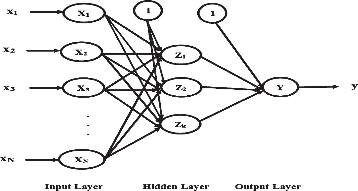
Structure of Multilayer Perceptron.
The inputs (x) provided at the input layer (X) are passed to the hidden layer (Z) and the outcome of the hidden layer is passed to the output layer (Y). At each hidden and output neurons, the sum of input with its connection weight provides the net activation of that neuron. The value of the activation function is determined by the transfer function, usually sigmoid function.
The radial basis function performs supervised learning and effectively handles the regression and time series prediction problems. It functions same as that of the feed-forward network, but it uses one hidden layer and Gaussian functions as an activation function in each hidden unit. The hidden layer acts as a tuned processor and each hidden unit in that layer acts as a pattern detector that detects the score for matching an input vector and its connection weight. The hidden layer consists of non-linear units which have separate activation function, center, parameter and width. It approximates the multivariate functions locally and captures effectively the uncertainty of the model using the Gaussian function [6, 46].
Support vector regression
The SVR is the stable model for handling the non-linear data. It has the regularization capability and can handle regression problems effectively by maintaining all the necessary characteristics related to the maximal margin as that of SVM. It does not suffer from the overfitting. It uses the non-linear mapping for mapping the input vector ‘X’ onto ‘m’ dimensional feature space [35, 66]. After that, the linear model, f(X,w), is developed as follows,
The complexity of SVR can be reduced by minimizing ∥w ∥ 2. The deviation outside the ɛ-intensive zone is measured by introducing slack variables, ξi, ξ*, in the training sample for minimizing ∥w ∥ 2. The minimized SVR model is expressed as follows,
The accuracy of SVR can be improved by setting carefully the ‘ɛ’ and the kernel parameters [33].
The random forest is utilized as the black box model due to its built-in ensembling capability. It handles regression problems with high robustness to the correlated features. It is the powerful stable algorithm appropriate for the regression problems which has an ability to reduce the overfitting of the model effectively [16]. When it is used for a regression problems, it is called random forest regressor. It is the supervised and tree based machine learning algorithm of versatile nature. It builds the forest by constructing multiple ensembles of decision trees. The random forest searches the best features among its random subset of features. The function of the random forest depends on bagging and random feature selection [43]. The bootstrap samples are taken by sampling with replacement from training data and the features are selected randomly for constructing the bag. If ‘p’ number of features in the dataset, then √p number of features are selected for building each tree. Finally, the outcome of all the ensemble decision trees are merged for improving the generalization capability of the model [2].
Long short term memory
The long short term memory is a variant of RNN, which is developed for solving the vanishing gradient and exploding gradient problems of simple RNN. The RNN takes a vector of the input sequence, models in each hidden node and maintains the state information that can be utilized as one of the input for the next modeling at the same node. It produces the output by considering the past input and past computations at each time [58]. It is accomplished by embedding the previous event information at the hidden state variables. As the RNN has a limited memory, it has the ability to remember short sequences. The LSTM overcomes this difficulty by keeping the information for a long period using gates in each cell. Instead of neurons, the LSTM network uses memory that replaces the short term memory of RNN. So, the LSTM can preserve information for a long sequence [9]. Thus, it enables an adequate understanding of the sequence dependence exists in the time series load data. The architecture of the LSTM cell is given in Fig. 4. The gates in the LSTM cell regulates the flow of information and decides upon the relevant information to be kept and the irrelevant information to be forgotten. The LSTM cell uses three types of gates, namely forget gate, input gate, and output gate. The forget gate finds the information which should be thrown away from the cell state. The input gate decides the new information from the input to be added to the cell state for updating the memory from the old cell state ‘Ct - 1’ to the current state ‘Ct . ’. The output gate decides what information, Ot, from the cell state can be included in the output.
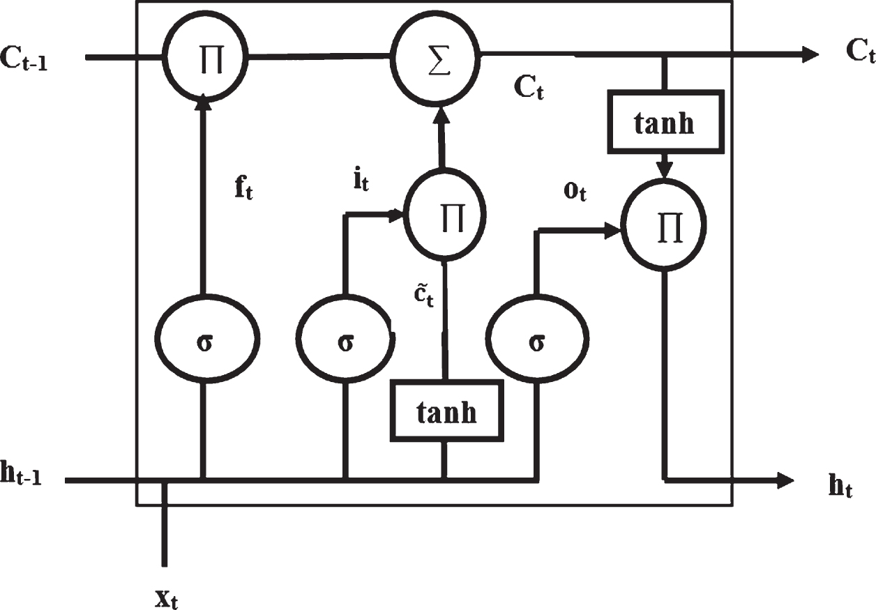
Architecture of Long Short Term Memory cell.
Let the input sequence be {x1, x2, x3, ... , xn}, the input at time ‘t’ be ‘xt’, the previous hidden state at time ‘t-1’ be ‘ht - 1’ and the the new hidden state at time ‘t’ be ‘ht‘. The ‘Ct - 1’, ‘Ct’ and ‘
where Wf, Wi, Wc and Wo represents the weight matrix of forget gate, input gate during sigmoid function, input gate during tanh function and output gate respectively. The bf, bi, bc and bo represents the bias weight matrix of forget gate, input gate during sigmoid function, input gate during tanh function and output gate respectively. The performance of the LSTM can be improved by increasing the depth of the model [27].
In the present paper, the historical load and weather data of two European countries, Switzerland (DST-I) and France (DST-II), were used to show the generality of the proposed model. The load and weather data recorded at every hour from 1st January 2008 to 31st December 2012 is considered for the experiment. The load dataset consists of 24 hrs recording of load values along with day, month, year and minute values. The weather dataset consists of 20 meteorological features with four calendar features day, month, year and minute. The load has high correlation with weather values. So, the load and weather values are merged to form the dataset that is suitable for forecasting. The redundant calendar features from the weather data are removed manually. Now, the dataset consists of 25 features and 43848 instances. The new feature named ‘date’ is extracted from the ‘day’, ‘month’, ‘year’ and ‘minute’ features for an index purpose. Finally, the dataset with 22 features and 43848 instances are utilized for forecasting the short term load.
The sample of load demand from two datasets, DST-I and DST-II, are plotted in Fig. 5 and Fig. 6 respectively.
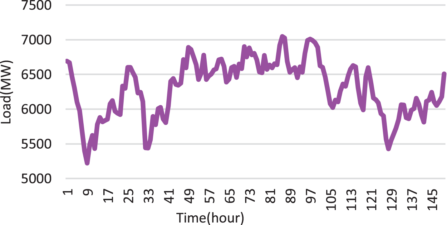
Sample of load demand from DST-I.
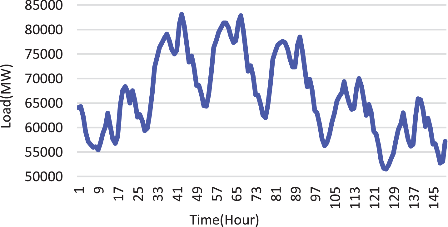
Sample of load demand from DST-II.
The datasets with different characteristics such as load demand range and load demand trend are considered to show the generality of the proposed model. The minimum, maximum and mean load demand of the DST-I are 229 MW, 8694 MW and 5633 MW respectively. On the otherhand, the minimum, maximum and mean load demand of the DST-II are 30826 MW, 102098 MW and 56051 MW respectively. The load demand trend has more fluctuations in DST-I, whereas the DST-II has a smooth load trend compared to DST-I. The dataset is partitioned into training dataset, validation dataset and testing dataset. The load data from 1st January 2008 to 31st December 2010 is utilized as training data, the load data from 1st January 2011 to 31st December 2011 is utilized as validation data and the load data from 1st January 2012 to 31st December 2012 is used as the testing data.
The list of features of the dataset are f1-Date, f2-Load, f3-Temperature, f4- Relative Humidity, f5- Pressure, f6- Total precipitation amount (high resolution, limited time range), f7- Total precipitation amount (low resolution), f8- Snowfall amount (high resolution, limited time range), f9- Snowfall amount (low resolution), f10- Total cloud cover, f11- Low cloud cover, f12- Medium cloud cover, f13- High cloud cover, f14- Sunshine Duration, f15- Shortwave Radiation, f16- Wind Speed [10 m above gnd], f17- Wind Direction [10 m above gnd], f18- Wind Speed [80 m above gnd], f19- Wind Direction [80 m above gnd], f20- Wind Speed [900 m above gnd], f21- Wind Direction [900 m above gnd] and f22- Wind Gust. The following section discusses the experimental results obtained with DST-I.
To improve the forecasting performance the clustering-based filter feature selection such as FCBF, MI, and RReliefF are applied individually on the dataset and the relevant features are obtained. After performing the feature selection on DST-I, 13 features are selected as the relevant features related to load feature. The features selected by the feature selection for the DST-I are listed in Table 1.
Selected Features from DST-I
The LSTM model is trained by using the training dataset. The load and weather data at the previous time step is given as input and the load data at the next timestep is forecasted. The LSTM network is configured by setting the number of inputs as 13 for DST-I, the number of inputs as 12 for DST-II, the number of output as 1, number of hidden layers are tested from 1 to 10 and selected 2 as the optimal, the number of units in the hidden layers are tested from 10 to 100 and selected 20 as optimal, the number of epochs tested from 100 to 500 and selected 150 as optimal, the optimizer as Adam and the loss function as mean absolute error.
Consequently, the performance of the models are enhanced by tuning its parameters using the validation dataset. Generally the traditional time series forecasting methods produce less accurate results when the time interval between the training time and forecasting time increases. In this paper, to overcome this limitation, the time series cross-validation on a rolling basis is utilized as the validation technique. The forecasting of the short term load is performed by using LSTM and compared against MLP, RBF, SVR, and RF with all features and selected features. The comparison of the actual and forecast load of DST-I is plotted in Fig. 7. It shows that the forecasting model with selected features provided by the feature selection produces better results compared to the models with all features. The LSTM with the RReliefF feature selection surpassed other models. The LSTM is more suitable for time series data. It extracts the features from the input and keeps the sequence dependency for a longer period. The selected features provided by the feature selection also help the LSTM to reduce the complexity of feature extraction from the number of features. Generally, the performance of the forecasting model is evaluated in many ways. In this paper, the MAPE, MAE, MSE, and RMSE are utilized as the evaluation measures and are defined as follows,
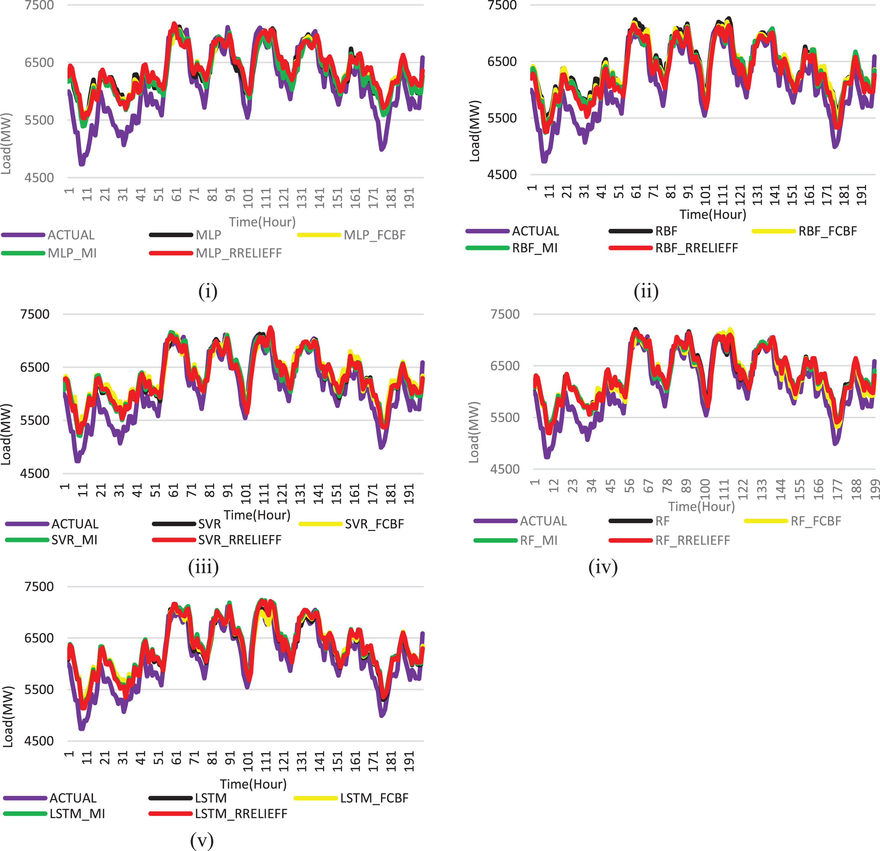
Forecasting Results of DST-I. (i) Comparison of actual and forecast load using MLP. (ii) Comparison of actual and forecast load using RBF. (iii) Comparison of actual and forecast load using SVR. (iv) Comparison of actual and forecast load using RF. (v) Comparison of actual and forecast load using LSTM.
Comparison of Forecasting Results of DST-I in terms of MAPE, MAE, MSE and RMSE
The forecasting performance of the LSTM with RReliefF is also tested using DST-II. The following section discusses the experimental results obtained from DST-II. The dataset consists of 22 features and 43848 instances as DST-I. The relevant features which contribute to improve the forecasting performance of DST-II are identified by using filter feature selection such as FCBF, MI, and RReliefF. The merit score of the features flatten after 12 features. So, the topmost 12 features are identified as the important features related to the load. The list of features selected by the FCBF, MI, and RReliefF feature selection are shown in Table 3.
Selected Features from DST-II
The load and weather data at the pevious timestep is given as input to the LSTM model and the load at the next timestep is forecasted. The forecasting of the load demand of DST-II for the year 2012 is performed by using LSTM and compared against MLP, RBF, SVR, and RF with all features and selected features. Figure 8 shows the comparison of actual and forecast load for DST-II. The DST-II has a smooth load trend compared to DST-I. So, the LSTM with RReliefF learns effectively the sequence dependency exists in the load data. As a result, it produced more accurate forecast compared to DST-I. It proves that the LSTM with RReliefF works well for DST-II also.
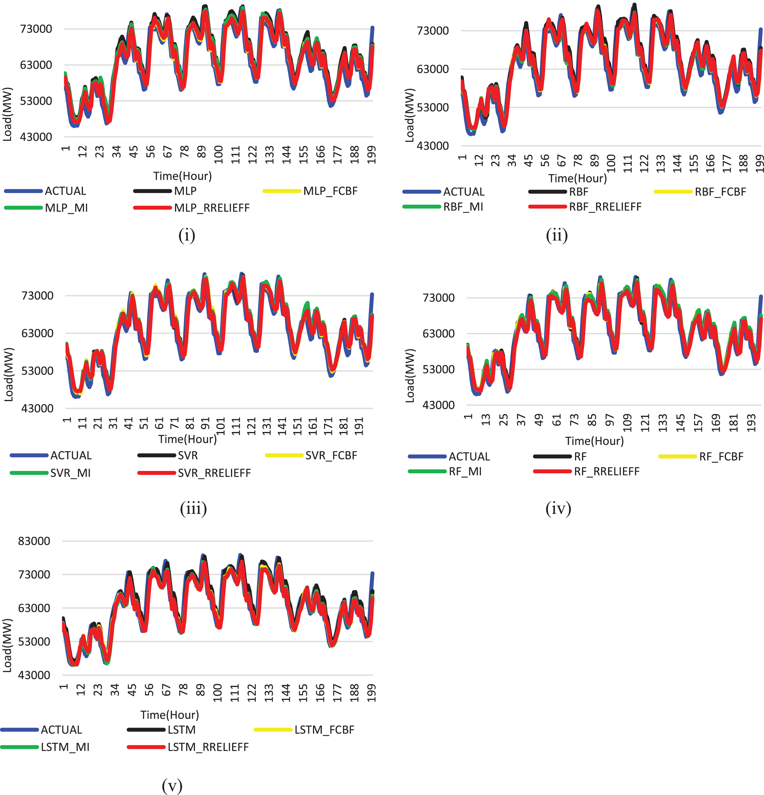
Forecasting Results of DST-II. (i) Comparison of actual and forecast load using MLP. (ii) Comparison of actual and forecast load using RBF. (iii) Comparison of actual and forecast load using SVR. (iv) Comparison of actual and forecast load using RF. (v) Comparison of actual and forecast load using LSTM.
Table 4 shows the comparison of forecasting results of DST-II in terms of MAPE, MAE, MSE, and RMSE. It shows that the forecasting models with feature selection achieved better performance compared to the model without feature selection. The LSTM with RReliefF outperformed other models due to the two levels of the feature extraction. The first level extraction by the external feature selection and second level extraction by its internal feature extraction capability. So, it utilizes all the relevant features that contribute to forecast the future load and provides better results.
Comparison of Forecasting Results of DST-II in terms of MAPE, MAE, MSE and RMSE
The time complexity of the short term load forecasting using LSTM with RReliefF is O(n/2.a+w). The nearest instances are found for calculating the importance of feature require O(n/2.a) steps for ‘a’ features and ‘n’ instances. The computational complexity to update each weight in LSTM per time step is O(1). Hence, the overall complexity of LSTM per timestep is O(w), where ‘w’ represents the number of weight. The analysis of the forecasting errors shown in Table 2 and Table 4 confirms that the necessity of LSTM with RReliefF for producing an accurate result. In addition to that the training time of the LSTM with RReliefF is also compared against MLP, RBF, SVR, and RF. For DST-I, the training time of MLP, RBF, SVR, RF, LSTM and LSTM with RReliefF are 194 s, 157 s, 128 s, 106 s, 31 s and 15 s respectively. For DST-II, the training time of MLP, RBF, SVR, RF, LSTM and LSTM with RReliefF are 190 s, 162 s, 104 s, 85 s, 25 s and 12 s respectively. Due to the removal of outliers, the reduction of dimension of data, and the effective handling of non-linear temporal dependency, the complexity and the training time of the LSTM with RReliefF is drastically reduced compared to others.
The superiority of the LSTM with RReliefF is verified in terms of the performance measures such as MAPE, MAE, MSE, and RMSE. In addition to that, two statistical tests also conducted to demonstrate the improvement of the forecasting performance of LSTM with RReliefF. In the present paper, based on the research recommendations provided by [13] and [31], the Wilcoxon signed-rank test (pairwise comparison test) and the Friedman test (multiple comparisons test) are conducted to verify the significance of the LSTM with RReliefF model.
The Wilcoxon signed-rank test is the famous nonparametric test conducted between two sets of data with the same size. It is used to perform the pairwise significant test between two models. It is based on difference scores as a sign test. However, in addition to analyze the signs of the differences, it also takes into account the magnitude of the observed differences. It assumes the null hypothesis (H0) as the medians of the differences between the two group samples are equal. The ith forecasting error (ei) is calculated from the ith forecast values of the two models and are used to measure the statistic value (Wstatistic) as follows,
The Friedman test is also a nonparametric statistical test. It determines the significant differences between the forecasting errors produced by two or more models. It assumes the null hypothesis as the means of the forecasting errors of two or more models are same [18, 69]. The statistic ‘F’ of the Friedman test is measured as follows,
If the statistic value of ‘F’ is larger than the Friedman critical value (which is obtained from the Friedman critical value table) and the p-value is less than ‘α’, then the null hypothesis is rejected. The results of the Wilcoxon signed-rank test and the Friedman test for DST-I and DST-II are shown in Table 5 and Table 6 respectively.
Results of Wilcoxon signed-rank test and Friedman test obtained from DST-I
bIndicates that the LSTM with RReliefF significantly surpasses other compared models; *Represents that the test indicates not to accept the null hypothesis under α= 0.02; **Represents that the test indicates not to accept the null hypothesis under α= 0.05.
Results of Wilcoxon signed-rank test and Friedman test obtained from DST-II
bIndicates that the LSTM with RReliefF significantly surpasses the other compared models; *Represents that the test indicates not to accept the null hypothesis under α= 0.02; **Represents that the test indicates not to accept the null hypothesis under α= 0.05.
For DST-I, the Wilcoxon signed-rank test is conducted between each pair of models by setting the significance level, α= 0.02 and α= 0.05. In both cases, the Wilcoxon signed-rank test produces ‘Wstatistics’ value less than the critical value ‘W’ and also the p-value is less than ‘α’. So, the null hypothesis is rejected. The multiple comparison Friedman test is conducted by setting the α= 0.05. The null hypothesis is rejected since the p-value is less than ‘α’ and the Friedman statistic value ‘F’ is larger than the Friedman critical value. The Wilcoxon signed-rank test and Friedman test show that the LSTM with RReliefF model is superior compared to other models.
The superiority of the LSTM with RReliefF is also tested with DST-II.The Wilcoxon signed-rank test and Friedman test are applied by setting the significance level, α= 0.02 and α= 0.05. The Friedman test is also conducted by setting the α= 0.05. In both test, the null hypothesis is rejected. The significant test results showed in Table 5 and Table 6 represents the feature selection adds significant contribution in improving the performance of the forecasting. From both case studies using DST-I and DST-II, the performance measures such as MAPE, MAE, MSE and RMSE and Statistical tests such as Wilcoxon signed-rank test and Friedman test proves that the LSTM with RReliefF significantly outperformed other models.
The electricity load forecasting is becoming one of the critical issue to solve the energy crisis problems. This has become an important research area of global concern. The short term load forecasting has a crucial role in the power system planning, scheduling, operation, dispatching and maintenance. In this paper, the clustering-based filter feature selection was introduced to remove the outliers, reduce the curse of dimensionality, reduce the overfitting issues with short term load forecasting. In this paper, the performance of the forecasting was improved by removing the outliers using clustering, reducing the curse of dimensionality by removing the irrelevant features using the filter feature selection such as FCBF, MI, and RReliefF and reducing the overfitting using the deep recurrent neural network based LSTM. It considers calendar, weather and load features for forecasting the short term load. The performance of the forecasting models was evaluated in terms of MAPE, MAE, MSE, and RMSE. The LSTM with RReliefF model outperformed others by producing least error. Hence, the generality of the LSTM with RReliefF was proved using the hourly recorded historical load demand and weather data of two European countries. The computational time was also reduced drastically by effectively removing the irrelevant features and outliers. The significance of the LSTM with RReliefF model was also verified by conducting the Wilcoxon signed-rank test and the Friedman test. The result shows that the short term load forecasting with filter feature selection especially, the LSTM with RReliefF surpassed other models. In the future, hybrid feature selection can also be incorporated with machine learning and deep learning to improve the forecasting performance.