A nonparallel support vector machine with pinball loss for pattern classification

Abstract

In this paper, we propose a nonparallel support vector machine with pinball loss (Pin-NPSVM) that deals with the noise sensitivity and resampling instability of NPSVM. More specifically, we redefine a pinball loss funtion and build a pair of quantile hyper-planes. Each quantile hyper-plane is constructed by using the new pinball loss instead of ɛ-insensitive loss, which makes the new classification model be insensitive to noise samples, especially for feature noise samples around the decision boundary. Moreover, instead of hinge loss, Pin-NPSVM also builds a pair of decision boundaries based on traditional pinball loss, which further improves the anti-nosie ability of the classification model. In a word, Pin-NPSVM not only inherits the characteristics of the nonparallel optimal hyper-planes, but also has a consistent model with Pin-SVM, which can process noise data well. Finally, numerical experimental results show that the Pin-NPSVM has more obvious advantages than other models in classification performance, especially for noise datasets.

Keywords

Pattern classification nonparallel support vector machine pinball loss anti-noise

1 Introduction

Classification is one of the main problems in the field of data mining. There are varieties of algorithms [1 –6] being used in classification technique. By comparsion, the support vector machine (SVM) [7] has advantages for solving the classification problem with small-scale data. Firstly, SVM adopts the principle of structural risk minimization and has good generalization performance. Secondly, SVM obtains an optimal classification hyper-plane by solving a quadratic programming problem (QPP) [8], which makes sure to find the global optimal solution. Thirdly, SVM uses the kernel function to transform nonlinear problem into linear problem, avoiding the dimension disaster and complexity of calculation. At present, SVM has been successfully applied in the fields of pattern classification and regression analysis [9 –11]. Even so, there are spaces for improvement in SVM. On the one hand, SVM needs a lot of time to solve a large QPP. On the other hand, SVM is sensitive to noise, especially for feature noise around the decision boundary.

In order to improve the performance of SVM, many improved algorithms have been proposed. Such as, least squares support vector machine (LSSVM) [12], proximal SVM via generalized eigenvalues (GEPSVM) [13], and support vector data description (SVDD) [14]. The most typical one is twin support vector machine (TSVM) [15]. TSVM proposed by Jayadeva is derived from GEPSVM, and is similar to SVM in formula. The essence of TSVM is to determine two nonparallel hyper-planes by solving a pair of small QPPs. The nonparallel structure of TSVM makes itself more adaptive and robust. For example, TSVM is very suitable for the classification of cross datasets. In addition, TSVM replaces a complete QPP with two smaller QPPs, making its own computation four times faster than SVM. Therefore, in recent years, TSVM has been widely concerned and a series of improved TSVM algorithms have been proposed, such as v-TSVM [16], least squares TSVM (LS-TSVM) [17], twin bound SVM (TBSVM) [18] and nonparallel SVM (NPSVM) [19]. The validity and generalization of these models have been improved.

Furthermore, in order to suppress the adverse influence of noise samples for classification performance, various methods [17 –20] have been proposed by scholars. For example, Vapnik et al. [20] proposed a method to discover information patterns from data, which can not only reduce the number of samples, but also remove noise samples. Herbrich et al. [21] proposed adapative margin SVM (AM-SVM), which uses the adapative margin to redefine the minimization problem in original SVM. This model can improve the robustness against outliers. Zhang et al. [22] and Qi et al. [23] respectively proposed rough margin SVM (RMSVM) and rough TSVM (R-TSVM). Both of these models realized the anti-noise ability by using rough set theory. Subsequently, Huang et al. [24] constructed a novel SVM model (Pin-SVM) based on pinball loss. It was first one to introduce the pinball loss into SVM. Theory and practice show that Pin-SVM can effectively supress noise. However, Pin-SVM cannot adapt to the classification of cross dataset.

As we know, nonparallel SVM-based classifiers do an excellent job of handling cross datasets. NPSVM is a representative achievement in the nonparallel classifiers. NPSVM seeks a pair of nonparallel hyper-planes by using the ɛ-insensitive loss and hinge loss functions. Unlike TSVM, NPSVM has the whole sparseness and does not have to calculate the inverse of matrices. But, one can see that only a part of training samples contribute to the hyper-planes. If there are a few noise samples, the hyper-planes will be changed, resulting in poor classification performance. This shows NPSVM is very sensitive to noise, which is consistent with that of standard SVM.

Hence, in this paper, inspired by Pin-SVM, the concept of pinball loss is applied to NPSVM model, and a novel NPSVM model (Pin-NPSVM) based on pinball loss is built. The proposed model not only improve the anti-noise ability of NPSVM, but also improve the generalization performance of Pin-SVM. The main characteristics of Pin-NPSVM are as follows:

The construction idea of Pin-NPSVM is similar to TSVM. A big QPP in Pin-SVM is decomposed into two small related QPPs. And two nonparallel hyper-planes are built in Pin-NPSVM, such that each hyper-plane is proximal to data samples of one class and as far as possible from data samples of the other class.

The structure of Pin-NPSVM is similar to that of NPSVM, which is suitable for the classification of cross datasets. Therefore, Pin-NPSVM proposed in this paper has better adaptability and generalization than Pin-SVM.

Different from NPSVM, the pinball loss is used in Pin-NPSVM, rather than using ɛ-insensitivity loss and hinge loss, making Pin-NPSVM is insensitive to noise samples.

Compared with TSVM, Pin-NPSVM has the incomparable merits that the inverse of the matrices does not have to be computed and the kernel trick can be applied directly. Comparing to SVM, TSVM, NPSVM and Pin-SVM, the preliminary numerical experiments show that our Pin-NPSVM has good anti-noise ability and gains better generalization ability and adaptability.

The remainder of this paper is organized as follows. In Section 2, a brief review about NPSVM is given. Our Pin-NPSVM is formulated in Section 3. In Section 4, numerical experiments on several datasets are given in order to verify the validity and applicability of the proposed model. In the same section, we provide comparisons with SVM and other state of the art algorithms. In Section 5, we draw some conclusions and give directions for future work.

2 Brief introduction to NPSVM

Consider the binary classification problem with the training set $X = [(X^{+})^{T} (X^{-})^{T}]^{T},$ (1) where $X^{+} = [x_{1}^{+} x_{2}^{+} . . . x_{l^{+}}^{+}]^{T}$ represents the positive samples and l⁺ is the number of positive samples, $X^{-} = [x_{1}^{-} x_{2}^{-} . . . x_{m^{-}}^{-}]^{T}$ represents the negative samples and l^- is the number of negative samples.

For the linear case, NPSVM aims to construct a pair of nonparallel hyper-planes $\begin{matrix} f_{1} (x) = (w^{+})^{T} x + b^{+} = 0, \\ f_{2} (x) = (w^{-})^{T} x + b^{-} = 0 \end{matrix}$ (2) by optimizing two QPPs $\begin{matrix} min_{w^{+}, b^{+}} \frac{1}{2} | | w^{+} | |^{2} + c_{1} \sum_{i = 1}^{l^{+}} (η_{i} + η_{i}^{*}) + c_{2} \sum_{j = 1}^{l^{-}} ξ_{j} \\ s . t . (w^{+})^{T} x_{i}^{+} + b^{+} \leq ɛ + η_{i}, \\ - (w^{+})^{T} x_{i}^{+} - b^{+} \leq ɛ + η_{i}^{*}, \\ (w^{+})^{T} x_{j}^{-} + b^{+} \leq - 1 + ξ_{j}, \\ η_{i}, η_{i}^{*} \geq 0, ξ_{j} \geq 0, \\ i = 1, 2, . . ., l^{+}, j = 1, 2, . . ., l^{-}, \end{matrix}$ (3) $\begin{matrix} min_{w^{-}, b^{-}} \frac{1}{2} | | w^{-} | |^{2} + c_{3} \sum_{i = 1}^{l^{-}} (η_{i} + η_{i}^{*}) + c_{4} \sum_{j = 1}^{l^{+}} ξ_{j} \\ s . t . (w^{-})^{T} x_{i}^{-} + b^{-} \leq ɛ + η_{i}, \\ - (w^{-})^{T} x_{i}^{-} - b^{-} \leq ɛ + η_{i}^{*}, \\ (w^{-})^{T} x_{j}^{+} + b^{-} \geq 1 - ξ_{j}, \\ η_{i}, η_{i}^{*} \geq 0, ξ_{j} \geq 0, \\ i = 1, 2, . . ., l^{-}, j = 1, 2, . . ., l^{+}, \end{matrix}$ (4) where, ξ_j, η_i and $η_{i}^{*}$ are the slack variables, c_i (i = 1, 2, 3, 4) >0 are penalty parameters, and ɛ > 0 is an adjustable parameter that can better adjust the classification performance of the model. For the nonlinear case, the kernel trick can be applied directly.

3 Nonparallel support vector machine based on pinball loss

3.1 Pinball loss

Considering a binary classification problem, the positive class samples set is $X^{+} = [x_{1}^{+}, x_{2}^{+}, . . .,$ $x_{l^{+}}^{+}]^{T}$ , and the negative class samples set is $X^{-} = [x_{1}^{-}, x_{2}^{-}, . . ., x_{l^{-}}^{-}]^{T}$ . Pin-SVM was the first one to introduce the pinball loss into SVM, which improves the anti-noise ability. For Pin-SVM, by optimizing the pinball loss (5), two supporting hyper-planes $f_{S}^{+} : w^{T} x + b = + 1$ and $f_{S}^{-} : w^{T} x + b = - 1$ can be built. $\begin{matrix} y_{i} (w^{T} x_{i} + b) \geq 1 - ξ_{i}, \\ y_{i} (w^{T} x_{i} + b) \leq 1 + \frac{1}{τ} ξ_{i}, \end{matrix}$ (5) where τ is an adjustable parameter, the position of $f_{S}^{+}$ and $f_{S}^{-}$ is changed by adjusting the value of τ, which makes Pin-SVM is insensitive to noise, especially for feature noise around the supporting hyper-planes.

The concept of Pin-NPSVM is similar to that of Pin-SVM: the pinball loss is used. Differently, Pin-NPSVM searches for a pair of nonparallel quantile classification hyper-planes and two quantile boundaries. For quantile classification hyper-planes which are the same as (2), they are required to locate in the middle of positive and negative samples. In order to appropriately apply the idea of pinball loss into the Pin-NPSVM model, the pinball loss is redefined as the following. It is different from traditional pinball loss (5), since Pin-NPSVM builds the quantile classification hyper-planes $f_{h}^{\pm} : (w^{\pm})^{T} x + b^{\pm} = 0$ rather than w ^T x + b = ±1 of Pin-SVM. $\begin{matrix} (w^{+})^{T} x_{i}^{+} + b^{+} \leq 0 + \frac{1}{τ} η_{i}, \\ (w^{+})^{T} x_{i}^{+} + b^{+} \geq 0 - η_{i}^{*} . \end{matrix}$ (6) $\begin{matrix} (w^{-})^{T} x_{i}^{-} + b^{-} \geq 0 - η_{i}, \\ (w^{-})^{T} x_{i}^{-} + b^{-} \leq 0 + \frac{1}{τ} η_{i}^{*} . \end{matrix}$ (7)

Moreover, because the quantile classification hyper-planes only need to be in the middle of each class samples. and their positions do not need to be adjustable, the adjustable parameter τ in the (6) and (7) does not be changed. In this paper, let τ be equal to 1. Therefore, the pinball loss is reformulated as the following. $\begin{matrix} (w^{+})^{T} x_{i}^{+} + b^{+} \leq η_{i}, \\ (w^{+})^{T} x_{i}^{+} + b^{+} \geq - η_{i}^{*} . \end{matrix}$ (8) $\begin{matrix} (w^{-})^{T} x_{i}^{-} + b^{-} \geq - η_{i}, \\ (w^{-})^{T} x_{i}^{-} + b^{-} \leq η_{i}^{*} . \end{matrix}$ (9)

Because all samples contribute to the quantile hyper-planes, the prior structure information of samples is considered, which improves the robustness of model. For the boundaries $f_{b}^{+} : (w^{+})^{T} x + b^{+} = - 1$ and $f_{b}^{-} : (w^{-})^{T} x + b^{-} = + 1$ , the pinball loss is defined as the following, and the descriptions are similar to that of (5). $\begin{matrix} (w^{+})^{T} x_{j}^{-} + b^{+} \leq - 1 + ξ_{j}, \\ (w^{+})^{T} x_{j}^{-} + b^{+} \geq - 1 - \frac{1}{τ} ξ_{j}, \end{matrix}$ (10) $\begin{matrix} (w^{-})^{T} x_{j}^{+} + b^{-} \geq 1 - ξ_{j}, \\ (w^{-})^{T} x_{j}^{+} + b^{-} \leq 1 + \frac{1}{τ} ξ_{j}, \end{matrix}$ (11)

3.2 Linear Pin-NPSVM

Inspired by Pin-SVM and NPSVM, the standard pinball loss and redefined pinball loss are introduced to obtain the following Pin-NPSVM, $\begin{matrix} min_{w^{+}, b^{+}} \frac{1}{2} | | w^{+} | |^{2} + c_{1} \sum_{i = 1}^{l^{+}} (η_{i} + η_{i}^{*}) + c_{2} \sum_{j = 1}^{l^{-}} ξ_{j} \\ s . t . (w^{+})^{T} x_{i}^{+} + b^{+} \leq 0 + η_{i}, \\ (w^{+})^{T} x_{i}^{+} + b^{+} \geq 0 - η_{i}^{*}, \\ (w^{+})^{T} x_{j}^{-} + b^{+} \leq - 1 + ξ_{j}, \\ (w^{+})^{T} x_{j}^{-} + b^{+} \geq - 1 - \frac{1}{τ} ξ_{j}, \\ η_{i}, η_{i}^{*} \geq 0, i = 1, 2, . . ., l^{+}, j = 1, 2, . . ., l^{-}, \end{matrix}$ (12) $\begin{matrix} min_{w^{-}, b^{-}} \frac{1}{2} | | w^{-} | |^{2} + c_{3} \sum_{i = 1}^{l^{-}} (η_{i} + η_{i}^{*}) + c_{4} \sum_{j = 1}^{l^{+}} ξ_{j} \\ s . t . (w^{-})^{T} x_{i}^{-} + b^{-} \geq 0 - η_{i}, \\ (w^{-})^{T} x_{i}^{-} + b^{-} \leq 0 + η_{i}^{*}, \\ (w^{-})^{T} x_{j}^{+} + b^{-} \geq 1 - ξ_{j}, \\ (w^{-})^{T} x_{j}^{+} + b^{-} \leq 1 + \frac{1}{τ} ξ_{j}, \\ η_{i}, η_{i}^{*} \geq 0, i = 1, 2, . . ., l^{-}, j = 1, 2, . . ., l^{+}, \end{matrix}$ (13) where c_i (i = 1, 2, 3, 4) >0 are preset parameters, which are used to keep the balance of each term in (12) and (13). $η_{i}^{(*)}$ and ξ_j are positive slack variables. And τ is an adjustable parameter.

For (12), $x_{i}^{+}$ represents target class sample, and $x_{j}^{-}$ is background sample. With this formulation, we build a classification hyper-plane $f_{h}^{+}$ and a boundary $f_{b}^{+}$ . Now, we discuss the primal problem (12) geometrically. The first term of objective function aims to maximize the margin between $f_{h}^{+}$ and $f_{b}^{+}$ , which makes the different classes samples are separable. The first and the second constraints are the redefined pinball loss, the pinball loss is optimized to construct the classification hyper-plane $f_{h}^{+}$ , which is located in the middle of the target class samples. All samples contribute to the hyper-place, which makes the Pin-NPSVM can explore the prior structure information of the target class samples and improve the generalization performance of the model. Meanwhile, the introduction of pinball loss makes the classification hyper-plane is insensitive to noise. The third and the fourth constraints are the standard pinball loss, which are used to build a boundary hyper-plane $f_{b}^{+}$ . By adjusting the value of τ, the boundary $f_{b}^{+}$ is also insensitive to noise. The errors $η_{i} + η_{i}^{*}$ and ξ_j are measured by the pinball loss. In terms of attributes and conclusions, the optimization problem (13) is similar to (12). Therefore, it is not necessary to analyze (13) again.

To derive the dual problem, we introduce the following Lagrange function: $\begin{matrix} L = \frac{1}{2} | | w^{+} | |^{2} + c_{1} \sum_{i = 1}^{l^{+}} (η_{i} + η_{i}^{*}) + c_{2} \sum_{j = 1}^{l^{-}} ξ_{j} \\ + \sum_{i = 1}^{l^{+}} α_{i} ((w^{+})^{T} x_{i}^{+} + b^{+} - η_{i}) - \sum_{i = 1}^{l^{+}} γ_{i} η_{i} \\ - \sum_{i = 1}^{l^{+}} α_{i}^{*} ((w^{+})^{T} x_{i}^{+} + b^{+} + η_{i}^{*}) - \sum_{i = 1}^{l^{+}} γ_{i}^{*} η_{i}^{*} \\ + \sum_{j = 1}^{l^{-}} β_{j} ((w^{+})^{T} x_{j}^{-} + b^{+} + 1 - ξ_{j}) \\ - \sum_{j = 1}^{l^{-}} θ_{j} ((w^{+})^{T} x_{j}^{-} + b^{+} + 1 + \frac{1}{τ} ξ_{j}) \end{matrix}$ (14) where both $α_{i}^{(*)}, β_{j}, θ_{j}$ and $γ_{i}^{(*)}$ are Lagrange multipliers. According to the Karush-Kuhn-Tucker conditions, we can get $\frac{\partial L}{\partial w^{+}} = w^{+} - \sum_{i = 1}^{l^{+}} (α_{i}^{*} - α_{i}) x_{i}^{+} - \sum_{j = 1}^{l^{-}} (θ_{j} - β_{j}) x_{j}^{-},$ (15) $\frac{\partial L}{\partial b^{+}} = - \sum_{i = 1}^{l^{+}} (α_{i}^{*} - α_{i}) + \sum_{j = 1}^{l^{-}} (β_{j} - θ_{j}) = 0,$ (16) $\frac{\partial L}{\partial η_{i}} = c_{1} - α_{i} - γ_{i} = 0,$ (17) $\frac{\partial L}{\partial η_{i}^{*}} = c_{1} - α_{i}^{*} - γ_{i}^{*} = 0,$ (18) $\frac{\partial L}{\partial ξ_{j}} = c_{2} - β_{j} - \frac{1}{τ} θ_{j} = 0 .$ (19)

Let $μ_{i}^{+} = (α_{i}^{*} - α_{i}), ϑ_{j}^{-} = β_{j} - θ_{j}$ , the formulations (15) and (16) can be simplified to $w^{+} = \sum_{i = 1}^{l^{+}} μ_{i}^{+} x_{i}^{+} - \sum_{j = 1}^{l^{-}} ϑ_{j}^{-} x_{j}^{-},$ (20) $- (e^{+})^{T} μ^{+} + (e^{-})^{T} ϑ^{-} = 0,$ (21) where e ⁺ = (1, . . . , 1) ^T ∈ R^{l
⁺}, e ^- = (1, . . . , 1) ^T ∈ R^{l
^-}.

According to (14–21), the Lagrange function (14) can be simplified. And the dual optimization problem of (12) is obtained as follows: $\begin{matrix} min_{μ^{+}, ϑ^{-}} \frac{1}{2} (μ^{+})^{T} X^{+} (X^{+})^{T} μ^{+} - (μ^{+})^{T} X^{+} (X^{-})^{T} ϑ^{-} \\ + \frac{1}{2} (ϑ^{-})^{T} X^{-} (X^{-})^{T} ϑ^{-} - (e^{-})^{T} ϑ^{-} \\ s . t . - (e^{+})^{T} μ^{+} + (e^{-})^{T} ϑ^{-} = 0, \\ - c_{1} e^{+} \leq μ^{+} \leq c_{1} e^{+}, \\ - c_{2} τ e^{-} \leq ϑ^{-} \leq c_{2} e^{-}, \end{matrix}$ (22) let, $\bar{π} = ((μ^{+})^{T}, (ϑ^{-})^{T})^{T}, \bar{K} = (0^{T}, - (e^{-})^{T})^{T},$ $\bar{e} = (- (e^{+})^{T}, (e^{-})^{T})^{T}, \bar{C} = ((c_{1} e^{+})^{T}, (c_{2} e^{-})^{T})^{T},$ $\bar{L} = (- (c_{1} e^{+})^{T}, (- c_{2} τ e^{-})^{T})^{T},$ $\bar{Q} = (\begin{matrix} X^{+} (X^{+})^{T} & - X^{+} (X^{-})^{T} \\ - X^{-} (X^{+})^{T} & X^{-} (X^{-})^{T} \end{matrix}),$ the dual problem (22) is simplified to $\begin{matrix} min_{\bar{π}} \frac{1}{2} (\bar{π})^{T} Q \bar{π} + {\bar{K}}^{T} \bar{π} \\ s . t . {\bar{e}}^{T} \bar{π} = 0, \\ \bar{L} \leq \bar{π} \leq \bar{C} . \end{matrix}$ (23)

Obviously, the form of (23) is exactly the same as that of NPSVM, and can be solved by SMO algorithm. Similarly, the dual QPP of (13) is given as $\begin{matrix} min_{\hat{π}} \frac{1}{2} (\hat{π})^{T} \hat{Q} \hat{π} + {\hat{K}}^{T} \hat{π} \\ s . t . {\hat{e}}^{T} \hat{π} = 0, \\ \hat{L} \leq \hat{π} \leq \hat{C}, \end{matrix}$ (24) and the augmented vector w ^- is calculated as $w^{-} = - \sum_{i = 1}^{l^{-}} μ_{i}^{-} x_{i}^{-} + \sum_{j = 1}^{l^{+}} ϑ_{j}^{+} x_{j}^{+},$ (25) where,

$μ_{i}^{-} = α_{i}^{*} - α_{i}, ϑ_{j}^{+} = β_{j} - θ_{j}, \hat{π} = ((μ^{-}),$ ( ϑ ⁺) ^T) ^T, $\hat{K} = (0^{T}, - (e^{+})^{T})^{T}, \hat{e} = ((e^{-})^{T}, - (e^{+})^{T}),$ $\begin{matrix} \hat{C} = ((c_{3} e^{-})^{T}, (c_{4} e^{+})^{T})^{T}, \hat{L} = (- (c_{3} e^{-})^{T}, \\ (- c_{4} τ e^{+})^{T})^{T} \end{matrix}$ and $\hat{Q} = (\begin{matrix} X^{-} (X^{-})^{T} & - X^{-} (X^{+})^{T} \\ X^{+} (X^{-})^{T} & X^{+} (X^{+})^{T} \end{matrix}) .$

For a new sample x _t, its class can be determined by the following decision function, $f (x_{t}) = arg min_{+, -} {d_{1}, d_{2}},$ (26) where $d_{1} = | x_{t}^{T} w^{+} + b^{+} |$ and $d_{2} = | x_{t}^{T} w^{-} + b^{-} |$ .

3.3 Nonlinear Pin-NPSVM

Pin-NPSVM directly applies the kernel trick for nonlinear case, which is identical to NPSVM and Pin-SVM. In this paper, the Gaussian kernel function is applied and the nonlinear case of Pin-NPSVM is obtained. Next, the nonlinear Pin-NPSVM can be represented as: $\begin{matrix} min_{w^{φ +}, b^{+}} \frac{1}{2} | | w^{φ +} | |^{2} + c_{1} \sum_{i = 1}^{l^{+}} (η_{i} + η_{i}^{*}) + c_{2} \sum_{j = 1}^{l^{-}} ξ_{j} \\ s . t . (w^{φ +})^{T} φ (x_{i}) + b^{φ +} \leq 0 + η_{i}, \\ (w^{φ +})^{T} φ (x_{i}) + b^{φ +} \geq 0 - η_{i}^{*}, \\ (w^{φ +})^{T} φ (x_{j}) + b^{φ +} \leq - 1 + ξ_{j}, \\ (w^{φ +})^{T} φ (x_{j}) + b^{φ +} \geq - 1 - \frac{1}{τ} ξ_{j}, \\ η_{i}, η_{i}^{*} \geq 0, i = 1, 2, . . ., l^{+}, j = 1, 2, . . ., l^{-}, \end{matrix}$ (27) $\begin{matrix} min_{w^{φ -}, b^{-}} \frac{1}{2} | | w^{φ -} | |^{2} + c_{3} \sum_{i = 1}^{l^{-}} (η_{i} + η_{i}^{*}) + c_{4} \sum_{j = 1}^{l^{+}} ξ_{j} \\ s . t . (w^{φ -})^{T} φ (x_{j}) + b^{φ -} \geq 0 - η_{i}, \\ (w^{φ -})^{T} φ (x_{j}) + b^{φ -} \leq 0 + η_{i}^{*}, \\ (w^{φ -})^{T} φ (x_{i}) + b^{φ -} \geq 1 - ξ_{j}, \\ (w^{φ -})^{T} φ (x_{i}) + b^{φ -} \leq 1 + \frac{1}{} τ ξ_{j}, \\ η_{i}, η_{i}^{*} \geq 0, i = 1, 2, . . ., l^{-}, j = 1, 2, . . ., l^{+} . \end{matrix}$ (28)

The dual problems of (27) and (28) can be obtained as the linear Pin-NPSVM, $\begin{matrix} min_{μ^{φ +}, ϑ^{φ -}} \frac{1}{2} (μ^{φ +})^{T} K (X^{+}, (X^{+})^{T}) μ^{φ +} \\ - (μ^{φ +})^{T} K (X^{+}, (X^{-})^{T}) ϑ^{φ -} \\ + \frac{1}{2} (ϑ^{φ -})^{T} K (X^{-}, (X^{-})^{T}) ϑ^{φ -} - (e^{-})^{T} ϑ^{φ -} \\ s . t . - (e^{+})^{T} μ^{φ +} + (e^{-})^{T} ϑ^{φ -} = 0, \\ - c_{1} e^{+} \leq μ^{φ +} \leq c_{1} e^{+}, \\ - c_{2} τ e^{-} \leq ϑ^{φ -} \leq c_{2} e^{-}, \end{matrix}$ (29) $\begin{matrix} min_{μ^{φ -}, ϑ^{φ +}} \frac{1}{2} (μ^{φ -})^{T} K (X^{-}, (X^{-})^{T}) μ^{φ -} \\ - (μ^{φ -})^{T} K (X^{-}, (X^{+})^{T}) ϑ^{φ +} \\ + \frac{1}{2} (ϑ^{φ +})^{T} K (X^{+}, (X^{+})^{T}) ϑ^{φ +} - (e^{+})^{T} ϑ^{φ +} \\ s . t . (e^{-})^{T} μ^{φ -} - (e^{+})^{T} ϑ^{φ +} = 0, \\ - c_{3} e^{-} \leq μ^{φ -} \leq c_{3} e^{-}, \\ - c_{4} τ e^{+} \leq ϑ^{φ +} \leq c_{4} e^{+} . \end{matrix}$ (30)

The solutions of primal problems (27) and (28) can be obtained by solving the dual problems (29) and (30). Once the [ w ^φ+, b^φ+] ^T and [ w ^φ-, b^φ-] ^T are solved, the new sample can be classified by the following decision function $f (x_{t}) = arg min_{+, -} {d_{1}, d_{2}},$ (31) where $d_{1} = | K (x_{t}^{T}, X^{T}) w^{φ +} + b^{φ +} |$ and d₂ = $| K (x_{t}^{T}, X^{T}) w^{φ -} + b^{φ -} |$ .

4 Analysis of algorithms

As an improved algorithm, the Pin-NPSVM has some advantages and disadvantages compared with other state-of-the-art classifiers. They are embodied in the following aspects:

The difference between Pin-NPSVM and TSVM. Both Pin-NPSVM and TSVM search for a pair of nonparallel hyper-planes, but the loss function they used is different. For TSVM, the least square loss and hinge loss are used, which aims at making the target class samples as much as possible aggregate, and the other class samples as far as possible away from the target class samples. Because of the introdution of least square loss, the inverse of matrix must be calculated. For large-scale dataset, it is not feasible. Meanwhile, the hinge loss makes the boundary be sensitive to noise, resulting in unsatisfactory classification results. Our Pin-NPSVM algorithm can successfully overcome the disadvantages of TSVM. Instead of least square and hinge losses, two pinball losses are adopted in Pin-NPSVM. Pin-NPSVM dose not calculate the inverse of matrix and is insensitive to noise. Moreover, Pin-NPSVM does not need to consider the extra kernel-generated surfaces since only inner products appear in the dual problems (23) and (24).

The relationship between Pin-NPSVM and NPSVM. The Pin-NPSVM and NPSVM have a similar structure. The Pin-NPSVM almost inherits all advantages of NPSVM, such as not calculating the inverse of matrix and not considering the kernel-generated surfaces. Differently, the Pin-NPSVM adopts two pinball losses rather than ɛ-insensitive loss and hinge loss. Because of the pinball losses, Pin-NPSVM is insensitive to feature noise around the decision boundary. However, all samples are involved in the calculation, which leads to the lack of sparsity of Pin-NPSVM.

The comparison between Pin-NPSVM, Pin-SVM and SVM. Pin-NPSVM, Pin-SVM and SVM have the same dual form, and they can be effectively solved by SMO algorithm. Different from SVM, Pin-NPSVM and Pin-SVM use pinball loss instead of hinge loss, making them have a better anti-noise ability than SVM. Moreover, unlike the SVM and Pin-SVM, our Pin-NPSVM has nonparallel structure, which enhances the generalization performance of the model.

The comparision between our Pin-NPSVM and other classification algorithms, such as the non-negative matrix factorization (NMF) based method [25] and the Decision Tree (DT) algorithm [26]. The Pin-NPSVM algorithm is a binary classifier, which is more suitable for solving the classification for small-scale dataset. Meanwhile, the Pin-NPSVM is insensitive to feature noise around the decision boundary. Standard NMF is a matrix decomposition method, which can reduce the dimension of high-dimensional data matrix and is suitable for large-scale data processing. The NMF uses the squared error function to quantify the quality of matrix factorization, resulting in the model is sensitive to noise and outlier. DT algorithm which is a tree-like structure based on heuristic algorithms where local optimal decisions are made on each node. It cannot guarantee to return to the global optimal decision tree. And the DT algorithm is unstable and sensitive to noise.

In terms of computational time, all the SVM classifiers are calculated by using QP techinque in Matlab Toolbox. Suppose there are l training samples, and the number of positive and negative samples is equal. The time complexity of DT is O (log(l)). And the computation complexity of Pin-SVM and SVM is nearly equal to O (l³). As for the NMF method, its computational complexity increases with the increase of training samples. Especially when the dimension of matrix is large, NMF algorithm is very time-consuming. But, NMF only needs to calculate the product of matrix once in testing phase, which is obviously better than SVM. For TSVM, two problems need to be solved and each of them is about of size 2/l, so the time cost of TSVM is O (2 × (l/2) ³). Obviously, the speed of TSVM is nearly four times faster than that of SVM. For NPSVM, two QPPs are calculated and each of QPPs is about of size (3l/2), so the computational time is O (2 × (3l/2) ³). Clearly, TSVM is nearly 27 times faster than NPSVM. Similarity, for Pin-NPSVM, it solves two QPPs and each of which is about of size l, therefore, the computation complexity of Pin-NPSVM is O (2 × l³), it is nearly 8 times slower than TSVM and 27/8 times faster than NPSVM. Obviously, our Pin-NPSVM is slower than TSVM, SVM and Pin-SVM, which is a shortcoming. Therefore, how to solve and optimize QPPs in Pin-NPSVM is important in the future.

5 Experiments

In order to testify the performance of Pin-NPSVM, a set of experiments are done on UCI datasets, ORL face dataset and steel surface defects datasets. Comparative experiments among Pin-NPSVM and six other state-of-the-art methods are performed on different datasets in this section. To reduce computation time, for NPSVM and Pin-NPSVM, let c₁ = c₃ = C₁ and c₂ = c₄ = C₂. For TSVM, let c₁ = c₂ = C₃, where, the parameters C₁, C₂ and C₃ are selected from {2ⁱ|i = -8, - 7, . . . , +8} by grid searching. In the experiments, the linear kernel K ( x _i, x _j) = x _i · x _j and the RBF kernel function K ( x _i, x _j) = exp(|| x _i - x _j||²/2δ²) are used for linear and nonlinear cases, respectively. The kernel radius δ is selected from {2ⁱ|i = -8, - 7, . . . , +8} by grid searching. Once these parameters are determined, the final decision function can be obtained. All experiments are done on a PC with 3.0 GHz Intel I5 processor and 8 GB RAM, running MATLAB 2016 (b).

5.1 UCI datasets

To verify the validity of our Pin-NPSVM, fourteen datasets are selected form from UCI Machine Learning Repository [27]. The detailed characteristics of these datasets are shown in Table 1. These datasets are often used to test the performance of machine learning algorithms. All samples are normalized before training, and all parameters are selected by grid search and five-fold cross validation method. Then, each dimension of these datasets is corrupted by zero-Gaussian noise with variance of std_noise, where std_noise = std × r and std refers to the variance of each dimension in the original UCI dataset. And r is an adjustable non-negative parameter. In this experiment, let r = 0 and r = 0.05.

Table 1
The attributes of UCI datasets

Dataset Feature Data Class

Australian 14 690 2

Heart 12 270 2

Iris 4 150 3

Liverdisorder 6 345 2

Soner 60 208 2

Vote 16 435 2

Wdbc 30 569 2

Wine 12 178 2

Wpbc 33 198 2

Haberman 3 306 2

Ionosphere 34 351 2

Diabetes 8 768 2

Blood 4 748 2

Balance 4 625 3

Dataset	Feature	Data	Class
Australian	14	690	2
Heart	12	270	2
Iris	4	150	3
Liverdisorder	6	345	2
Soner	60	208	2
Vote	16	435	2
Wdbc	30	569	2
Wine	12	178	2
Wpbc	33	198	2
Haberman	3	306	2
Ionosphere	34	351	2
Diabetes	8	768	2
Blood	4	748	2
Balance	4	625	3

In this experiment, five SVM-based algorithms are compared in the original and corrupted sets. Tables 2 –5 show the classification accuracies of the five classifiers in the original and corrupted sets. In all tables, the highest classification accuracies are represented by boldface.

Table 2

The testing accuracies of linear models in the original sets

Dataset	SVM Accuracy	TSVM Accuracy	NPSVM Accuracy	Pin-SVM Accuracy	Pin-NPSVM Accuracy
	(mean±std)	(mean±std)	(mean±std)	(mean±std)	(mean±std)
Australian (r = 0)	85.80±4.91	86.67±4.24	87.83 ± 2.73	85.94±4.91	87.68±3.34
Heart (r = 0)	82.22±4.48	82.96±3.39	84.44±3.43	84.44±2.51	85.19 ± 3.10
Iris (r = 0)	97.33±3.89	98.00±1.63	98.67±1.63	96.67±4.22	99.33 ± 1.33
Liverdisorder (r = 0)	65.51±3.71	70.43±1.47	71.01 ± 6.28	67.25±5.69	71.01 ± 2.75
Soner (r = 0)	75.99±3.16	72.15±5.59	81.04±2.64	76.47±2.56	81.77 ± 4.57
Vote (r = 0)	93.57±1.12	95.41±1.23	96.55±1.02	94.94±0.92	97.02 ± 1.36
Wdbc (r = 0)	97.89±2.19	97.72±1.97	98.24 ± 1.47	97.01±1.63	98.24 ± 1.36
Wine (r = 0)	96.08±2.21	97.73±3.33	98.87±1.38	98.87±1.38	99.44 ± 1.11
Wpbc (r = 0)	79.83±2.94	80.88±4.35	84.38 ± 2.17	76.79±1.54	83.38±3.12
Haberman (r = 0)	74.83±0.88	75.50±1.79	77.46±1.51	74.18±0.81	77.47 ± 3.20
Ionosphere (r = 0)	89.44±3.70	91.73±2.30	92.30±1.95	88.59±3.29	93.16 ± 1.09
Diabetes (r = 0)	76.44±3.32	78.00±2.05	78.91 ± 1.52	77.09±2.87	78.78±1.63
Blood (r = 0)	76.34±0.28	77.54±1.11	76.20±0.25	76.20±0.25	77.68 ± 1.35
Balance (r = 0)	87.20±1.13	87.04±1.82	88.16±1.05	86.87±1.70	90.39 ± 2.25
Average Accuracy	84.14	85.13	86.72	84.38	87.18
Win/tie/lose	14/0/0	14/0/0	9/3/2	14/0/0	–

Table 3

The testing accuracies of linear models in the corrupted sets

Dataset	SVM Accuracy	TSVM Accuracy	NPSVM Accuracy	Pin-SVM Accuracy	Pin-NPSVM Accuracy
	(mean±std)	(mean±std)	(mean±std)	(mean±std)	(mean±std)
Australian (r = 0.05)	86.96±3.70	86.81±3.35	87.54±3.41	87.10±3.90	88.12 ± 3.74
Heart (r = 0.05)	81.11±4.29	81.48±3.88	82.96±3.59	82.22±2.77	83.70 ± 3.19
Iris (r = 0.05)	89.33±3.89	90.67±3.89	92.67 ± 2.11	90.67±3.89	92.00±4.99
Liverdisorder (r = 0.05)	66.96±3.93	64.64±3.38	63.19±4.26	66.67±3.89	68.41 ± 2.81
Soner (r = 0.05)	73.54±3.51	71.61±2.07	80.28±2.61	71.64±3.81	80.30 ± 2.22
Vote (r = 0.05)	93.80±0.54	93.57±1.55	94.40±1.70	94.72±1.07	94.73 ± 1.97
Wdbc (r = 0.05)	95.61±2.66	96.32±2.80	96.17±1.72	95.61±2.60	96.84 ± 2.39
Wine (r = 0.05)	92.13±1.16	93.25±3.40	95.36 ± 1.81	93.83±1.08	94.95±2.07
Wpbc (r = 0.05)	78.80±2.88	78.29±2.45	80.33±2.77	79.81±2.07	81.33 ± 2.39
Haberman (r = 0.05)	73.53±0.48	73.86±0.90	76.16 ± 2.53	73.53±0.48	75.82±2.35
Ionosphere (r = 0.05)	86.89±2.32	86.88±2.66	89.45 ± 2.35	87.74±1.50	88.60±1.61
Diabetes (r = 0.05)	74.09±1.61	76.04±2.12	75.78±1.63	76.43±1.21	76.96 ± 1.09
Blood (r = 0.05)	76.20±0.25	77.68 ± 0.97	76.20±0.25	76.20±0.25	77.14±0.45
Balance (r = 0.05)	83.36±2.42	83.20±2.49	83.08±1.97	83.20±2.49	84.00 ± 2.40
Average Accuracy	82.31	82.45	83.83	82.81	84.49
Win/tie/lose	14/0/0	13/0/1	10/0/4	14/0/0	–

Table 4

The testing accuracies of nonlinear models in the original sets

Dataset	SVM Accuracy	TSVM Accuracy	NPSVM Accuracy	Pin-SVM Accuracy	Pin-NPSVM Accuracy
	(mean±std)	(mean±std)	(mean±std)	(mean±std)	(mean±std)
Australian (r = 0)	87.68±2.97	88.12±3.13	88.41 ± 3.40	87.83±3.09	88.41 ± 3.18
Heart (r = 0)	83.70±2.96	84.81±3.59	86.30±3.01	83.70±2.72	87.41 ± 2.72
Iris (r = 0)	96.00±4.90	97.33±3.27	97.33±3.27	96.67±4.22	99.33 ± 1.33
Liverdisorder (r = 0)	70.72±7.00	73.33±3.95	74.20 ± 4.53	70.43±9.00	71.88±5.69
Soner (r = 0)	90.86±1.84	89.42±2.49	90.86±1.84	90.86±1.00	91.35 ± 2.47
Vote (r = 0)	95.42±1.88	96.10±1.14	96.78±0.86	95.64±1.31	96.80 ± 1.81
Wdbc (r = 0)	98.07±2.18	98.77 ± 1.63	98.24±1.84	98.24±1.47	98.42±1.87
Wine (r = 0)	98.32±1.37	99.44 ± 1.11	98.87±1.38	99.44 ± 0.13	99.44 ± 1.11
Wpbc (r = 0)	81.33±2.89	83.35±1.78	84.37 ± 2.82	83.37±3.64	84.35±2.90
Haberman (r = 0)	75.17±1.15	77.78±1.18	78.43±1.63	75.16±1.26	80.07 ± 1.47
Ionosphere (r = 0)	95.44±0.58	95.44±1.67	96.86±1.40	95.15±2.15	97.14 ± 1.81
Diabetes (r = 0)	77.87±3.05	79.04±1.93	79.56 ± 0.93	79.30±2.33	79.30±1.44
Blood (r = 0)	76.87±0.68	79.55 ± 1.90	77.07±0.75	77.14±0.80	77.14±0.86
Balance (r = 0)	91.20±1.00	92.64±0.63	93.27±1.51	91.04±0.92	95.99±1.54
Average Accuracy	87.05	88.22	88.61	87.43	89.07
Win/tie/lose	14/0/0	10/1/3	10/1/3	11/3/0	–

Table 5

The testing accuracies of nonlinear models in the corrupted sets

Dataset	SVM Accuracy	TSVM Accuracy	NPSVM Accuracy	Pin-SVM Accuracy	Pin-NPSVM Accuracy
	(mean±std)	(mean±std)	(mean±std)	(mean±std)	(mean±std)
Australian (r = 0.05)	87.97±3.60	87.83±3.50	86.74±3.67	87.97±3.60	88.70 ± 3.48
Heart (r = 0.05)	83.33±2.87	83.33±3.31	83.70±2.96	83.70±2.72	85.93 ± 2.51
Iris (r = 0.05)	91.33±5.42	91.33±4.52	96.67 ± 0.00	92.00±3.40	93.33±2.98
Liverdisorder (r = 0.05)	64.35±5.07	65.80±4.16	68.41±4.97	64.64±4.73	68.70 ± 4.16
Soner (r = 0.05)	82.22±2.37	81.25±3.51	90.88 ± 2.30	81.73±2.42	85.11±2.71
Vote (r = 0.05)	94.04±1.93	94.95±1.53	95.03±1.67	95.19 ± 1.94	95.19 ± 7.39
Wdbc (r = 0.05)	96.14±2.63	95.96±2.39	96.02±2.58	96.31±2.79	96.84 ± 2.52
Wine (r = 0.05)	96.06±1.39	94.37±1.83	98.30 ± 1.39	96.06±1.39	96.62±1.17
Wpbc (r = 0.05)	81.84±3.62	82.35±2.97	83.33±2.61	82.33±2.74	83.37 ± 2.32
Haberman (r = 0.05)	73.53±0.48	75.49±1.38	75.46±2.57	73.53±0.48	77.13 ± 1.73
Ionosphere (r = 0.05)	96.30±1.45	94.87±2.95	96.29±1.94	96.00±1.67	96.58 ± 1.72
Diabetes (r = 0.05)	74.09±1.61	76.04±2.12	76.96±1.82	77.87 ± 0.55	77.34±1.02
Blood (r = 0.05)	76.74±0.48	79.01 ± 0.79	77.67±1.08	76.74±0.48	78.88±1.35
Balance (r = 0.05)	83.04±2.56	84.16±2.05	84.60±0.81	84.32±1.97	85.12 ± 1.49
Average Accuracy	84.36	84.77	86.43	84.89	86.35
Win/tie/lose	14/0/0	13/0/1	11/3/0	12/1/1	–

From Tables 2 and 3, some conclusions can be drawn. Firstly, when r = 0, which means there are no noise in UCI datasets, the classification accuracies of Pin-NPSVM, NPSVM and TSVM are higher than those of Pin-SVM and SVM in most cases. The reason is that Pin-NPSVM, NPSVM and TSVM have nonparallel structure, which can be applied to the classification of cross datasets and effectively improve the robustness and generalization performance of the models. Secondly, when the UCI datasets are corrupted by zero-Gaussian noise with variance of 0.05, the Pin-NPSVM model outperforms TSVM and NPSVM in accuracy for most cases. And the classification accuracies of Pin-SVM are higher than those of SVM. It means that the pinball loss can effectively suppress the adverse impact of noise and improve the generalization performance. Thirdly, Tables 2 and 3 show that our Pin-NPSVM gets the best prediction accuricies for most datasets in the original and the corrupted sets. The reason is that all training samples contribute to the decision hyper-planes, which improves the generalization performance of the model. In addition, the Pin-NPSVM has good anti-noise ability because of the pinball loss. For Tables 4 and 5, similar conclusions can be obtained.

In order to justify the effectiveness of our Pin-NPSVM, some statistical tests such as the win/tie/loss, the Friedman test [28] and Nemenyi test [29] are used to compare these methods. The results of win/tie/loss are recorded in the last row of all tables. It can be seen that Pin-NPSVM obtains the best accuracy in most cases. It further justifies the statement that Pin-NPSVM is more outstanding than the other classifiers. Furthermore, the results of Friedman test and Nemenyi test are shown in Table 6 and Fig. 1. The Friedman test is used to statistically analyze the classification accuracy of the five classifiers on the corrupted sets. Under the null hypothesize, all the algorithms are equivalent. 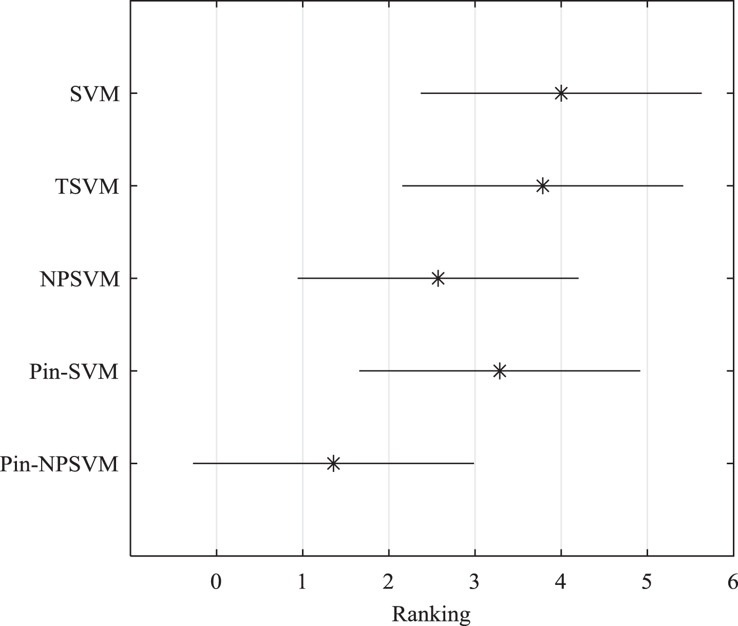The Friedman statistic can be calculated by (32), $χ_{F}^{2} = \frac{12 n}{t (t + 1)} [\sum_{j} {Rank}_{j}^{2} - \frac{t (t + 1)^{2}}{4}],$ (32) where, ${Rank}_{j} = \frac{1}{n} \sum_{i = 1}^{n} {rank}_{i}^{j},$ and ${rank}_{i}^{j}$ denotes the j^th of t algorithms on the i^th of n datasets. Friedman’s $χ_{F}^{2}$ is undesirably conservative and derives a better statistic $F_{F} = \frac{(n - 1) χ_{F}^{2}}{n (t - 1) - χ_{F}^{2}},$ (33) which is distributed according to F-distribution with (t-1) and (t-1) (n-1) degrees of freedom.

Fig. 1

Nemenyi test.

For the corrupted sets, the ranks of five linear algorithms in terms of accuracy are reported in Table 6. Table 6 shows that the average rank of our Pin-NPSVM is the lowest, which is equal to 1.357, and the average ranks of the other four algorithms are 4.000, 3.786, 2.571 and 3.286 respectively. The result justifies that our Pin-NPSVM is more effective than the other algorithms. To further testify the significant advantage of Pin-NPSVM, we calculate the values of the Friedman’s $χ_{F}^{2}$ and F_F according to (32) and (33). They are $χ_{F}^{2} = 25.67$ and F_F = 11, respectively. F_F is distributed according to F-distribution with (5–1) and (5–1) (14–1) degrees of freedom. When the level of significance α = 0 . 05, the critical value of F (4, 52) is 2.54. Because F_F = 11, which is much larger than the 2.54, α is less than 0.05. Hence, we can find that there is significant difference among five algorithms. In addition, in order to verify the significant difference between two algorithms, we adopt the Nemenyi test and the testing result is shown in Fig. 1, where * represents the average rank, and the line segment centered on the * refers to the critical range CD (CD = 1.63), where CD is calculated as the following ${CD}_{(a = 0.05)} = q_{α} \sqrt{\frac{t (t + 1)}{6 \times n}} = 1.63 .$ (34)

Table 6

Average rank of linear classifiers in the corrupted sets

Dataset	SVM	TSVM	NPSVM	Pin-SVM	Pin-NPSVM
Australian	4	5	2	3	1
Heart	5	4	2	3	1
Iris	5	3.5	1	3.5	2
Liverdisorder	2	4	5	3	1
Sonar	3	5	2	4	1
Vote	4	5	3	2	1
Wdbc	4.5	2	3	4.5	1
Wine	5	4	1	3	2
Wpbc	4	5	2	3	1
Haberman	4.5	3	1	4.5	2
Ionosphere	4	5	1	3	2
Diabetes	5	3	4	2	1
Blood	4	1	4	4	2
Balance	2	3.5	5	3.5	1
Average rank	4	3.786	2.571	3.286	1.357

5.2 ORL face dataset

ORL face dataset [30] is a common dataset, which is often applied to supervised learning. This dataset contains 400 face images made up of 40 people. Each person has 10 pictures of face with different details, lighting and expressions. The size of each picture is 119 × 92, and the gray level is 256. For each person, 5 pictures are selected as training samples and the rest as testing samples. So, there are 200 training samples and 200 testing samples. In order to test the robustness of the Pin-NPSVM, a corrupted face dataset is built by the zero-Gaussian noise with the variance of 0.05. Figure 2 shows a human face of the original and the corrupted sets, respectively. The first image is the original face, and the second is the corrupted face.

Fig. 2

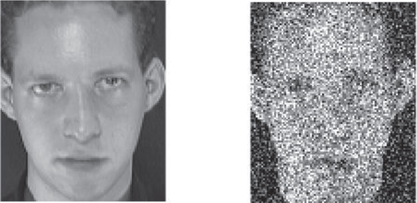
Examples in the original and corrupted ORL face sets.

In the experiment, seven classifiers are compared. In order to realize multi-class classification, SVM, NPSVM, TSVM, Pin-SVM and Pin-NPSVM are combined with binary tree. Both NMF and DT algorithms can realize multi-class classification by themselves. The original and the corrupted sets are processed before training. Because only the performance of seven algorithms is compared, the experiment is executed on the original pixel features. For the original and corrupted sets, the classification accuracies of seven classifiers are shown in Fig. 3.

Fig. 3

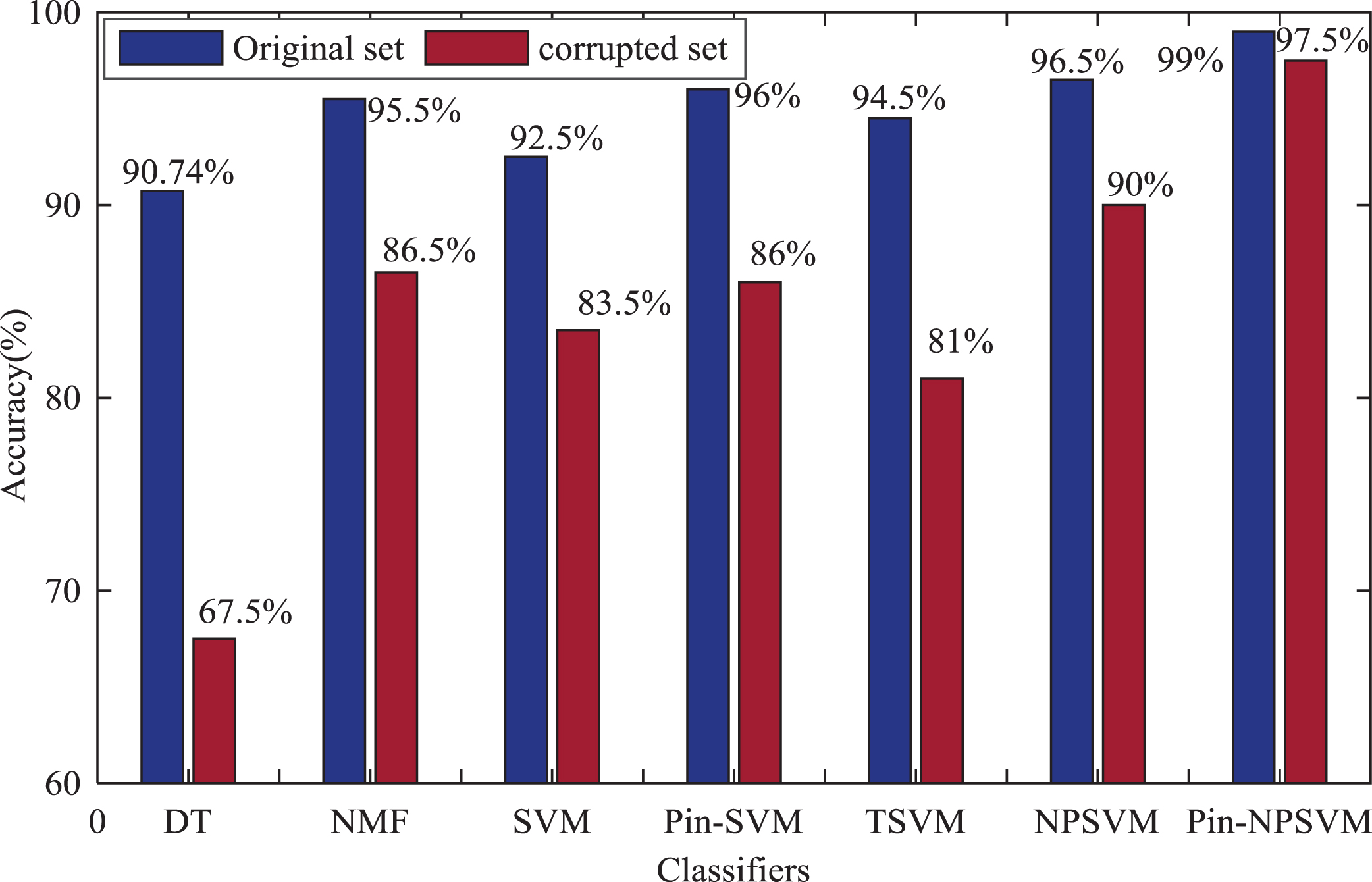
The testing results on the original and corrupted ORL face datasets.

By comparison, Pin-NPSVM and Pin-SVM yield better performance than other three SVM-based classifiers on the corrupted set. Meanwhile, the accuracy of Pin-NPSVM is higher than that of Pin-SVM. And, the classification accuracy of Pin-NPSVM on the corrupted set is slightly lower than that on the original set. It means that Pin-NPSVM is insensitive to noise. The reason is that the Pin-NPSVM has advantages of pinball loss and nonparallel structure. In addition, the NMF classifier is slightly better than SVM and TSVM in accuracy for the original and the corrupted sets, which shows that NMF classifier is more suitable for face recognition. But, for the corrupted set, NMF classifier couldn’t achieve good results, which implies that NMF is sensitive to noise. Moreover, it can be seen that the DT classifier is obviously affected seriously by the noise. The reason is that DT algorithm is less robust when the dataset is corrupted by noise.

5.3 Defects image datasets

To demonstrate the effectiveness of our Pin-NPSVM, we apply the Pin-NPSVM, NPSVM, TSVM, Pin-SVM, SVM and DT algorithms to steel surface defects datasets [31, 32]. In this experiment, six types of defects images are chosen, such as pitted-surface (PE), patches (PH), crazing (CG), inclusion (IN), scratches (SH) and rolled-in-scale (RE), which are shown in Fig. 4. These defects images are processed to obtain defects samples, and all defects samples form a defects samples set. The defects datasets include 3718 defects samples and each defect sample is a 18-dimensional vector.

Fig. 4

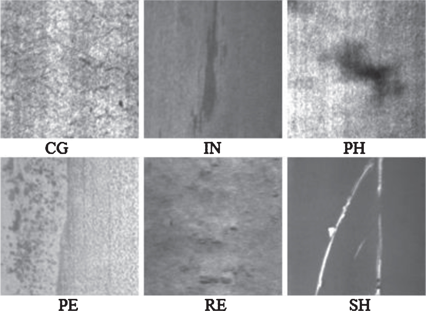
Six types of defect images.

To verify the robustness of our Pin-NPSVM, the features of the defects samples are corrupted by zero-mean Gaussian noise with variance of 0.05, forming the corrupted defects datasets. The comparative experiment is done on the corrupted defects datasets. The five SVM-based classifiers are combined with ”1 vs rest” method to realize the classification problem for multi-class defects datasets. DT algorithm itself can achieve multi-class classification. Table 7 shows the classification accuracies of the six classifiers in the defects datasets.

Table 7

The testing accuracies of six classifiers on defects datasets

Dataset	DT	SVM Accuracy (%)	TSVM Accuracy (%)	Pin-SVM Accuracy (%)	NPSVM Accuracy (%)	Pin-NPSVM Accuracy (%)
CG	93.28	88.06	88.06	85.07	87.37	97.31
IN	97.14	95.71	93.57	94.29	97.86	97.48
PH	98.86	95.86	97.93	98.62	97.24	100
PE	73.68	67.37	72.63	70.53	66.32	75.58
RE	95.12	95.12	96.75	96.75	95.12	97.50
SH	94.39	91.59	93.46	94.39	92.52	96.26
Total Accuracy	92.47	90.05	91.26	90.86	90.59	95.62
Average rank	2.75	4.92	3.83	3.83	4.67	1

From Table 7 we can learn that our Pin-NPSVM is always the best in accuracy for all types of defects datasets. And Pin-SVM has better performance than SVM with hinge loss. The result shows that the pinball loss can bring noise insensitivity. Moreover, the accuracies of Pin-NPSVM, NPSVM and TSVM are higher than those of SVM, which highlights that the nonparallel structure can enhance the generalization performance of the model. In addition, Pin-NPSVM and TSVM show better performance than NPSVM for the corrupted defects datasets, which implies that making full use of the prior structure information of data can improve the robustness of the model to noise samples. Furthermore, it can be seen that the DT algorithm is better than SVM, TSVM, Pin-SVM and NPSVM in accuracy. It shows that the DT algorithm is fit for the steel surface defects classification. In addition, we can also see that average rank of our Pin-NPSVM is the smallest among the all classifiers.

To further verify the superior performance of the Pin-NPSVM, the Friedmen test is adopted in this experiment. According to (32) and (33), we can have $χ_{F}^{2} = 16.141$ and F_F = 5.823. F_F is distributed according to F-distribution with 5 and 25 degrees of freedom. When the level of significance α = 0 . 05, the critical value of F (5, 25) is 2.603 Because F_F > F (5, 25), the p-value calculated by F (5, 25) is lower than 0.05, which highlights there is obvious difference between Pin-NPSVM and the other classifiers on the corrupted defects datasets. It further verifies that our Pin-NPSVM is more suitable for the classification of steel surface defects with feature noise.

6 Conclusion

In this paper, a novel Pin-NPSVM algorithm is proposed for pattern recognition. Pin-NPSVM has significant characteristics because of the pinball loss, the nonparallel structure and the prior structure information. Inspired by the Pin-SVM, the Pin-NPSVM is constructed by introducing the pinball loss into the NPSVM algorithm, which can ensure that Pin-NPSVM is insensitive to noise, especially for the feature noise around the decision boundaries. In addition, the Pin-NPSVM has better classification performance than Pin-SVM because of its nonparallel structure. Meanwhile, the prior structural information is considered for Pin-NPSVM, which can enhance the robustness of the model.

Finally, a large number of comparative experiments are carried out on the UCI datasets and image datasets to verify the effectiveness of the proposed Pin-NPSVM algorithm. The results show that the Pin-NPSVM holds better generalization performance than other state-of-the-art classifiers especially in solving the classification with noise. Moreover, it can be seen that there are at least four independent parameters in the Pin-NPSVM model. Too many parameters will affect the complexity of the model, so, we will focus on how to select the optimal parameters more effectively in the future.

Footnotes

Acknowledgment

The authors would like to thank the reviewers for helpful comments and suggestions. This work was supported by Natural Science Foundation of Liaoning Province, China (No. 20180550067), Liaoning Province Ministry of Education Scientific Study Project (No. 2017LNQN11) and University of Science and Technology Liaoning Talent Project Grants (No. 601011507-20 and No. 601013360-17).

References

Pernkopf

, Bayesian network classifiers versus selective k-NN classifier, Pattern recognition 38(1) (2005), 1–10.

Daga

, Shaikhina

, Lowe

, Briggs

and Khovanvoa

, Decision tree and random forest models for outcome prediction in antibody incompatible kidney transplantation, Biomedical Signal Processing & Control 37(10) (2017), 1025–1042.

T.K.

and Kim

M.H.

, A new diverse AdaBoost classifier, In, 2010 International Conference on Artificial Intelligence and Computational Intelligence 1 (2010), 359–363.

Guillamet

, Vitrià

and Schiele

, Introducing a weighted non-negative matrix factorization for image classification, Pattern Recognition Letters 24(14) (2003), 2447–2454.

, Wang

, Cheng

, Wu

, Gan

and Fang

, Cloud removal in remote sensing images using nonnegative matrix factorization and error correction, Isprs Journal of Photogrammetry & Remote Sensing 148 (2019), 103–113.

, Wang

, You

and Zhang

, Multiple Kernel Learning via Low-Rank Nonnegative Matrix Factorization for Classification of Hyperspectral Imagery, IEEE Journal of Selected Topics in Applied Earth Observations & Remote Sensing 8(6) (2015), 2739–2751.

Cortes

and Vapnik

, Support-vector network, Machine Learning 20(3) (1995), 273–297.

Vapnik

V.N.

, The nature of statistical learning theory, Springer Science & Business Media, 2013.

Richhariya

and Tanveer

, EEG signal classification using universum support vector machine, Expert Systems with Applications 106 (2018), 169–182.

10.

Fan

, Wang

, Li

, Gao

and Zha

, Entropy-based fuzzy support vector machine for imbalanced datasets, Knowledge-Based Systems 115 (2017), 87–99.

11.

Chu

, Liu

, Gong

and Liu

, Multi-class classification method using twin support vector machines with multi-information for steel surface defects, Chemometrics and Intelligent Laboratory Systems 176 (2018), 108–118.

12.

Suykens

J.A.

and Vandewalle

, Least squares support vector machine classifiers, Neural Processing Letters 9(3) (1999), 293–300.

13.

Mangasarian

O.L.

and Wild

E.W.

, Multisurface proximal support vector machine classification via generalized eigenvalues, IEEE Transactions on Pattern Analysis and Machine Intelligence 28(1) (2006), 69–74.

14.

Tax

D.M.J.

and Duin

R.P.W.

, Support vector data description, Machine Learning 54(1) (2004), 45–66.

15.

Jayadeva , Khemchandani

and Chandra

, Twin support vector machines for pattern classification, IEEE Transactions on Pattern Analysis and Machine Intelligence 29(5) (2007), 905–910.

16.

Peng

, A ν-twin support vector machine (ν-TSVM) classifier and its geometric algorithms, Information Sciences 180(20) (2010), 3863–3875.

17.

Kumar

M.A.

and Gopal

, Least squares twin support vector machines for pattern classification, Expert Systems with Applications 36(4) (2009), 7535–7543.

18.

Shao

Y.H.

, Zhang

C.H.

, Wang

X.B.

and Deng

N.Y.

, Improvements on twin support vector machines, IEEE Transactions on Neural Networks 22(6) (2011), 962–968.

19.

Ghorai

, Mukherjee

and Dutta

P.K.

, Nonparallel plane proximal classifier, Signal Processing 89(4) (2009), 510–522.

20.

Guyon

, Matic

and Vapnik

, Discovering Informative Patterns and Data Cleaning, (1996), 181–203.

21.

Herbrich

and Weston

, Adaptive Margin Support Vector Machines for Classification, (1999), 880–885.

22.

Zhang

J.H.

and Wang

Y.Y.

, A rough margin based support vector machine, Information Sciences 178(9) (2008), 2204–2214.

23.

, Tian

and Shi

, Robust twin support vector machine for pattern classification, Pattern Recognition 46(1) (2013), 305–316.

24.

Huang

, Shi

and Suykens

J.A.K.

, Support vector machine classifier with pinball loss, IEEE Transactions on Pattern Analysis & Machine Intelligence 36(5) (2014), 984–997.

25.

Lee

D.D.

and Seung

H.S.

, Learning the Parts of Objects by Non-Negative Matrix Factorization, Nature 401(6755) (1999), 788–791.

26.

Almuallim

, An efficient algorithm for optimal pruning of decision trees, Artificial Intelligence 83(2) (1996), 347–362.

27.

Dua

and Taniskidou

E.K.

, UCI Machine Learning Repository, [Online]. Available: http://archive.ics.uci.edu/ml/

28.

Demšar

, Statistical comparisons of classifiers over multiple data sets, Journal of Machine Learning Research 7 (2006), 1–30.

29.

Nemenyi

, Distribution-free Multiple Comparisons. URL https://books.google.fi/books?id=nhDMtgAACAAJ

30.

Olivetti, ORL Faces Database. [Online]. Available: http://www.uk.research.att.com/facedatabase.html

31.

, Song

, Meng

and Yan

, An End-to-End Steel Surface Defect Detection Approach via Fusing Multiple Hierarchical Features, IEEE Transactions on Instrumentation and Measurement 69(4) (2020), 1493–1504.

32.

Dong

, Song

, He

, Xu

, Yan

and Meng

, PGA-Net: Pyramid Feature Fusion and Global Context Attention Network for Automated Surface Defect Detection, IEEE Transactions on Industrial Informatics.

A nonparallel support vector machine with pinball loss for pattern classification

Abstract

Keywords

1 Introduction

2 Brief introduction to NPSVM

3.1 Pinball loss

5 Experiments

5.1 UCI datasets

Table 1 The attributes of UCI datasets Dataset Feature Data Class Australian 14 690 2 Heart 12 270 2 Iris 4 150 3 Liverdisorder 6 345 2 Soner 60 208 2 Vote 16 435 2 Wdbc 30 569 2 Wine 12 178 2 Wpbc 33 198 2 Haberman 3 306 2 Ionosphere 34 351 2 Diabetes 8 768 2 Blood 4 748 2 Balance 4 625 3

Footnotes

Acknowledgment

References