






Abstract
The purpose of this paper is to solve the portfolio selection problem when historical data are unavailable. In this paper, the problem is viewed as a multi-criteria decision making (MCDM) problem under intuitionistic fuzzy circumstances, and the prospect theory is utilized to reflect decision makers’ psychological state, which is always bounded rational. Therefore, a new approach to solve MCDM problems is presented based on the following improvements. (a) The entropy-weighted method with extreme data resistance is proposed instead of weight function to deal with the weight of criteria, because weight stands for the decision maker’s preference of criteria rather than objective probability and should not be distorted. (b) A new entropy-weighted method with confidence degree is presented, which can not only describe the uncertainty of information each criterion provides but also reflect the decision maker’s confidence in the information. (c) To reduce the interference from extreme data, the median is selected as reference point instead of mean or extreme value. (d) Based on the distance measure, the intuitionistic fuzzy prospect value function is presented to capture decision makers’ psychological state. Finally, a novel model with prospect value constraint and risk preference is constructed to allocate investment ratios. For our proposed method and model, two numerical applications are given to verify their validity and the sensitivity analysis is carried out to illustrate their practical significance.
Keywords
Introduction
It is doubtless that the modern portfolio selection theory [1] is one of the most outstanding breakthroughs in the field of portfolio selection because it introduced a new way to solve the portfolio problem by using mathematical tools. As its founder, Markowitz won the Nobel Prize in 1990, which underlines the excellence of this achievement. After that, based on the mean-variance probabilistic model proposed in his theory, more and more diversified models have developed by the researchers to fit in with the complicated financial market nowadays. Most of these models are built on the assumption that stock returns can be described as stochastic variables so that we can denote the returns and risks of portfolio by a set of numbers to make the process clearer. For example, Li and Ng [2] proposed a multi-period mean-variance model for dynamic portfolio selection; Leippold et al. [3] presented a geometric approach to discrete time multi-period mean variance portfolio optimization and gave a simpler interpretation for the model in mathematics and economics; Liu [4] solved the portfolio selection problem when the asset returns are quadratic and the investor has a constant relative risk aversion coefficient; Harvey et al. [5] put forward a method for optimal portfolio selection based on the Bayesian decision theoretic framework to handle the higher moments and parameter uncertainty, which are the major shortcomings of the traditional Markowitz approach; Wong et al. [6] held a comprehensive study of the utility-deviation-risk portfolio selection problem and pointed out that semi-variance could be regarded as a proper risk measure in the classical portfolio management paradigm; Seng and Ying [7] studied the mean-variance (MV) portfolio problems under static and dynamic settings and put forward the linear programming optimal portfolio, which outperforms the equally weighted portfolio and the estimated optimal portfolios using shrinkage and other competitive estimators.
As mentioned above, conventional portfolio selection theory is based on the premise that the future return and risk of portfolio can be always predicted only by relying upon the historical data and be considered as the numerical characteristics of specific stochastic variables. Nevertheless, it is difficult for us to collect the precise data of some stocks in all time due to the complicated and ever-changing circumstances of the financial market. On the other hand, if there are some newly listed stocks that the investor prefers to invest in, the conventional method will not able to offer him/her a satisfactory solution. Thus, it is necessary to find a new way to address these problems. In fact, considering the similarity between the above problem and the multi-criteria decision making (MCDM) problem, it is an effective method to treat the problem as an MCDM problem and then obtain an acceptable solution. MCDM problem generally provides the decision maker some assessments of the alternatives under several quantitative or qualitative criteria and then requires him/her to make a ranking of these alternatives. Although it also relies on the past data to some degree, its demand for data is comprehensive rather than highly rigorous. Thus, it is more flexible and adaptive than the conventional method. In recent years, the research of MCDM problem has attracted great attention: Wu and Zhang [8] proposed the concept of intuitionistic fuzzy weighted entropy and established the programming model to generate optimal weight of criteria to solve MCDM problem according to the minimum entropy principle; Joshi and Kumar [9] proposed an intuitionistic fuzzy TOPSIS method for MCDM problem to rank the alternatives based on distance measure and intuitionistic fuzzy entropy; Chen and Chang [10] studied the transformation techniques between intuitionistic fuzzy values and right-angled triangular fuzzy numbers and then proposed some intuitionistic fuzzy geometric averaging operators for fuzzy MCDM problem; Jia and Zhang [11] solved the MAGDM problem in which all information is characterized by interval-valued intuitionistic fuzzy number and the information about the weights of both decision makers and attributes may be completely unknown or partially known.
Fuzzy set theory, proposed by Zadeh [12] in 1965, is frequently utilized in MCDM problem for the assessments of alternatives due to its powerful ability to deal with uncertainty information. Unlike traditional set theory, fuzzy set theory adopts a continuous variable with the range [0, 1] rather than an indicator variable, which can only express the status by integer 0 or 1, to describe the membership degree of an element belonging to a set. It is apparent that fuzzy set is more flexible than traditional set. On this basis, Atanassov [13] extended the fuzzy set theory to intuitionistic fuzzy set theory by introducing the non-membership degree of element. Thus, intuitionistic fuzzy set (IFS) can describe uncertainty information from both positive and negative perspectives, which makes it more efficient and practicable than fuzzy set. For this reason, many researchers suggested that IFS should be widely applied in technical fields, such as pattern recognition [14, 15], medical diagnosis [15, 16] or risk assessment [17]. Similarly, it could be found that IFS plays an increasingly important role in MCDM problem. Mao et al. [18] studied the cross-entropy and entropy measures of IFSs and provided an example to show their application in MCDM problem; Wang [19] did the research on the MCDM problem with intuitionistic fuzzy preference relation; Tao and Witold [20] put forward a novel model for MCDM problem based on an intuitionistic fuzzy weighted arithmetic average operator; Wu et al. [21] adopted the triangular intuitionistic fuzzy numbers to cope with the uncertainties and proposed an intuitionistic fuzzy multi-criteria framework; Combined with the set pair analysis (SPA) theory, Garg and Kumar [22] proposed a family of distance measures based on the Hamming, Euclidean, and Hausdorff metric for connection number set, and they solved the MCDM problem under IFS environment based on these distance measures; By using the connection number of the SPA theory, Garg and Kumar [23] presented some new similarity and weighted similarity measures of IFS and then utilized these measures to solve MCDM problem; Harish and Jaspreet [24] defined an (R, S)-norm-based information measure called the entropy to measure the degree of fuzziness of IFS, which is used to propose two decision-making approaches to solve the MCDM problem under IFS environment; Garg and Kumar [25] presented some exponential based distance measures using connection numbers of the interval-valued intuitionistic fuzzy sets (IVIFs) to enrich the theory of information measure, and then developed a TOPSIS method based on these distance measures to solve MCDM problem under IVIF environment.
Apart from the uncertainty under complicated circumstances, there is another factor that may affect the decision maker’s preference in MCDM problem. Conventional MCDM method based on the premise that the decision maker is completely rational, so that he/she can makes decision just by relying on the assessments of each alternative. However, it is difficult for the decision maker to keep completely rational when he/she knows some information about the alternatives, and then his/her psychological state would affect the decision result. To illustrate this condition, some researchers studied the behavioral decision making problem and then developed some outstanding theories. One of these outstanding theories is the prospect theory, which was proposed by Kahneman and Tversky [26] in 1979, for it provided a successful explanation of some unreasonable financial behaviors. Without question, it became a critical tool to reflect the decision maker’s psychological state and was widely applied to MCDM problem. Liu et al. [27] researched MCDM problem under risk with interval probability based on prospect theory and the uncertain linguistic variables; Renato and Talles [28] proposed a hybrid approach combining prospect theory and fuzzy numbers to handle risk and uncertainty in MCDM problems; Wang et al. [29] combined the score function and prospect theory to solve the interval-valued intuitionistic fuzzy MCDM problem; Zhu et al. [30] considered multiple reference points in decision making to make the solution more effective and adaptive; Tian et al. [31] presented the definition of intuitionistic fuzzy prospect value and applied it to MCDM problem to choose a promising enterprise for venture capitalists; To guarantee the effectiveness of information aggregation and to extend the feasibility of prospect theory, Jia and Wang [32] proposed a novel decision-making approach based on rough numbers and prospect theory to solve risky and uncertain MCDM problems.
Unfortunately, although Wang [29] and Tian [31] attempted to introduce the prospect theory into IFS theory, their methods still have some drawbacks. Wang just put emphasis on the score function but ignored the fundamental differences of IFSs, and Tian utilized IFSs in the weighting function instead of the assessments for alternatives. In addition, most of the researchers adopted the weighting function to distort the weights of each criterion, and they did not realize that weight is not the probability but the decision maker’s preference for criteria. Thus, it is unnecessary to use the weighting function.
In order to overcome the above drawbacks and better reflect the rational degree of the investor in decision making process (As mentioned above, decision maker cannot keep complete rationality in that process), in this paper, we do the following works: The entropy-weighted method is introduced to deal with weights of criteria rather than weighting function for the first time. In addition, this method is improved in the aspect of resistance to extreme data and then extended to reflect the decision maker’s confidence degree in all the information he/she holds. It has been proved that the improved method is more flexible and practical than the conventional one; To reduce the interference from extreme data, the median is selected as reference point instead of mean or extreme value. And then, the distance measure is introduced into the prospect value function to better describe the deviation between IFSs; On these bases, a novel model with prospect value constraint is presented to solve the above portfolio selection problem according to the investor’s risk preference. The advantage of our model is that it can flexibly reflect the investor’s degree of rationality. Also, the sensitivity analysis of different rational degree and risk preference is carried out.
The rest of this paper is organized as follows. In Section 2, some basic conceptions of IFS theory and prospect theory are provided. In Section 3, the conventional entropy-weighted method is modified and extended to reflect the decision maker’s confidence degree. The intuitionistic fuzzy prospect value function based on distance measure is defined and a novel portfolio selection model with prospect value constraint is presented in Section 4. In Section 5, a numerical application is given to illustrate the effectiveness of the proposed model and the sensitivity analysis is carried out. Finally, the conclusion is drawn in Section 6.
Preliminaries
In this section, some basic conceptions of IFS theory and prospect theory will be briefly mentioned for the following sections.
The intuitionistic fuzzy set theory
It should be noted that the membership function μ
A
(x) and non-membership function ν
A
(x) should satisfy μ
A
(x) + ν
A
(x) ≤ 1. Thus, let π
A
(x) = 1 - (μ
A
(x) + ν
A
(x)), we have 0 ≤ π
A
(x) ≤ 1, ∀x ∈ X. π
A
(x) is called the hesitancy degree of x to IFS A, and then A can also be denoted as follows:
For the sake of convenience, in this paper, we use IFS (X) to denote the set of all IFSs in the universe of discourse X.
It is not difficult to find that
It is not difficult to find that
If If If
Entropy is one of the measures which can describe the uncertain degree of IFS. The greater the value of entropy is, the greater the uncertainty is. In this paper, we will use it to assign the weights to each criterion by the entropy-weighted method [36].
The intuitionistic fuzzy entropy proposed by Wei et al. [37] is introduced as follows:
Obviously, we have E (A) ∈ [0, 1].
Distance measure is another important role in IFS theory, for it can describe the deviation between two IFSs. The larger the distance is, the greater the deviation is. In this paper, we adopt the distance measure proposed by Jiang et al. [38] to measure the deviation between two IFSs because it can avoid the shortcomings of most existing measures.
Prospect theory provides appropriate explanations for some irrational behaviors of human being, such as disposition effect and loss aversion in portfolio selection. Prospect theory points out that decision maker’s prospect value is not dependent on the total outcomes of the alternatives but the gains or losses relative to the reference point. In addition, it stresses that decision makers are sensitivity decreasing, that is, with the increase of gains or losses, their sensitivity as to the same change of gains or losses diminishes.
Except for the above phenomena, prospect theory also claims that decision maker often holds an incorrect perception on the event probability. Particularly, decision maker tends to overestimate the lower probability but underestimate the higher probability. Thus, Tversky and Kahneman [39] defined the weighting function on event probability.
Based on Tversky and Kahneman’s empirical research [39], the parameters in Equation (8) and Equation (9) are determined as: α = β = 0.88, λ = 2.25, γ = 0.61 and δ = 0.69.
As we mentioned in the introduction, some researchers adopted the weighting function to distort the weights for criteria when they combined prospect theory with fuzzy theory in the decision making process. This is not sensible enough because weights represent the decision maker’s preferences for each criterion, rather than the subjective cognition to objective event probability. In brief, it is unnecessary to distort the decision maker’s preferences. Hence, in this paper, we will use entropy-weighted method instead of weighting function to allocate weights for each criterion. Nevertheless, conventional entropy-weighted method lacks the resistance to extreme data and would provide the decision maker inappropriate weights. To overcome its drawback, in this section, a novel entropy-weighted method is proposed and some properties are discussed.
The drawback of the entropy-weighted method and its modification
Since entropy denotes the uncertain degree of information, for a criterion, the smaller the entropy, the more the information it provides. Thus, the smaller the entropy of the criterion, the larger the weight it should possess. The conventional entropy-weighted method is presented based on this principle, and it can be illustrated as:
Suppose C ={ C1, C2, ⋯ , C
n
} is a set of criteria, E ={ E1, E2, ⋯ , E
n
} is a set of entropy, where E
i
denotes the entropy of C
i
, i = 1, 2, ⋯ , n. According to the conventional entropy-weighted method, the weight w
i
for C
i
can be calculated by the following equation:
For the convenience of discussion, let’s focus on the following examples.
The novel entropy-weighted method is defined as follows:
There are some properties for the novel entropy-weighted method:
When E
j
≥ 0.7, that is, 1 - E
j
≤ 0.3, we can get When E
j
≤ 0.05, we have
To demonstrate the effectiveness and superiority of our proposed method, some cases are presented and the corresponding results are show in Table 1, where w
j
denotes the weight allocated to criterion C
j
calculated by the conventional method and
The entropy and weights of criteria
1The numbers in bold denote that the corresponding weights are not suitable enough in decision making process.
From Table 1, we can find that: In Case 1 and Case 2, our method is as effective as the conventional one. Even in Case 1, the differences among weights calculated by the proposed method are smaller and more appropriate. In Case 3, the weights calculated by our method is average and more rational than those of the conventional one. In Case 4, the differences between the weights calculated by our method are less than those obtained by the conventional method, which implies that our method is more resistant to extreme data.
In conclusion, the proposed method is more feasible and adaptive than the conventional entropy-weighted method in practice.
In 3.1, we point out that the entropy represents the uncertainty of information a criterion provides. On this basis, considering that in the decision making process, it is common that the decision maker cannot ensure the information he/she knows about is completely accurate. Thus, when the decision maker has sufficient confidence in all the information he/she knows about, he/she may put more emphasis on the role of entropy and would like to make the differences of weights for each criterion more distinct. Conversely, he/she would like the difference to be less.
There is an example to directly explain the difference between entropy and confidence degree:
A man wants to choose a primary school for his daughter to study in, and he has several alternatives. To ensure that his daughter can study in a better environment, this man has consulted an expert and got some advice. However, for the complexity of the problem (There is no single criterion that can comprehensively assess the quality of a school), and the limitation of the expert’s cognition, these pieces of advice include uncertain information to some extent, which is called entropy if we quantify the uncertain degree.
In addition, this man has his own judgment on the advice. If he completely trusts the expert, he would put more attention to the advice that has less uncertainty; if he has little trust of the expert, he may neglect all the advice no matter how uncertain they are. In this case, it can be regarded that there are no difference in these pieces of advice. We quantify the man’s trust in the expert, which can be seen as his confidence degree on the advice.
From this example, it is not difficult to find out that entropy represents the uncertainty of the information itself, while confidence degree points out the decision maker’s trust in the source of information, which is irrelevant to the uncertain degree of the information itself.
In order to incorporate the confidence degree into our method to make it more flexible, a novel entropy-weighted method with confidence degree is presented as follows:
How to determine the value of γ is expressed in Remark 2. Before that, let us focus on the following theorems of Equation (13):
then, for i∉ { m1, m2, ⋯ , m p },
we have E i - Emin > 0 and γE i -Emin→ + ∞, γEmin-E i → 0+ (γ → + ∞).
In addition, for j∈ { 1, 2, ⋯ , n }, we have γE i -E j ≥ 0 (γ ≥ 1),
thus, .
For k∈ { m1, m2, ⋯ , m p }, we have E k - Emin = 0 and, by γEmin-E i → 0+ (γ → + ∞),
then,
In summary, we have
It is illustrated in property 2 that if the decision maker is extremely unconfident about the information he/she holds, he/she would like to allocate each criterion the same weight rather than that calculated by the entropy. Conversely, property 3 tells us that if the decision maker is overconfident, he/she will just choose the best criteria, which provide the most information to make decision. And property 1 establishes a connection between the above two properties, which implies that the larger the value of γ is, the more confidence the decision maker holds.
This analysis demonstrates that the novel entropy-weighted method with confidence degree has great decision making significance and is in line with the practice. In Section 5, we will do more analyses about the different values of γ.
In practical portfolio selection, it is impossible to require the investor to keep completely rational in all time, especially when the investor has known some information about the investments. To offer the investor satisfactory returns and reduce risks to an acceptable level, while providing the investor enough sense of achievement, in this section, the prospect theory is combined with the intuitionistic fuzzy set theory, and then, as one kind of MCDM problem, a new type of model is constructed for portfolio selection under intuitionistic fuzzy circumstances.
The selection of the reference point
According to prospect theory, the investor’s prospect value depends on the reference point. Therefore, it is essential to determine the reference point at the beginning. However, we should notice that the selection of reference point is critical to the prospect value function, thus it should be treated deliberately. Look back on some existing researches, we can find that most of the researchers adopted mean value, maximum value or minimum value as reference point. Although these reference points represent kinds of economic implications, it should not be overlooked that they are vulnerable to extreme data. The following example is given to explain this problem.
The grades of each project
The grades of each project
From Table 2, we obtain the average score of these projects is 80.29, and the maximum score among them is 97. Whether we use the mean value or the maximum value as reference point, we would obtain a series of negative prospect value for all the projects, besides A3, the best project with the highest score. It is undoubtedly terrible and may severely reduce the investor’s desire to invest. Even that minimum value is a proper choice in this case, it may be invalid in other conditions.
To solve the above problem, we adopt the median as reference point. In Example 3, the median of the scores is 78, which is obviously better than the mean value and the maximum value as a reference point.
In fact, median is a statistic with excellent properties. Since it is little affected by extreme data and can describe the distribution of the data to some extent, thus, in this paper, we will adopt median as the reference point and then constructed the intuitionistic fuzzy prospect value function.
As we introduced in Section 2, prospect value is comprised of three parts: weighting function, reference point and prospect value function. The first two parts have been discussed above. Next, we will consider the form of prospect value function under intuitionistic fuzzy circumstances.
Suppose there are several projects A1, A2, ⋯ , A
n
that the investor is interested in and plans to invest in. Based on the information the investor holds, each project is scored in intuitionistic fuzzy number form as
Considering that the decision maker’s risk aversion degree will be reduced when we use median rather than extreme value as the reference point, in this paper, we will set α = β = 0.88 and λ = 1.5 in the following models.
In order to analyze the relationship between prospect value and distance measure more conveniently in Section 5, the positive prospect value and negative prospect value are defined as follows:
Obviously,
Suppose there are several projects A1, A2, ⋯ , A
n
that the investor is interested in and plans to invest in. Since the historical data is lost and incomplete, the investor regards this portfolio selection problem as a MCDM problem, and intends to assess the projects under some criteria to draw an investment programming. If C1, C2, ⋯ , C
m
are the criteria the investor has chosen (To be convenient, assuming that all the criteria are benefit type),
Considering that d
ij
represents the distance between
Since it is natural for the investor to pursue higher returns and lower risks, a portfolio selection model with prospect value constraint can be established as follows:
Apparently, θ reflects the investor’s degree of rationality, the larger the value of θ is, the more prospect value the investor pursues, which implies that the investor is more irrational.
It can be pointed out that Model (23) is equal to the following model:
To solve Model (25), we introduce the investor’s risk preference into the model and then transform it into the following single objective linear programming form:
Without question, we have μ ∈ [0, 1] in Model (26). From the practical significance, it can be viewed that μ is a lower bound of the investor’s satisfactory degree on returns. Correspondingly, δμ is a lower bound of the investor’s satisfactory degree on risks. Therefore, we can draw the following conclusions: The larger the parameter δ, the more the investor’s risk aversion willing. When δ > 1, the investor is profit-seeking; When δ = 1, the investor is neutral; When δ < 1, the investor is risk averse.
In Section 5, we will discuss the role of δ with different values.
As illustrated in Fig. 1, the process of our proposed method to address the portfolio selection problem under intuitionistic fuzzy circumstances can be simply listed as follows: Gain the assessments of each investment under the given criteria. Find out the medians as the reference points for each criterion. Obtain the entropy of each criterion by Equation (6) and then assign the weights to criteria by using the proposed entropy-weighted method shown in Equation (13). Calculate the distances between the investments and the reference points under each criterion by Equation (7). Calculate the positive distances and negative distances of each investment by Equations (19) and (20). Calculate the total prospect value of each investment by Equations (15) and (18). Allocate the investment ratios by Model (26) according to the investor’s risk preference and rational degree.

The process of portfolio selection under intuitionistic fuzzy circumstances.
Case I
Assuming that there are some companies that hold new projects and are looking for investment, and an investor is interested in these projects so that he/she plans to choose part of them to invest. Since the projects are newest and there is not any historical data to refer to, the investor decides to carry out some market research and consult the experts in related fields. After that, the investor has chosen six projects and then evaluated their companies according to the following six criteria: high market share (C1), good business performance (C2), high reputation (C3), rich experience in relevant fields (C4), excellent management team (C5), and the important position for the project (C6). Obviously, all the criteria are benefit type. For convenience, A1, A2, ⋯ , A6 are used to denote the companies and C1, C2, ⋯ , C6 are used to denote the criteria. The assessments of each project are listed in Table 3.
The assessments of each project in intuitionistic fuzzy number form
The assessments of each project in intuitionistic fuzzy number form
By calculating the scores and accuracy of each assessment by Equations (4) and (5), and ranking the assessments under the same criteria according to Definition 5, we can find the reference points of each criterion as follows:
By using Equation (6), the entropy of each criterion is obtained. To determine the value of parameter γ in Equation (13), we can refer to Remark 2. Without loss of generality, γ is taken as Euler number, that is, Equation (12) is adopted. And then, to make comparison, we also adopt the conventional entropy-weighted method to allocate weights for each criterion. The results are shown in Table 4 and Fig. 2. For convenience, E (C
j
) is used to denote the entropy of C
j
, w
j
and
The entropy and weights of each criterion
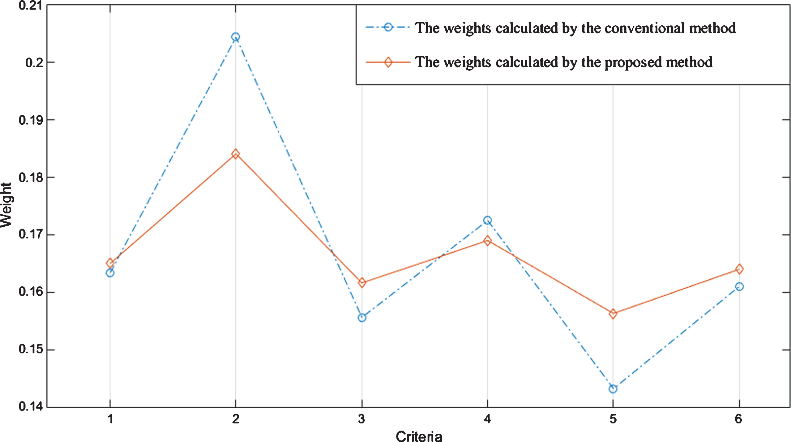
The weights of each criterion.
From Table 3 and Fig. 2, we can find that with the increase of w
j
,
After determining the weights, the positive distances and the negative distances of each project can be gained by Equations (19) and (20), and so are the positive prospect values and the negative prospect values. Here, we denote the positive distance and negative distance of A
i
as D1 and D2, the positive prospect value and the negative prospect value of A
i
as V1 and V2 when we use w
j
as the weight of criteria C
j
, respectively, V = V1 - V2. Similarly,
The positive distances and negative distances of each project
The positive prospect values and the negative prospect values of each project with α = β = 0.88, λ = 1.5
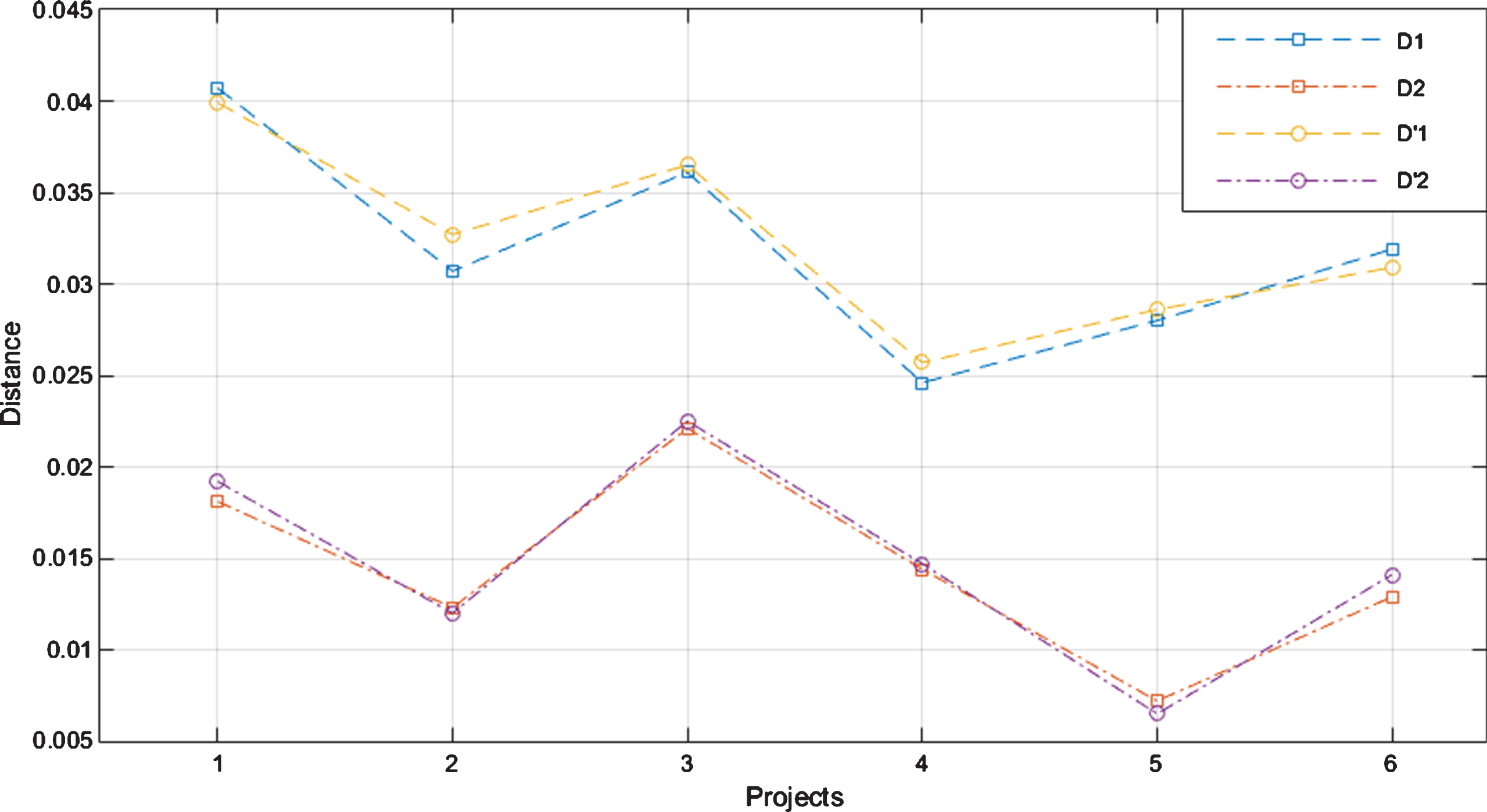
The positive distances and negative distances of each project.
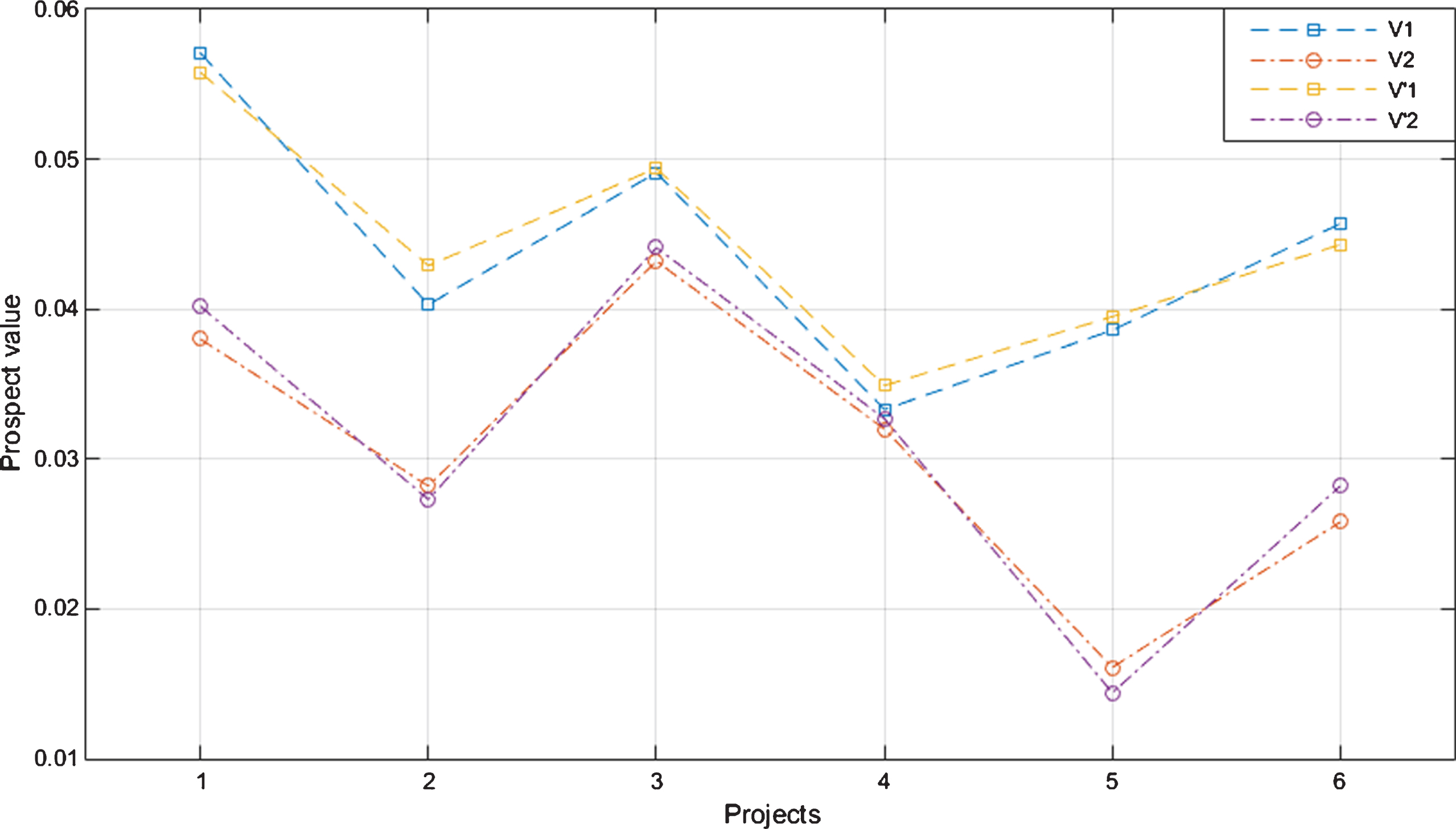
The positive prospect values and the negative prospect values of each project with α = β = 0.88, λ = 1.5.
From Figs. 3 and 4, we can find that: In Fig. 3, there are little differences in the shapes of D1 and By comparing Fig. 3 with Fig. 4, it is apparently that the shapes of D1 and V1, Whether in Fig. 3 or in the Fig. 4, the positive values are higher than the negative values, indicating that all the projects have performed well.
Since the effectiveness of our proposed entropy-weighted method is demonstrated, in the following model, we will adopt
If the investor wants to invest in each project at least 5 percent of the total investment, the constraint domain D can be set as
Let
Without loss of generality, suppose that the investor’s irrational degree is 50%, that is, θ = 0.5 (See the analysis in Section 5.3.2 for other conditions). In this condition, according to the investor’s different risk preferences, such as completely profit-seeking (δ = 0.5), slightly profit-seeking(δ = 0.75), neutral(δ = 1), slightly risk averse(δ = 1.25) or completely risk averse(δ = 1.5), the optimal solutions of Model (27) are obtained respectively and shown in Tables 7, 8 and Fig. 5.
The optimal investment ratios of each project with different risk preferences
The values of D+ (X), D- (X), V (X), D′+ (X) and D′- (X) with different risk preferences

The positive distance, negative distance and prospect value of portfolio.
From Tables 7, 8 and Fig. 5, we can find that: In Table 7, A1 and A5 are allocated the most investment ratios whatever the investor’s risk preference is, which underlines that these two projects are the best among all the projects. However, with the increase of δ, the investment ratio allocated to A1 decreases while that of A5 increases. Looking back on Table 5, we can find out the reason is that the negative distance of A5 is less than that of A1, which is critical when the investor tends to be risk averse. In Table 8, with the increase of δ, the value of D′+ (X) decreases while the value of D′- (X) increases. In fact, D′+ (X) and D′- (X) can be viewed as the investor’s satisfactory degree on returns and risks, respectively. Since the investor tends to be risk averse, he/she will put more emphasis on risks rather than returns, which is the cause for the change of D′+ (X) and D′- (X). In addition, when δ < 1, we have D′+ (X) > D′- (X), and when δ > 1, we have D′+ (X) < D′- (X), which is in line with the role of δ. In Fig. 5, it is distinct that the positive distance and the negative distance have the identical change trends, which points out that return is always in line with risk again. Nevertheless, the total prospect value has a completely contrary trend with the positive distance and the negative distance. In fact, since there is α = β = 0.88 in the prospect value function and the investor’s risk aversion degree λ = 1.5 is higher than 1, thus, decreasing a unit of risks can bring the investor more prospect value than increasing a unit of returns, which is the cause of the above phenomenon when δ increases.
Suppose there are five newly listed stocks A1, A2, ⋯ , A5 on the New York Stock Exchange, and an investor plans to invest in these stocks. Due to the insufficient historical data, it is difficult to obtain the probability/possibilistic distributions of returns of these stocks. Thus, the investor consults four professional evaluation agencies and obtains sufficient information about the stocks. All the information is shown in Table 9, where C1, C2, C3, C4 represent different evaluation agencies.
The assessments of each project in intuitionistic fuzzy number form
The assessments of each project in intuitionistic fuzzy number form
From Table 9, we can find that the assessment provided by C4 is generally higher than others and the assessments provided by C1 and C3 are generally lower. It can be inferred that the evaluation agency C4 holds an optimistic attitude towards these stocks and C1, C3 are relatively conservative.
According to Definition 5, the reference points (median) of each criterion are:
The entropy of each criterion is calculated by Equation (6). And then, according to Remark 2, we take γ = 5 to allocate weights for each evaluation agency (criterion) because the investor has enough confidence in the information. To make comparison, the conventional entropy-weighted method is also adopted. The results are shown in Table 10. For convenience, E (C
j
) is used to denote the entropy of C
j
, w
j
and
The entropy and weights of each criterion
From Table 10, we can find that with the increase of E (C
j
), w
j
and
Combined with the analysis in Section 3, it can be pointed out that our method is better than the conventional one. Thus, we will use
Since the weight of criteria is given, we can calculate the positive distances, the negative distances, the positive prospect values and the negative prospect values of each stock. Here, the positive distance and negative distance of A i are denoted as D1 and D2, the positive prospect value and the negative prospect value of A i are denoted as V1 and V2, and the corresponding total prospect value is V = V1 - V2. The results are shown in Table 11 and Fig. 6.
The distances and the prospect values of each stock with α = β = 0.88, λ = 1.5
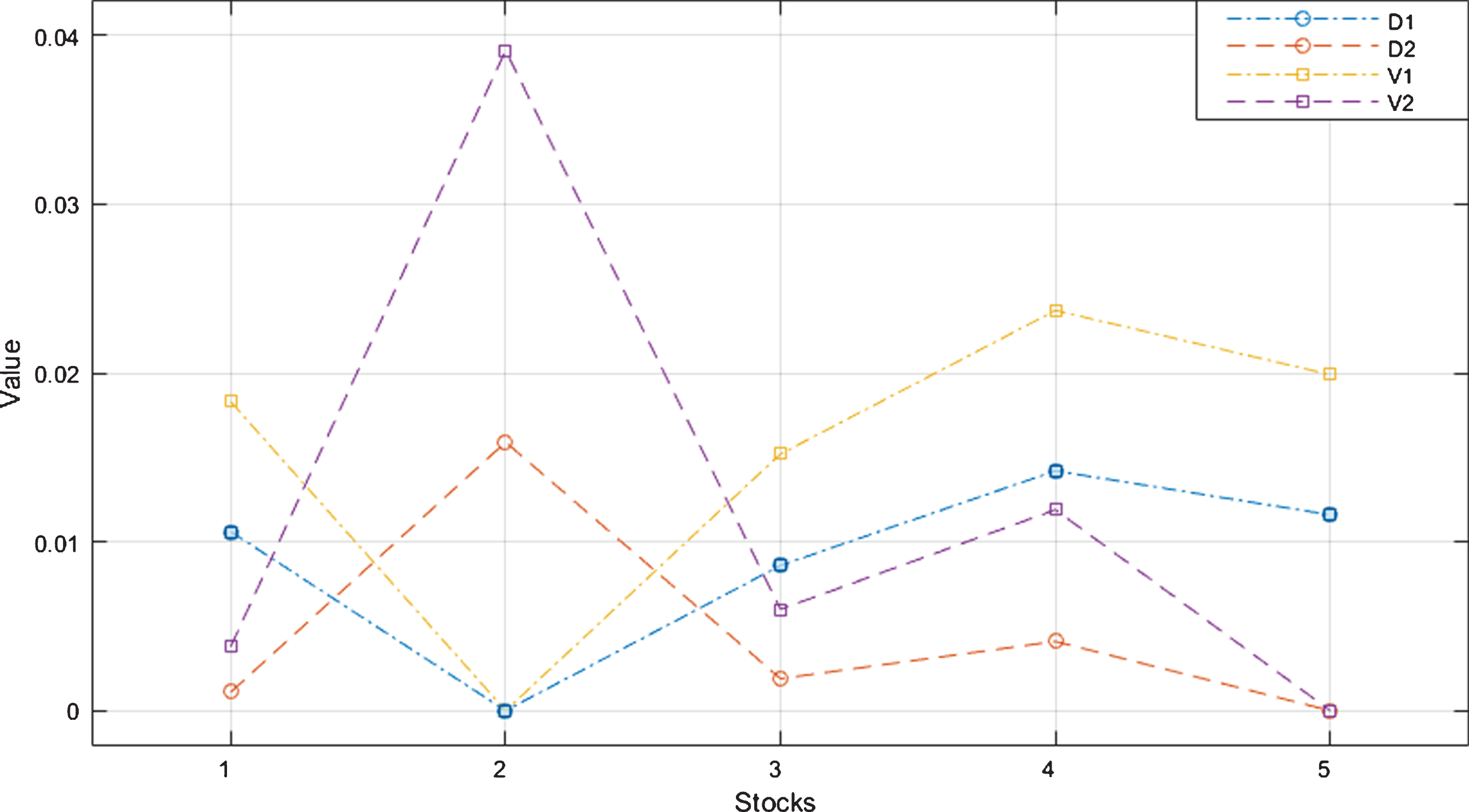
The distances and the prospect values of each stock with α = β = 0.88, λ = 1.5.
From Table 11 and Fig. 6, we can find that: The positive distance of A2 and the negative distance of A5 are zero. It does not mean that A2 cannot provide any return and A5 will not bring any risk. In fact, the positive distance describes the positive deviation between A2 and the reference point. Thus, when the distance is zero, the relative gains of A2 is zero. It’s the same for A5. According to Equation (8), it is not difficult to find that the positive prospect value of A2 and the negative prospect value of A5 are also zero. With the increase of positive/negative distances, the positive/negative prospect values increase. It is reasonable because a higher relative gain/loss will give the investor a higher positive/negative prospect value. The change of positive/negative prospect value is more drastic than that of positive/negative distance. The reason is that all the values of positive/negative distance are less than 1 and we take α = β = 0.88 < 1 in the intuitionistic fuzzy prospect value function. In this case, it is easy to find that a small change of relative gain/loss will lead to a big change of prospect value. In Table 11, we can find the total prospect value of A2 is negative. It means that A2 may bring more risks than benefits in the investor’s subjective cognition.
If the investor wants to invest each stock at least 10 percent of the total investment, the constraint domain D can be set as
Let
Without loss of generality, suppose that the investor’s irrational degree is 50%, that is, θ = 0.5 (See the analysis in Section 5.3.2 for other conditions). In this condition, according to the investor’s different risk preferences, such as completely profit-seeking (δ = 0.5), slightly profit-seeking (δ = 0.75), neutral (δ = 1), slightly risk averse (δ = 1.25) or completely risk averse (δ = 1.5), the optimal solutions of Model (28) are obtained respectively and shown in Table 12.
The optimal investment ratios of each stock with different risk preferences
From Table 12, we can find that: A4 and A5 are allocated the most investment ratios whatever the investor’s risk preference is, which underlines that these two stocks are the best. However, with the increase of δ, the investment ratio allocated to A4 decreases while that of A5 increases. Looking back on Table 11, we can see that A4 has the highest positive distance and A5 has the lowest negative distance. Therefore, when the investor tends to be risk averse (the value of δ increases), the more investment ratio will be allocated to A5. With the increase of δ, the value of D′+ (X) decreases while the value of D′- (X) increases. Considering that D′+ (X) and D′- (X) denote the investor’s satisfactory degree on returns and risks, if the investor tends to be risk averse, he/she will put more emphasis on risks rather than returns, which leads to such a change of D′+ (X) and D′- (X). In addition, when δ < 1, we have D′+ (X) > D′- (X), and when δ > 1, we have D′+ (X) < D′- (X), which is in line with the role of δ. The values of D+ (X) and D- (X) have the identical change trends when δ changes, which points out that return is always in line with risk again. Nevertheless, the total prospect value V (X) has a completely contrary trend, which is caused by λ = 1.5 in the prospect value function. It means that the investor is loss averse. Thus, decreasing a unit of risks can bring the investor more prospect value than increasing a unit of returns, which is the cause of the above phenomenon when δ increases. When δ ≥ 1.25, the portfolio strategy will not change if δ increases. In this case, the investor is highly risk averse, and he/she would prefer the stocks which have lower risks. As mentioned above, A5 has the lowest negative distance (risk). When δ = 1.25, A5 is allocated the highest investment ratio. Even if δ increases, it is impossible to allocate A5 more investment ratio. Hence, the portfolio strategy will not change.
The stability of the novel entropy-weighted method
To illustrate the role of the confidence degree parameter in Equation (13), a series of different values of γ are taken to analyze the data from Table 3. And then, the results are shown in Table 13 and Fig. 7.
The weights for each criterion with different values of γ
The weights for each criterion with different values of γ

The weights for each criterion with different values of γ.
From Fig. 7, we can deduce that: With the increase of γ, the difference among the weights increases. In Table 4, it is obvious that the minimum entropy is the entropy of C2, and the maximum entropy is the entropy of C5. In the meanwhile, the weights for C2 and C5 change more intensely than other criteria when γ increases. That is to say, when γ increases, the more the entropy of a criterion deviates from the mean value, the more the weight of the criterion changes.
The distances and prospect values of each project are calculated with different weights listed in Table 13, and the results are displayed in the following figures (Figs. 8 to 11).
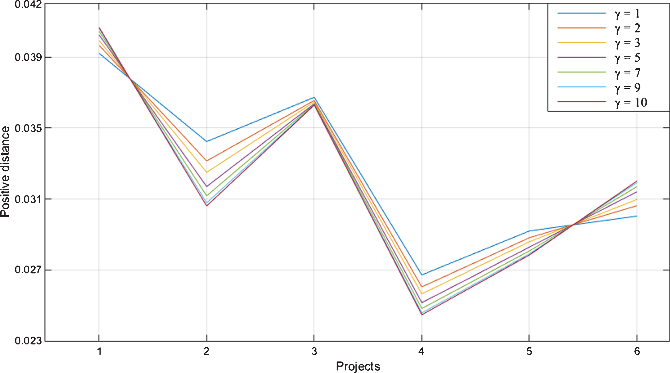
The positive distances of each project with different values of γ.
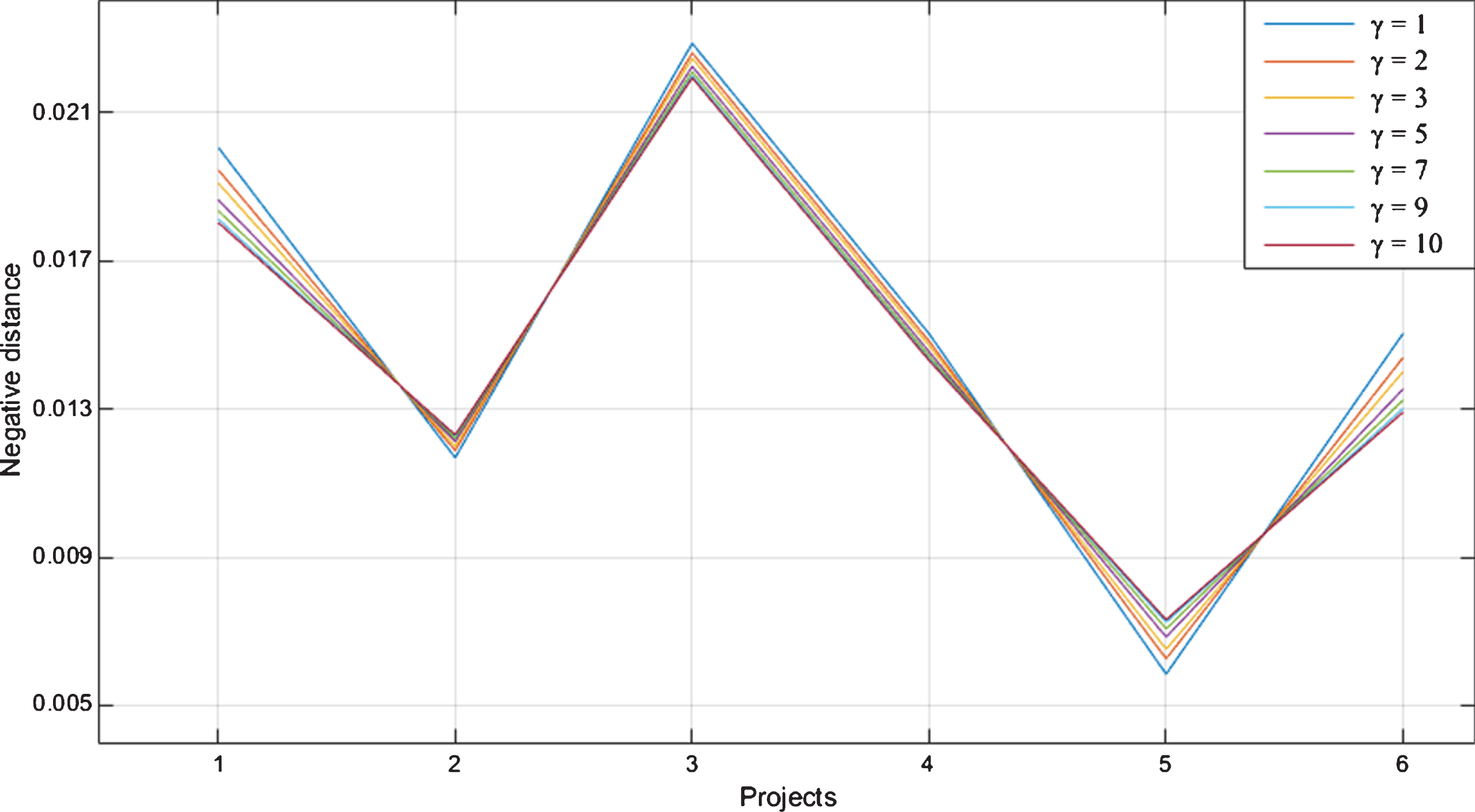
The negative distances of each project with different values of γ.

The positive prospect values of each project with different values of γ.

The negative prospect values of each project with different values of γ.
Form Figs. 8 to 11, it can be concluded that: Our proposed entropy-weighted method has sufficient stability under different values of γ. In each figure, we can see that the shapes of lines are highly similar even if γ changes. However, it does not mean that the role of γ is insignificant. For instance, in Fig. 8, the positive distance of project A2 is greater than that of A6 when γ = 1, and when γ = 10, the relation reverses. In Figs. 8 and 11, with the increase of γ, the positive distances and positive prospect values of A1 and A6 increase, while in Figs. 9 and 11, with the increase of γ, the negative distances and negative prospect values of A1 and A6 decrease. It points out that A1 and A6 benefit from the increase of γ. Nevertheless, it is not always the case for other criteria, such as A2 and A5, which suffer the contrary treatment. In other words, the change of γ may amplify the differences between the projects.
Figs. 8 and 10 are highly similar and so are Figs. 9 and 11. These stress that the positive prospect value keeps consistent with the positive distance, and the negative prospect value keeps consistent with the negative distance, which conforms to the definition of prospect value and shows its practical significance.
To analyze the roles of the irrational degree θ and the risk preference parameter δ in Model (27), different values are taken into the model and obtained the optimal investment ratios. The results are shown in Figs. 12 to 14.

The positive distances of portfolio with different values of the parameters in Model (27).

The negative distances of portfolio with different values of the parameters in Model (27).

The total prospect values of portfolio with different values of the parameters in Model (27).
In according with Figs. 12 to 14, the following conclusions are drawn: The positive distance surface is similar to the negative distance surface, which demonstrates the consistency of return and risk. With the increase of δ, the positive distance and negative distance decrease while the total prospect value increases, which is in line with the analysis in section 5.1. When the value of θ is lower than 0.6, there is little change on the positive distance and negative distance whether θ is changed or not. This means that the portfolio with the optimal solution can afford the investor at least 60% satisfactory degree of prospect value. When θ is higher than 0.6, we can find that with the increase of θ, the positive distance and negative distance decrease intensely because the investor’s sensitivity is higher than rationality. Under this condition, it is difficult for the investor to make rational portfolio selection. Thus, the introduction of the irrational degree θ has great practical significance. To be convenient, we use the rational frontier θ′ to denote the value that satisfies the following conditions: when θ ≤ θ′, the influences of θ on the positive distance and negative distance can be nearly ignored; otherwise, the influences are apparent. Obviously, θ′ is the folding line of the surfaces in the above figures. And then, we can find that θ′ slowly increases while δ increases, which implies that with the increase of the investor’s risk aversion degree, the influence of the irrational degree on Model (27) decreases. In other words, the optimal solution that stands for investment ratios is more stable.
According to the above numerical applications and sensitive analysis, the proposed method has the following advantages: Compared with the conventional entropy-weighted method, the proposed entropy-weighted one can better deal with extreme data and make the allocation of criterion weight more reasonable. In addition, it can effectively reflect decision makers’ confidence degree to the information they hold. In other words, it can avoid the loss of subjective information from decision makers. Instead of average or maximum/minimum, the median is selected as reference point, which can reduce the interference of extreme data as far as possible. And then, by using the distance measure, we can directly describe the deviation between two IFSs to calculate the prospect value without losing the fuzzy information caused by the transformation of IFS to real number. The proposed model can allocate investment ratios without historical data. On the other hand, the prospect value constraint can capture investors’ degree of rationality and then provide a portfolio strategy that meets their preference. If the parameter θ equals to 0, the constraint will be invalid and the proposed model is essentially the same as the traditional M-V model.
Conclusion
In this paper, the portfolio selection problem under intuitionistic fuzzy circumstances is viewed as a kind of multi-criteria decision making (MCDM) problem. Considering that it is unrealistic to require the decision maker to keep completely rational in the decision making process, the prospect theory is utilized to describe the decision maker’s psychological state. Since weight of criterion stands for the decision maker’s subjective preference rather than something objectively existing, it is unreasonable to distort weight by the weighting function. To avoid this problem, we present a new entropy-weighted method with confidence degree. Compared with the conventional entropy-weighted method, our method can not only better deal with extreme data, but also effectively reflect decision makers’ confidence degree to the information they hold.
In addition, we choose the median instead of average or maximum/minimum as reference point, which can reduce the interference of extreme data as far as possible. And then, based on the distance measure, the intuitionistic fuzzy prospect value function is proposed to calculate the prospect value under intuitionistic fuzzy circumstances. In order to analyze the relationship between the prospect value and distance measure, the positive prospect value and negative prospect value are defined. After that, a portfolio selection model with prospect value constraint is constructed to allocate investment ratios. This model adopts the positive distance and negative distance as the measure of return and risk, and introduces the investor’s risk preference. The advantages of the proposed model are that it cannot only allocated investment ratios without historical data, but also flexibly reflect the investor’s degree of rationality by the parameter presented in the prospect value constraint. To illustrate the effectiveness of the model, two numerical applications are given and the sensitive analysis is carried out. The results point out that our proposed model is practical and flexible.
In future work, we will study the combination of prospect theory and multi-objective portfolio selection programming under other kinds of fuzzy circumstances, and then research for an improved algorithm to solve the model more effectively.
Footnotes
Acknowledgment
This research was supported by the “Humanities and Social Sciences Research and Planning Fund of the Ministry of Education of China, No. 18YJAZH014-x2lxY9180090”, “Natural Science Foundation of Guangdong Province, No. 2019A1515011038”, “Soft Science of Guangdong Province, No. 2018A070712002, 2019A101002118” and “Guangdong Graduate Education Innovation Program, 2019SFKC07”. The authors are highly grateful to the referees and editor in-chief for their very helpful comments.