S-CCCapsule: Pneumonia detection in chest X-ray images using skip-connected convolutions and capsule neural network

Abstract

The squash function in capsule networks (CapsNets) dynamic routing is less capable of performing discrimination of non-informative capsules which leads to abnormal activation value distribution of capsules. In this paper, we propose vertical squash (VSquash) to improve the original squash by preventing the activation values of capsules in the primary capsule layer to shrink non-informative capsules, promote discriminative capsules and avoid high information sensitivity. Furthermore, a new neural network, (i) skip-connected convolutional capsule (S-CCCapsule), (ii) Integrated skip-connected convolutional capsules (ISCC) and (iii) Ensemble skip-connected convolutional capsules (ESCC) based on CapsNets are presented where the VSquash is applied in the dynamic routing. In order to achieve uniform distribution of coupling coefficient of probabilities between capsules, we use the Sigmoid function rather than Softmax function. Experiments on Guangzhou Women and Children’s Medical Center (GWCMC), Radiological Society of North America (RSNA) and Mendeley CXR Pneumonia datasets were performed to validate the effectiveness of our proposed methods. We found that our proposed methods produce better accuracy compared to other methods based on model evaluation metrics such as confusion matrix, sensitivity, specificity and Area under the curve (AUC). Our method for pneumonia detection performs better than practicing radiologists. It minimizes human error and reduces diagnosis time.

Keywords

Artificial intelligence capsule network convolutional neural network deep learning pneumonia x-ray imaging

1 Introduction

Pneumonia has increased significantly in global mortality and morbidity in these recent years. In United States, emergency departments [1] accounted for over 500,000 visits and more than 50,000 deaths during the year 2015; which put the diseases among the top 10 causes of the death in the country [2]. Detecting pneumonia early can reduce morbidity and mortality rate and increase the life span of patients. Research conducted by WHO, 2001, revealed Chest X-Rays (CXR) as the current appropriate approach for the diagnosing and detection of pneumonia infection, which in addition plays a crucial part in clinical care and study of epidemiology [3, 4]. However, the detection and diagnosing pneumonia using Chest X-Rays is a challenging task that relies heavily on expert radiologists. The use of human experts for pneumonia detection can be expensive, error-prone and time-consuming. Novice radiologists - especially those working at the rural areas where the quality of healthcare is relatively low - find it hard to diagnose medical imaging. On the other hand, experienced radiologists find it tedious to read hundreds of radiology images per day, as it takes a large chunk of their working time. Overall, both expert and inexperienced radiologists put in a lot of effort to diagnose CXR images. This has motivated the adoption of computer-aided system (CAS) to improve and produce efficient results in pneumonia detection in particular and medical imaging in general. Deep learning (DL) models have achieved impressive performance in recent studies such as method for software maintainability metric prediction [5], assessment of code smell for predicting class change proneness using machine learning [6] and detecting malware using recurrent neural network [7]. Furthermore, DL has recently played an important role in improving the automatic analysis and clinical diagnosis of medical images. Convolutional neural networks (CNNs) methods have been successfully used to perform classification of diseases on medical images. The progress in CNNs have benefited several trials in medical image analysis, such as disease classification [1 , 8–10], image annotation [15, 16], lesion segmentation or detection [14 –18], regression [19], noise induction [20], registration [21] and decision making model based on neutrosophic set for heart disease diagnosis [22]. Rajpurkar et al. [17] developed a CNN model for thorax disease classification. The model inputs CXR images and outputs 14 pathological probabilities, which include the prediction of pneumonia. Although, the model achieved good results on some chest diseases in general, pneumonia in particular achieved low classification performance. Sedai et al. [23] proposed a model that consisted of weak supervised learning and CNN to locate the region of diseases in the CXR images. Their method used disease category labels to avoid the difficulty of obtaining pixel level annotation. However, this approach achieved an unsatisfactory detection accuracy that needs further improvement. Several works on pneumonia classification typically employ CNNs. For instance, Wang et al. [15] evaluated four CNN architectures, such as, AlexNet [24, 25], VGGNet [26], GoogLeNet [27] and ResNet [28], which show the existence of multiple pathologies with global CXR images. To view the CXR detection and classification as a multi-label recognition problem, Yao et al. [29] explored the correlation among the 14 pathological labels using the global images based on the ChestX-ray14 [15]. Using a variant of the DenseNet [30] as an image encoder, the study adopted Long-short Term Memory Networks (LSTM) [31] to capture the dependencies. Kumar et al. [10] investigated the loss function which is more suitable for training CNNs from scratch and presented a boosted cascaded CNN method for global image classification. The recently developed method consists in CheXNet [17]. The method fine-tunes a 121-layer DenseNet on the global CXR images and has a modified fully connected layer. CNNs have greatly achieved promising results in the medical imaging diagnosis. However, CNNs have several issues that reduce accuracy during training. Firstly, CNNs require large amounts of datasets for accurate training and prediction, which in medical imaging are relatively small. Secondly, the pooling layer in CNNs increasingly reduce the resolution of feature maps, thereby causing low accuracy of the network. To account for these issues, Sabour et. al, 2017 proposed dynamic routing between capsules (CapsNet) [29]. They have successfully replaced the pooling layer with a ’dynamic routing agreement’, in which size, color and pose parameters are maintained to improve the network performance. For the CapsNet, the existence of an entity in an image can be depicted by the activity instantiation vector from a collection of neurons. Furthermore, CapsNets can accommodate small datasets for training, which is a great tool for medical imaging especially pneumonia CXR imaging. However, the transformation of the logits by the CapsNet Softmax function into a set of concentrative values may mistakenly transfer the background information from the lower layer to the next layer above, which can lead to wrong summation of the prediction vector with larger values and affect the classification result [32]. The issues with pneumonia diagnosis and CNNs mentioned above motivated us in this study to present a method for detecting whether a patient has pneumonia in CXR images using the prowess of CapsNet algorithm. First, we implemented a CapsNet model, which consists of several skip connected convolution blocks and two primary capsules named skip-connected convolutional capsules (S-CCC) and instead of Softmax for coupling coefficient, we adopted sigmoid function. The intuition for skip connection is to improve the network accuracy, where the input is concatenated with each output of the higher-level convolutions. Second, we implemented integrated skip convolutions with capsules (ISCC), and an ensemble skip connected capsules (ESCC) model with its variant by combining several layer blocks of dense convolutions with CapsNet. Due to constant decreasing of resolutions by the pooling layer, which could cause lower accuracy, the skip connection (performing a dot product with the input layer to each output of the higher level convolutions) was done to account for the loss of information during down-sampling of the pooling.

The contributions of this paper are summarized as follows,

We implemented three architectures: skip-connected convolutional capsule (S-CCCapsule), integrated skip-connected convolutional capsules (ISCC), and ensemble skip-connected convolutional capsules (ESCC), for the pneumonia detection task. The skip-connected property combines the input feature vectors to the higher output convolutions to maintain important information to improve the detection of pneumonia. ISCC and ESCC, and its variants combine the traditional dense max-pool convolution with capsules.

Inspired by [29], we proposed a new routing algorithm. Instead of the conventional squash function, we used vertical squash (VSquash) function. we found that the coupling coefficients based on Softmax function were mainly distributed within smaller interval, which is not well distributed compared to the Sigmoid function. We used the Sigmoid function to assign larger coupling coefficients to real features, while assigning smaller coupling coefficients to the fallacious ones.

We performed extensive experiments on three publicly used datasets, i.e. Guangzhou Women and Children’s Medical Center (GWCMC), RSNA and Mendeley CXR. The experiment results show that the effectiveness of our proposed methods achieve promising performance and significantly outperformed the other baseline methods.

The rest of this paper is organized as follows: Section 2 presents the related works. Section 3 describes problem formulation, background for CNNs, our proposed architecture and CapsNet, followed by experimental details in Section 4, result and discussion in Section 5, Finally, Section 6 concludes the paper.

2 Related works

The goal of Wang et. al. [12] was to initiate future efforts by promoting public databases. The work presented a “machine-human annotated” CXR database that gives a real clinical and methodological challenge of handling tens of thousands of patients. As part of this, they also conducted extensive experiments on the quantitative performance bench marking on eight common thoracic pathology classification and weakly-supervised localization based ChestX-ray 8 database. They implemented multi-labeled CNN architecture with the Caffe framework [25]. The ImageNet pre-trained models, such as AlexNet [24], GoogLeNet [27], VGGNet-16 [26] and ResNet-50 [34] were used from the Caffe model zoo. The integrated DCNN, used weights from the models, transition layers and prediction layers were trained from scratch. Rajpurkar et al. [11] proposed an algorithm that detects pneumonia from frontal-view CXR images at a level to exceed the performance of radiologist. They trained their algorithm using ChestX-ray14 on Dense Convolutional Network (DenseNet) consisting 121-layer [30]. Based on the ability of DenseNets to improve flow of information gradient in the network and make optimization of very deep networks to be tractable, they replaced the final fully connected layer with a layer that has single output and applied sigmoid nonlinearity. Yao et al. [29] presented and evaluated a partial solution to the constraints in adopting LSTMs to overcome interdependency with target labels in predicting 14 pathologic patterns from chest x-rays. They considered the medical issues at hand and proposed a model based on DenseNets [26]. In the first stage, their model inputs were of much higher resolutions. They noted that lower resolution, typically 256 × 256, is enough when solving problems related to natural images, photos and videos while higher resolution is often important to represent regions within images that are small and localized. The size of their presented model was smaller in network depth. Kumar et al. [10] implemented a cascaded network to improve the performance of deep learning model. The method was performed along with modeling label dependencies which is based on the possibility of training Deep Convolutional Neural Network (DCNN) for Computer Aided Diagnosis systems (CADs). In their work, they experimented on a set of deep learning models and proposed a cascaded deep neural network that can diagnose all 14 pathologies better than the baseline and other related published methods. DenseNet161 [3] was used as a baseline neural network architecture, because of its known performance on a variety of datasets. Their work was fully motivated by the modeling DenseNet architecture with few numbers of trainable parameters and was able to reduce over-fitting while benefiting from deep architecture. The cascaded network was designed in a way where every succeeding level in the network can receive prediction from all the prior levels as an input. Qingji et al. [35] presented an attention guided convolutional neural network (AG-CNN) to classify thorax disease. The network consisted of two major branches, known as the global and local branch and included a fusion branch. The global and the local branches were implemented as classification networks to predict the existence of pathologies in the x-ray images. Given an x-ray, the global branch was fine-tuned using a global image. Due to the region of interest to train the local branch, they performed cropping on an attended region of the global image which was used to train for classification on the local branch. Deniz et al. [36] proposed a deep learning structure for a classification task. The network was trained with modified CXR images, using multiple steps during the preprocessing. The classification method used CNNs and residual network (ResNet) architecture to predict whether pneumonia was present or not in the CXR images. A new approach based on weighted classifiers were presented in [37], which combine weighted predictions from state-of-the-art deep learning structures such as ResNet18, Xception, InceptionV3, DenseNet121, and MobileNetV3 for pneumonia prediction. Ansh et al., 2020 [38], explore convolutions and utilized the advantage of dynamic routing procedure in CapsNet for pneumonia CXR detection.

In this study, we present a method for classifying pneumonia based on x-ray image. According to the literature, the CNNs used require large amounts of data; however, the data available in medical imaging are few. In addition, the CNNs do not consider the spatial orientation of the input image which decrease the performance of the networks. We therefore highlight capsule network (CapsNets) for the pneumonia classification task. The introduction of a new routing algorithm with a new squashing method, which we named vertical squash (VSquash) and Sigmoid function for effective coupling coefficient distribution can improve the classification of the networks. We note that our method outperforms previous works.

3 Methods

Detecting pneumonia is a binary classification task where inputs are the frontal-view of CXR, which we denote as X and the corresponding outputs are binary label y ∈ 0, 1 that indicates the presence or absence of pneumonia respectively. Given a training sample, the weighted binary cross [57] entropy loss can be optimized using the Equation 1.

$\begin{matrix} H_{p} (q) = - \frac{1}{N} \sum_{i = 1}^{N} y_{i} \cdot \log (p (y_{i})) + (1 - y_{i}) \\ \cdot \log (1 - p (y_{i})) \end{matrix}$ (1) where y is the label and p (y) is the predicted probability of the point number of positive and negative cases for all N points. In other words, for N data points where y_i is the true value given a value of 0 or 1 and p (y) is the Softmax probability for the i ^th data point.

3.1 Convolutional neural networks

Generally, CNNs consist of three properties: Firstly, neurons in higher layer receive inputs from the lower layers which are localized in a closest neighborhood. In this way, layers such as first layer extracts edges, textures and corners while the upper layers extract high dimensional complex features. These extracted features are combined in the next layer which detect higher complex features. Secondly, the concept of shared weight is an important property of CNNs, which indicates that similar feature detector can be applied to the entire input image. Finally, CNNs usually implement sub-sampling techniques in the layers to reduce the size of the input. We can compute the convolution with the discrete operator ∗ by using translation-invariant. The translation-invariant linear operator from $L^{2} (ℤ_{N})$ into $L^{2} (ℤ_{N})$ can be given a representation that gives detail information in the convolution with signal analysis. Let z and f be a signal in $L^{2} (ℤ_{N})$ . Then we define the signal z ∗ f in $L^{2} (ℤ_{N})$ by $(z * f) (q) = \sum_{n = 0}^{N - 1} z (q - n) f (n), q \in ℤ$ (2) where z ∗ f are the convolution of z and f. Let b be a signal in $L^{2} (ℤ_{N})$ . Here we can define the mapping $C_{b} : L^{2} (ℤ_{N}) \to L^{2} (ℤ_{N})$ by $C_{b} z = b * z, z \in L^{2} (ℤ_{ℕ})$ (3)

CNNs are accepted to provide useful results in many research fields due to the beneficial feature and characteristic it carries. In this work, we noted that the convolution layers do not consider the precise location of the features as beneficial. This makes the approach harmful, because there are variations of information for different instances. Furthermore, several drawbacks of the CNNs are listed as follows:

CNNs requires large amounts of dataset for accurate training and prediction. Regards to this characteristic, the network performs poorly when train with small datasets, which is the case with most medical image datasets such as brain MRIs and CXR images [41 , 44].

CNNs given a small amount of translational invariance can lose the actual location of the most active feature detectors [39, 40]. Hence, CNNs progressively reduce the resolution of feature maps through down-sampling. Such loss of resolution limits the classification accuracy of the network [46].

When multi-layer perceptron is used i.e. if all layers are fully connected, the CNNs find it difficult to compute, due to the high dimension of the input image.

Based on the above-mentioned shortcomings, a new architecture called CapsNet was introduced to mitigate the problems and enhance performance of the network. The CapsNet is robust to translation and rotation compared to the CNNs. This network is reviewed in Section 3.3.

3.2 Proposed architecture

3.2.1 Skip-connected convolutional capsule (S-CCCapsule)

The proposed model introduces feature-level augmentations through skip connections that combines deep, coarse and fine, appearance cues from mid-layers. Further, our model performs 2-dimensional (2D) convolutions with capsules modules, which does a coarse-level feature fusion in a structured manner, as depicted in Fig. 1. The residual feature flows alleviate vanishing gradient of deep networks by moving important information from lower layer to the layers above. Even though the shortcut seems like a summation to the traditional CNN connection, it mitigates training and minimize the number parameters [34, 47].

Fig. 1

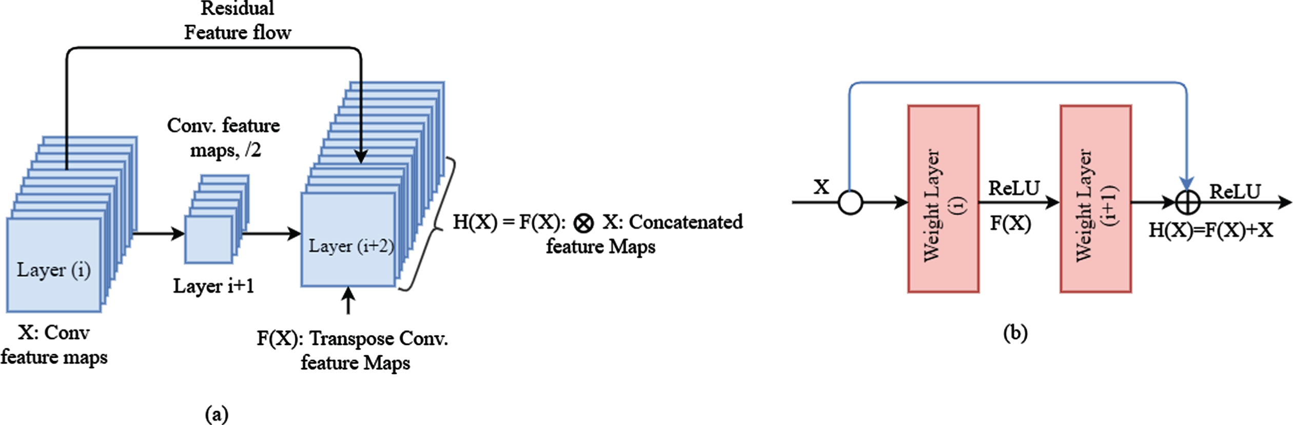
Convolutional feature flow: (a) residual concatenated feature mapping of our proposed models (b) ResNet flow.

An illustration for ResNet connection is shown in Fig. 1(b), where X is an input feature, H (X) is a transformation, and F (X) is a residual mapping. In [35, 47], the operator for feature fusion H (X) = F (X) + X is performed by a short concatenation and element-wise addition. Despite that, our model stacks the features depth-wise as H (X) = F (X) ⊗ X, like in Fig. 1(a), where ⊗ denotes coarse-level feature concatenation. The feature map output of the previous convolution layer and scale are combined using concatenation. That is output of a convolution used on the same-scale feature from the previous convolution layer [43] and output of a strided convolution used on the fine-scale feature vector from the previous convolutional layer computed by concatenating their results. It is favorable to have a smaller number of filters in conv layers resulting less computation.

Figure 2 shows our proposed S-CCCapsule model. The size of the kernel k, stride s, and dimension of the output are described in the following order and in enclosed braces (k, s) [H × W × D] in each layer. Where the H, W and D represent height, width and dimension of the input and feature maps respectively. The entire structure has 9 layers with 8.3M trainable parameters that compose three major components: encoder, decoder and classifier. The encoder is composed of Convolutional layers, primary capsule (PrimaryCaps) layers and disease capsule (DiseaseCaps) layer. In the encoder, we initialized filter size of 96, 64, 32, 32, respectively in the preceding four conv layers where we maintained kernel size, k = 1×1 and stride, s = 1. In contrast, we set the kernel and stride size to 3 and 2 in the two (2) primary capsule layers which produced 21×21 feature maps. The intuition of setting the kernel and stride size to 1 is to achieve high activation map to produce better accuracy. The dynamic routing given in Algorithm 2 is performed between the PrimaryCaps and DiseaseCaps, which this work introduced a vertical squash function (VSquash) to better shrink long vectors to vector slightly close to 1 and short vectors to 0. Instead of Softmax function for distribution of the coupling coefficient, we adopted Sigmoid function which gave better distribution of coupling coefficient. Moreover, the spatial dimension of the feature maps is maintained without striding in the encoding stage except the primary capsule layer where striding the kernel at a rate of 2 are performed. Thus, the PrimaryCaps layer of the encoder generates feature maps that have spatial dimension of 21×21 which is then forward to the last encoder layer called DiseaseCaps. We introduced batch normalization (BN) after conv layers to alleviate over-fitting. To achieve the precise decoded feature maps, there are three fully connected layers which are sequentially connected. The final layer of the decoder network provided output feature maps with same spatial dimension as the input. The fully connected layers consist of dropout rate of 0.2 and 0.5 and finally the last classifier layer consist of sigmoid function as a classifier. For the sake of clarity, we elaborate the concept of capsule network with dynamic routing algorithm which exists between the PrimaryCaps and DiseaseCaps in Section 3.3, Algorithm 2 and Fig. 7.

Fig. 2

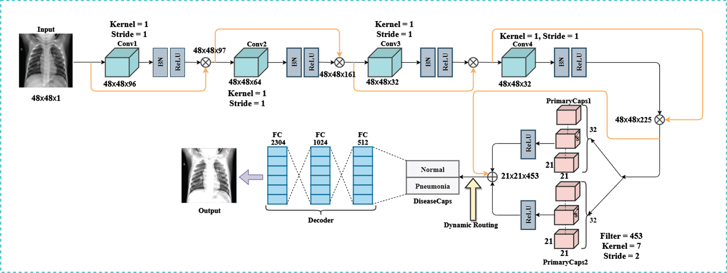
Proposed S-CCCapsules architecture.

Fig. 7

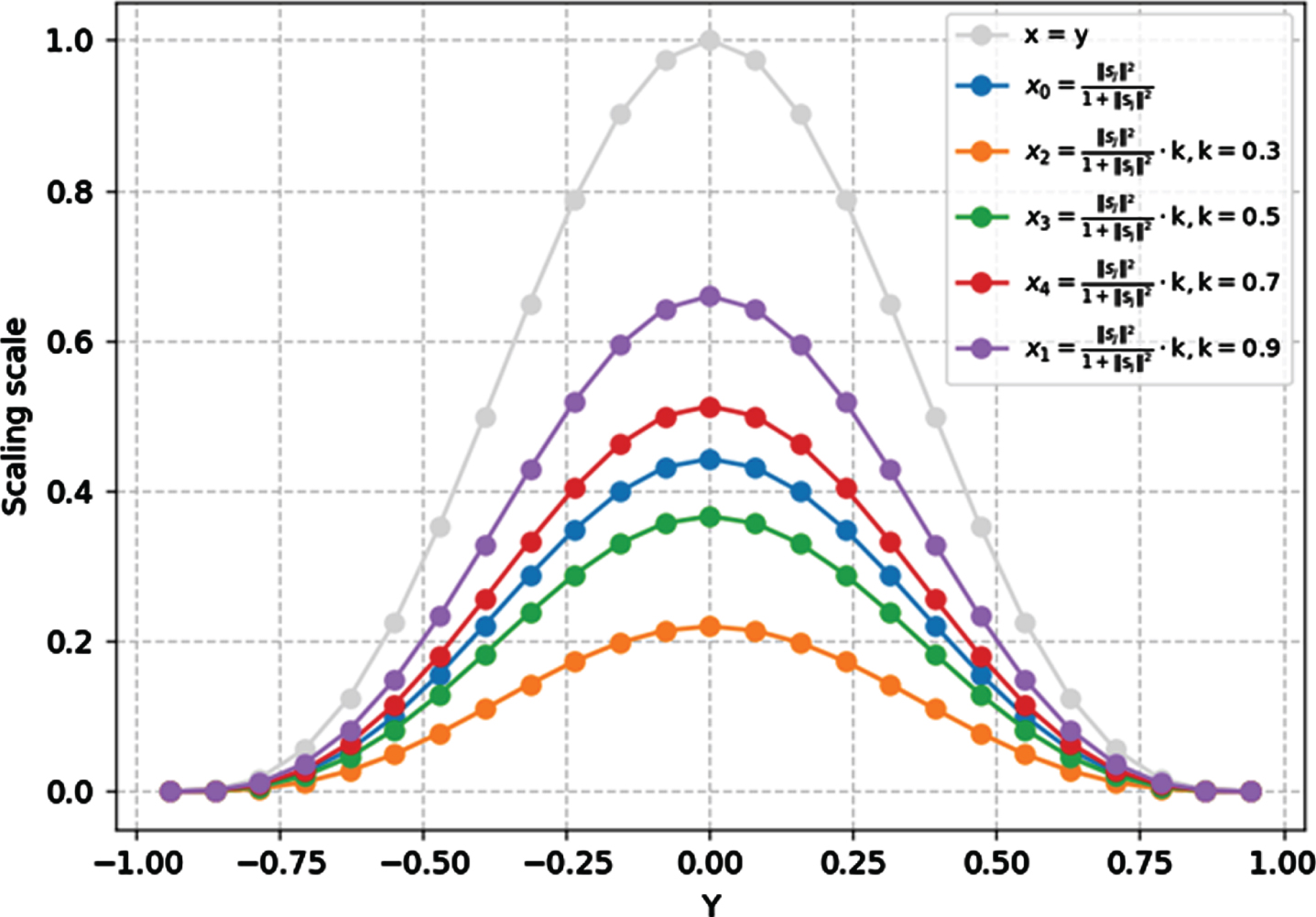
Comparison of different squashing functions.

3.2.2 Integrated skip convolutional capsules (ISCC)

The Integrated skip convolutional capsules (ISCC) shown in Fig. 3 was built for the pneumonia detecting task. The model shows a combination of traditional dense convolutions with capsule layers. The bottom of the model shows a simple capsule block where dynamic routing between PrimaryCaps and PneumoniaCaps are performed. The ISCC network has two main substructures namely, the dense skip convolutional substructure (dSCS) and capsule dynamic routing substructure (CDRS). The substructure dSCS in the ISCC architecture consist of two maxpool layers found in the third and sixth convolution layers. Reference [48] showed that, late down-sampling achieves high activation map, which produce good accuracy. This motivated the introduction of 1×1 kernel size in the dSCS block. In the Conv1 ReLU layer, 32 filter size was used which produced 48×48×32 feature vectors. The Conv2 ReLU layer has 64 filter size that utilizes 48×48×64 and repeated in the Conv3 ReLU followed by maxpool2d_1 with 2×2 kernel size producing 24×24×64 feature vectors. The 4th, 5th, 6th convolutions have the 24×24×128, 24×24×256 and 24×24×512 feature vectors respectively and followed by Maxpool2d_2 of 12×12×512 feature vectors. The bottom layer block CDRS consist of simple capsule model. The Conv7 ReLU of the CDRS gives a dimension of 12×12 feature vectors. The resulting feature vectors from Conv7 ReLU is mapped to the PrimaryCaps layers which has 16 channels of 8-Dimensional capsules. Here every primary capsule produces 8 units, with 3×3 kernels and 2 strides. Each primary capsule is provided with 128×128 from the Conv7 ReLU layer. Hence, the PrimaryCaps produce 5×5×16 feature vectors as output. The capsule 5×5 feature map shares their weight for equivariance with the high-level capsule with the high agreement.

Fig. 3

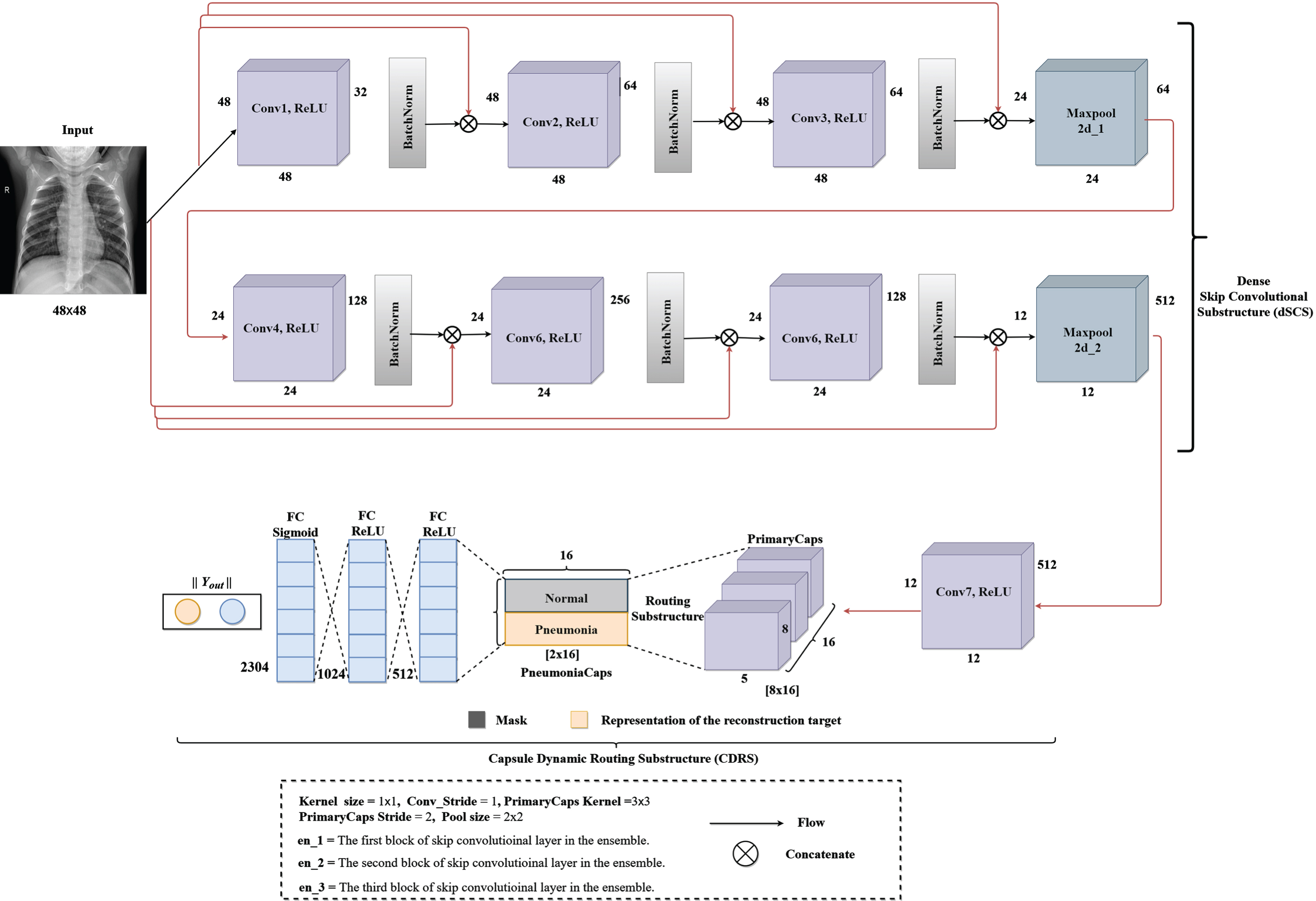
An integrated skip convolution with capsules which we named integrated skip convolutional capsules (ISCC).

We implemented the CDRS substructure with the configuration of the capsule layer (i.e. routing, margin loss etc.). Lastly, Y_out was used to determine the probability “Normal” or “Pneumonia” existing in the CXR image.

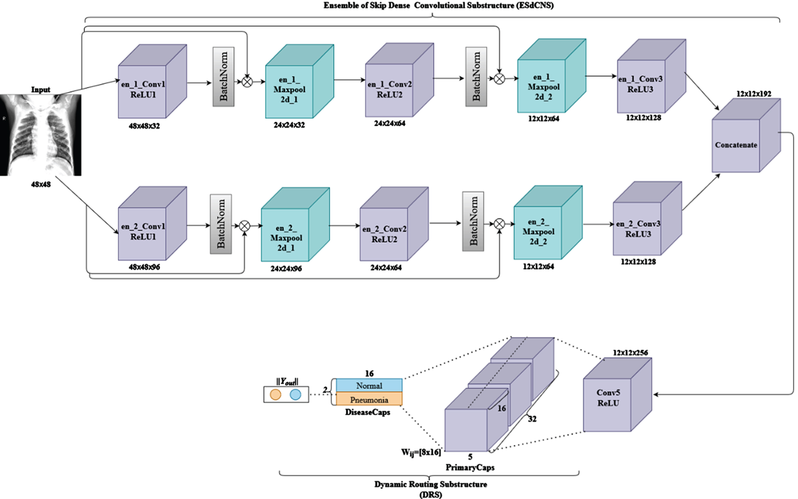
3.2.3 Ensemble of skip convolutional capsules (ESCC)

This model named Ensemble of skipped convolutional capsule (ESCC) presented in Fig. 4 consists of an ensemble of skip convolutions. In addition, the network has substructures namely ensemble skip dense convolution substructure (ESdCNS) and dynamic routing substructure (CDRS). The ESdCNS model consists of 6 convolutions with 4 maxpool layers corresponding to the two divided ensemble convolutions with 2 maxpooling each. The convolutions adopt configuration from the ISCC structure which is kernel size, pool size and nonlinearity function. The en_1_Conv1 layers as the first convolutional layer has 32 feature maps and has 48×48 feature vectors from the input images where maxpooling application is performed to achieve 24×24 feature vectors. BatchNormalization (en_1_Bn_1) is applied after the layers in order to minimize overfitting (as described in the Section 3.2.2). The layers above en_1_Conv consist of 32, 64 and 128 feature maps respectively. The model combines these layers into a single block layer as depicted in ISCC model. We constantly repeated the process through Convolutional layers with ReLU and Max_pool2d layers (i.e. en_1_Conv2, en_1_ReLU2, en_1_Bn2, en_1_Max_pool2d_2, en_1_Conv3, en_1_ReLU3, en_1_Bn3) to produce vector feature maps of 24×24×32 and 12×12×64 in the 2nd block layer and finally, 12×12×128 feature vectors for en_1_Conv3. The second blocks of convolutions with en_2_Conv1 layer has 96 feature maps producing 48×48×96 feature vectors from the input. This is followed by maxpooling layer to get 24×24 feature vectors and dropout (en_2_dropout_1). As shown in Fig. 4, the convolutional with ReLU, maxpooling and dropout are combined to obtain vector feature maps of 24×24×96 and 12×12×64 (i.e. the 2nd block of convolution, maxpool and dropout), finally the last block of convolution en_2_Conv3 produced 12×12×128 feature vectors. The output from en_1_Conv3 and en_2_Conv3 is concatenated, and output feed to the capsule block.

Fig. 4

An integrated skip convolution with capsules which we named Ensemble of skip convolutional capsules (ISCC). The architecture constantly produced high accuracy compared to CapsNet [45] and the ISCC model shown Fig. 3.

3.2.4 Ensemble of n-Skip convolutional capsule (EnSCC)

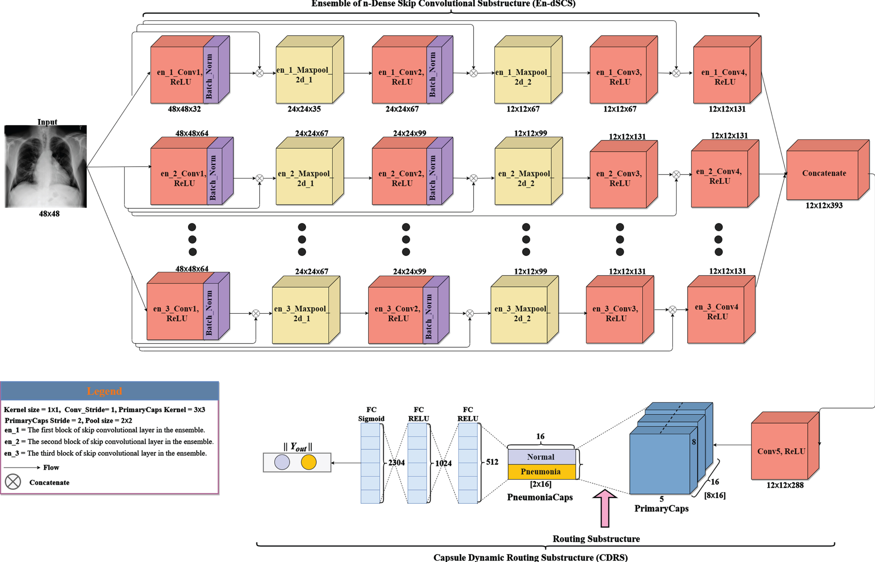
We present a variant of ESCC model which is named Ensemble skip n-convolutional capsule (ESnCCs) shown in Figs. 6. The figures are composed of ensemble skip convolutions like ESCC except for the number of convolutions and primary capsules in the substructure used in these models. These networks have two substructures: the ensemble skip n-dense convolutional substructure (ESnDCS) and dynamic routing substructure (DRS). The number of convolutions is initialized as n, where n ∈ {3, 4, 5, 6, 8}. In the variant ensemble network implemented, the image size used was downscaled from the original size to 48. We present a variant of ESCC model which is named Ensemble skip n-convolutional capsule (ESnCCs) shown in Figs. 6. The figures are composed of ensemble skip convolutions like ESCC except for the number of convolutions and primary capsules in the substructure used in these models. These networks have two substructurescolon the ensemble skip n-dense convolutional substructure (ESnDCS) and dynamic routing substructure (DRS). The number of convolutions is initialized as n, where n ∈ {3, 4, 5, 6, 8}. In the variant ensemble network implemented, the image size used was downscaled from the original size to 48×48 to reduce the number of features and train parameters. The E3SCC model in Fig. 5 is a variant of the ESCC model, which consist of 12 convolutions with 6 maxpooling layers. The 6 maxpooling layers are divided among the ensemble of 3-layer convolutions. The first convolution en_1_Conv1_ReLU layer has 32 feature maps that with 48×48 feature vectors. The feature vector is subjected to a maxpooling to get 24 × 24 feature vectors. In this sub-block, the process is repeated through convolution ReLU layers and Maxpooling layers to get feature maps of vectors 24 × 24 × 67, 12 × 12 × 67, 12 × 12 × 131 (through en_2_Conv2_ReLU, en_1_Maxpoo2d_2, en_3_Conv3_ReLU) and finally, 12×12×131 through en_1_Conv4_ReLU. In the second substructure, the en_2_Conv_ReLU has 64 feature maps that uses 48 × 48 × 64 feature vectors from the input image. The feature vectors are subjected to maxpooling to obtain 24 × 24 × 64 feature vectors. The process is repeated through en_2_Conv2_ReLU, en_2_Maxpool_2d_2, en_2_Conv3_ReLU and finally, en_2_Conv4_ReLU to obtain 24 × 24 × 67, 12 × 12 × 67, 12 × 12 × 131, and 12 × 12 × 131 feature vectors. The third substructure (en_3) operates similarly to the 2nd substructure. In order to regularize the models and minimize overfitting, batch normalization was used after convolutions. Regularization methods and activation functions used are explained in Appendix A and B, respectively.

Fig. 5

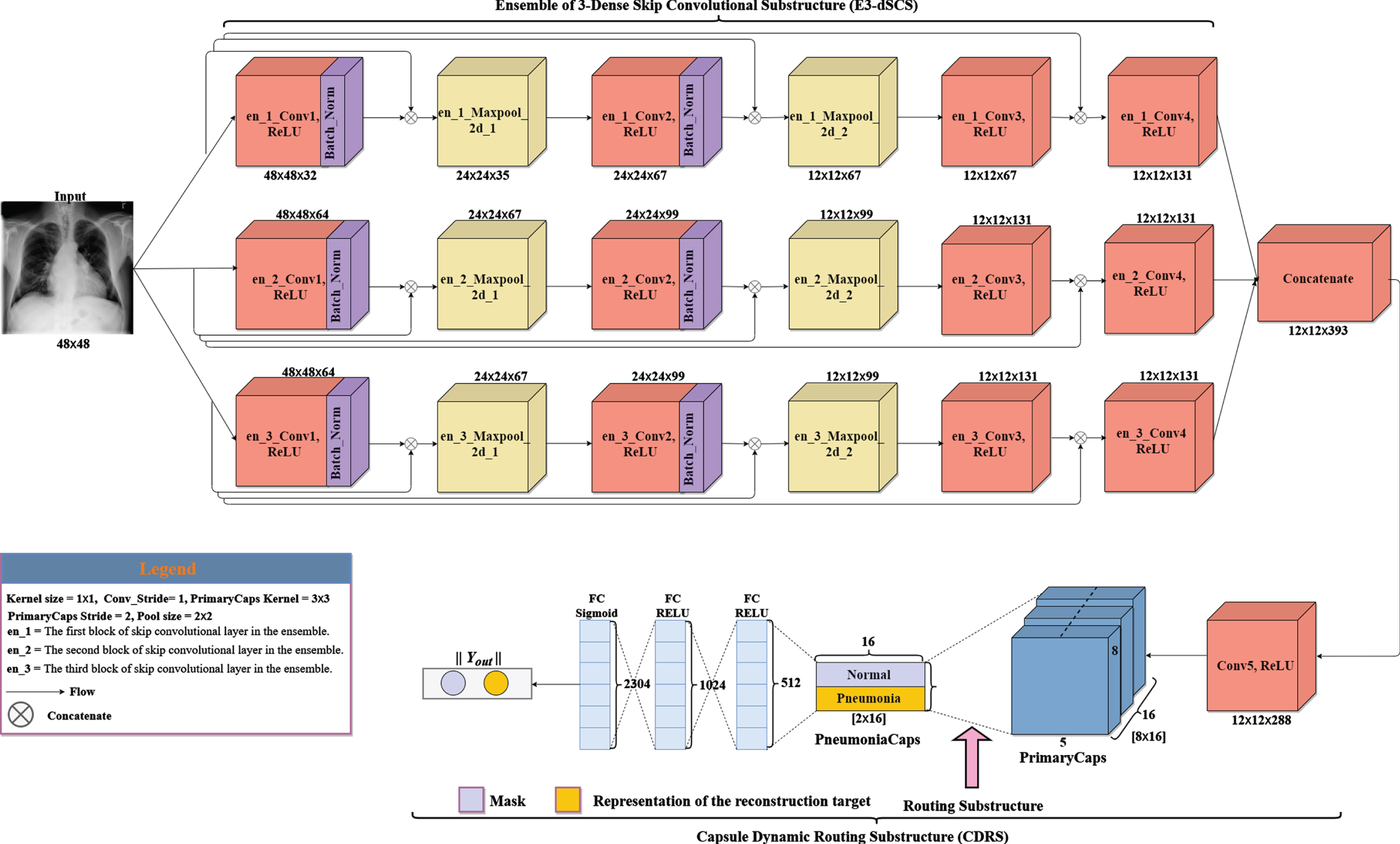
Ensemble of 3-skip convolutions with capsules (E3SCC).

Fig. 6

An Ensemble of n-skip convolutions with capsules (EnSCC) architecture with a decoder layer as a variant of EnSCC.

3.3 Capsule network

The concept of capsule proposed by [42] is defined as the collective neurons indicating activity vectors of the neurons which represent the existing pose parameter. The length of the various vector shows the probability existence of a specific entity. The pooling layer in CNNs mostly pose a challenge to the structure by reducing resolution [49]. With this as a result, CapsNet has successfully substitute pooling layer with routing by agreement method. The “routing by agreement” by CapsNet has shown appropriate replacement of the pooling layer. Based on these criteria, outputs from the lower layer are forward to each parent capsules within the high layers; however, each of their coupling coefficients tend to be different. Every Capsule in the lower layer predicts the output of the parent capsules. When the predictions match with output of the parent capsule, the coupling coefficient for these two capsules are increased. Let q_i be the output of capsule i, its prediction for parent capsule j is computed as ${\hat{q}}_{j | i} = W_{ij} q_{i}$ (4) where in (equation 4) indicates the prediction vector of capsule j ^th output in the higher layer computed by capsule i in the lower layer. The weighting matrix defined as W_ij learns in backwards pass. The result is achieved base on the conformation existing between lower capsules and parent capsule. In addition, coupling coefficients is defined as c_ij and computed using the softmax function below $c_{ij} = \frac{exp (d_{ij})}{\sum_{k} exp (ik)}$ (5) where d_ij indicates the log probability and shows whether capsule i is coupled with capsule j, which is initialized to at the initial stage of the routing by agreement process. Based on this, input vector to the parent capsule j is calculated as $h_{j} = \sum_{i} c_{ij} {\hat{q}}_{j | i}$ (6)

Finally, at this stage, non-linearity squashing function is applied to ensure the output vectors of capsules do not exceed 1 and forms the output of every capsule based on the given value of the initial vector defined in above equation $v_{j} = \frac{| | h_{j} | |^{2}}{1 + | | h_{j} | |^{2}} \frac{h j}{| | h_{j}}$ (7) where h_j is the input vector to capsule while v_j is the output. CapsNets apply the non-linearity squashing function on output vectors v_j for every iteration [50]. It bounds to the likelihood of the vectors between 0 and 1, which means that the squash function suppresses each small vector and maintains the long vectors in unit length. ${\begin{matrix} v_{j} \approx | | h_{j} | | h_{j} = 0, & if h_{j} is small \\ v_{j} \approx \frac{| | h_{j} | |}{| | h_{j} | |}, & otherwise \end{matrix}$ (8)

The log probabilities are updated in the routing process based on the agreement between v_j and using the fact that if the two vectors agree, their inner product will be large. Therefore, agreement for updating log probabilities and the coupling coefficients can be computed as $a_{ij} = v_{j} {\hat{q}}_{j | i}$ (9)

Each capsule n in the last layer is a match to the loss function l_n, which puts high loss on capsules that have long output instantiation parameters when entity does not exist. The loss function l_n is calculated as $\begin{matrix} l_{k} = P_{n} \max (0, z^{+} - | | v_{n} | |)^{2} + λ (1 - P_{n}) \\ \max (0, | | v_{n} | |, - z^{-})^{2} \end{matrix}$ (10) where P_n is 1 whenever the class n is present, and is 0 otherwise. The hyper parameters to be initialized for training process are the terms z ⁺, z ^- and λ. The baseline capsule network architecture consists of 1-layer convolutional network, capsule layers and 3 fully connected networks which perform reconstruction on inputs by using the instantiation parameters from capsules associated with the true labels. Algorithm 1 summarizes the concept of CapsNet dynamic routing procedure.

In this paper, instead of Softmax function (Equation 5) for coupling coefficient in Algorithm 1, we adopted Sigmoid function (Equation 11) to scale the transforming space and calculated the coefficient to enhance the capsule. $c_{ij} = \frac{1}{1 + exp (b_{ij})}$ (11)

Routing using the Sigmoid is same as the Softmax routing procedure in [33], but we rather used Sigmoid function as shown in Equation (11). Here the c_ij does not mean the allocation of probabilities toward the final capsules in reference [28], but represents the strength of correlation between the primary capsules and the final capsules. Replacing Softmax function with Sigmoid function for coupling coefficient gives more improvements to the capsule, such as: 1. The important predictor vectors are multiplied by large coupling coefficients, which makes the significant feature more decisive, while unrelated figures get smaller ones. Additionally, it increases the difference between the lengths of the vectors in the final capsule layer, where the correct digit capsule exceeds all the other digit capsules in length. The adoption of the Sigmoid function in our models produced better performance compared to using Softmax routing. In summary, this work modified Algorithm 1 by replacing the Softmax function and squash function with Sigmoid function and VSquash function, respectively, to obtain Algorithm 2. The Algorithm 1 shows the Softmax function with original squash function while our Algorithm 2 shows the Sigmoid function routing with VSquash function procedure.

Algorithm 1 Softmax Routing Procedure by (Sabour et al . , 2017) (CapsNet)

1: procedure Input to Routing Procedure:(j|i, r, l) ⊳ This is a test

2: for capsule i in layer l and capsule j in layer (l + 1) : (b_ij ← 0)

3: for r iterations: do

4: for capsule i in layer l: c_ij ← Softmax (b_ij) ⊳ softmax computes Equation 5

5: for capsule j in layer (l + 1) : $s_{j} \leftarrow \sum_{i} c_{ij} {\hat{u}}_{j | i}$

6: for capsule j in layer (l + 1) : v_j ← Squash (s_j) ⊳ squash computes Equation 7

7: for capsule i in layer l and capsule j in layer (l + 1) : $b_{ij} \leftarrow + {\hat{u}}_{j | i} \cdot v_{j}$

8: Return v_j

Algorithm 2 Sigmoid Routing Procedure with VSquash (Adu et al . ,) (S - CCCapsule)

1: procedure Input to Routing Procedure:(j|i, r, l) ⊳ This is a test

2: for capsule i in layer l and capsule j in layer (l + 1) : (b_ij ← 0)

3: for r iterations: do

4: for capsule i in layer l: c_ij ← Softmax (b_ij) ⊳ sigmoid computes Equation 11

5: for capsule j in layer (l + 1) : $s_{j} \leftarrow \sum_{i} c_{ij} {\hat{u}}_{j | i}$

6: for capsule j in layer (l + 1) : v_j ← V Squash (s_j) ⊳ VSquash computes Equation 12

7: for capsule i in layer l and capsule j in layer (l + 1) : $b_{ij} \leftarrow + {\hat{u}}_{j | i} \cdot v_{j}$

8: Return v_j

3.4 Vertical squash function

In order to enhance capsule routing, we replace the squash function (Equation 7) with our proposed vertical squash function, which we named VSquash shown in Equation 12. The function is used to restrict the vector h_j close to 1 as shown in Equation 7. The squash function compresses short vectors to a length close 0 and long vectors slightly close 1. Equation 7 is the original squash function represents the scale with $\frac{S_{j}}{| | S_{j} | |}$ indicating the unit vector of S_j. The traditional squash function has less ability to solve higher information sensitivity of capsule networks to distinguish non-informative capsule leading to abnormal activation value distribution of capsules in the primaryCaps layer in [33]. The original squash function generates large activation values for small ||S_j|| that results to faster initial growth of the function. Furthermore, Fig. 7 shows a comparison of original squash (blue) and VSquash over computing initial activation function of primaryCaps. The original squash produces high activation values for capsule with small ||S_j||, which shows how fast they increase from the origin. This shows that the function does not produce better sparsity to constrain capsule from keeping high activation values. $v_{j} = \frac{| | h_{j} | |^{2}}{1 + | | h_{j} | |^{2}} \times k$ (12)

If 0 < k < 1, the vector of function v_j vertically shrunk by multiplying each of the vector h_j by constant figure k. 0 < k < 1. The models with VSquash (i.e. k = 0.5) achieved improved accuracy than the squash function in [33]. In Algorithm 2, we show the improved Sigmoid function routing with VSquash function. Figure 7 shows a comparison of squash function in [33] and VSquash function with different k initializations.

The steps in Algorithm 2 and Fig. 8 are shown as follows:

Set all the probability, parameters and let all b equals to 0 to make C distribute evenly using Softmax as a normalize function.

Convert all input data using the attitude matrix.

Apply dynamic routing to the input weights. Using the formula C_ij U_j|i, update these parameters to make decision about the mapping between the levels. Where C_ij indicates the weight and the sum is equal to 1.

The weight sum gets the average position of features of the object in the image. The output of the Sigmoid function is non-negative and it’s equal to 1.

Use nonlinearity VSquash function as activation in equation 12, where h is united and converted to final vector v, which is the modular length and final output.

Fig. 8

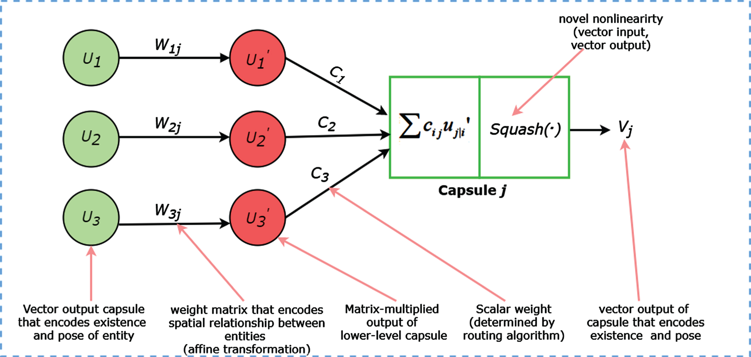
Capsule networks routing algorithm.

4 Experimental details

4.1 Dataset

This section introduces the datasets used to train our model. We used three public datasets (i.e. Guangzhou Women and Children’s Medical Center (GWCMC), Mendeley CXR and Radiological Society of North America (RSNA)). For the GWCMC data, there are 5,863 chest x-ray images and are categories into “Pneumonia” and “Normal”. The data was released by a public website, kaggle.com and are organized into 2 folders (train, test) which contains subfolders for each image category (Pneumonia/Normal). The CXR images were chosen from retrospective cohorts of pediatric patients from one to five years old from (GWCMC), Guangzhou. As part of the patient’s routine clinical care, all the CXR imaging was performed. The chest radiographs were screened, and low quality or unreadable scan removed for quality control. We note that the diagnoses of the images were graded by physicians and approved before training on the AI system. Secondly, we used CXR images taken from the Mendeley CXR dataset [51]. The data consist of 5857 CXR images and divided into 2 classes: “Normal” and “Pneumonia”. Our third dataset for the experiment was released by kaggle.com. The data was provided by the RSNA, which specified the identity of an x-ray image and indicate the presence of pneumonia in the x-ray data. The data contains 29,684 x-ray images. We used 26,684 images for training and 3,000 thousand were used for testing. Table 1 presents the distribution (i.e. classes, training, testing, validation set and total data set) of the used datasets. Samples of the x-ray images are shown in Fig. 9, showing the normal chest x-ray (no infection) and pneumonia chest x-ray (infected with bacteria and virus).

Table 1
Distribution of pneumonia CXR images into training, testing, validation and total set

Dataset Classes Train set Test set Validation set Total Total set

GWCMC Normal 1341 234 8 1583 5865

Pneumonia 3875 390 8 4273

RSNA Normal 1341 234 - 1575 31259

Pneumonia 26684 3000 - 29684

Mendeley CXR Normal 1108 237 238 1593 5857

Pneumonia 2992 641 641 4274

Dataset	Classes	Train set	Test set	Validation set	Total	Total set
GWCMC	Normal	1341	234	8	1583	5865
	Pneumonia	3875	390	8	4273
RSNA	Normal	1341	234	-	1575	31259
	Pneumonia	26684	3000	-	29684
Mendeley CXR	Normal	1108	237	238	1593	5857
	Pneumonia	2992	641	641	4274

Fig. 9

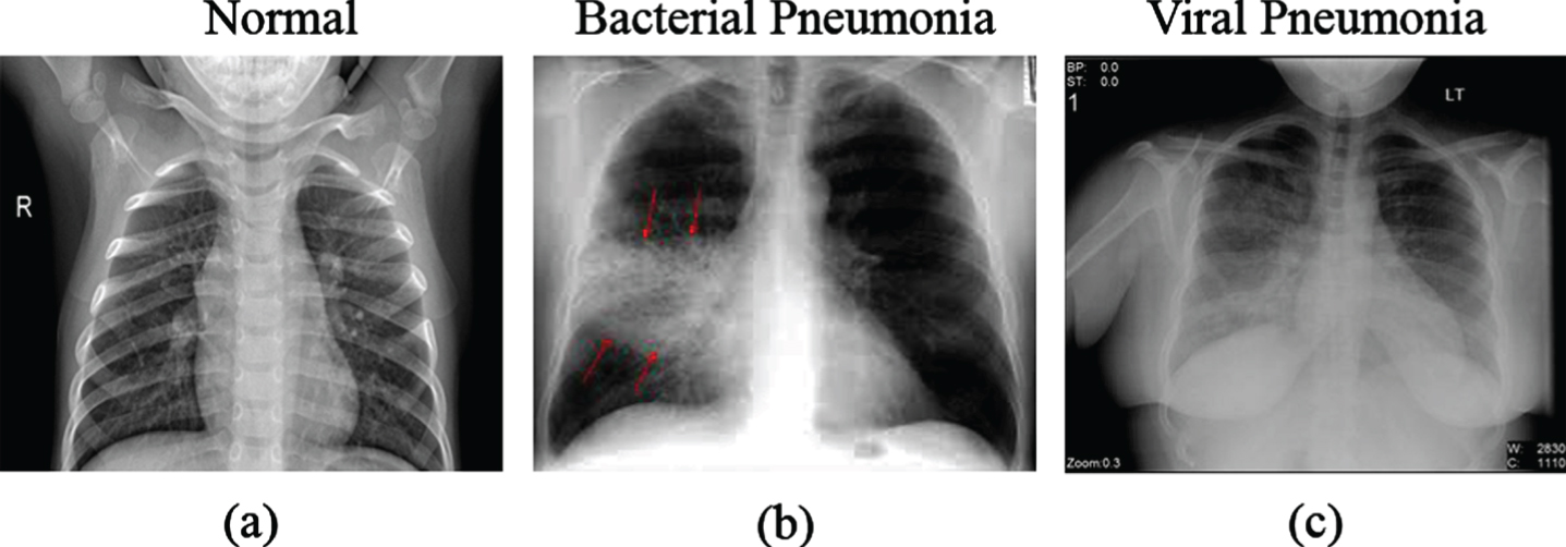
Sample CXR images from patient’s pneumonia diagnosis. (a) shows the normal chest x-ray with clear lungs and without any abnormal opacification within the image. The middle image (b) shows a pneumonia infection by bacterial which is a typical focal lobar consolidation appearing in the right upper lobe with the red arrows. Finally, the last x-ray (c) shows a pneumonia infection by virus manifesting with more diffuse pattern in both lungs.

4.2 Trained networks

Our experiments and evaluations were conducted with Keras deep learning libraries with TensorFlow backend. NVIDIA GeForce GTX 1060 6GB GPU system was used for the experiments. Secondly, the original CapsNet architecture [33] was used for better comparison with the our proposed method.

5 Results and discussion

This section presents the result and discussion of our models experiment. We show the result from our experiments with S-CCCapsule architecture and its three ablation study architectures in Table 2. For our capsule network architecture, we implemented convolutional layers and two (2) capsules in the primary capsule layer. Alongside hyperparameter tuning, we added a dropout layer after every activation to prevent overfitting and sigmoid function at the last FC layer for output. To enable our network with rapid convergence, we used the Adam optimizer which was better than the other optimizers [52]. Binary cross entropy was used as our loss function and sequentially applied dropout rates of 0.4 and 0.6. The dropout function was used randomly to remove a specified number of neurons in the neural network. On the RSNA data, we performed experiments with training epochs of 150 and filter size of 96. Training on the Mendeley CXR pneumonia data, epochs of 300 was used with filter size 96 and batch size set to 32. For the GWCMC data, we trained with filter size of 96. We used batch size of 32, learning rate of 0.0001 and applied ReLU as the transfer function on the three datasets. The use of ReLU transfer provided the network with a good reconstruction compared to the other activation functions.

Table 2
Comparison S-CCCapsules with three different ablation models. The models are compared on basis of validation accuracy, AUC, Precision and Train Time. The best results are indicated in bold

Dataset CapsNet+Maxpooling BSCapsNet LSCapsNet S-CCCapsule

GWCMC 81.89 80.29 79.33 83.65

AUC 0.76 0.74 0.73 0.79

Precision 0.78 0.76 0.75 0.80

Sensitivity 0.98 0.99 0.99 0.98

Specificity 0.94 0.97 0.97 0.95

Train Time 19s 4ms/step 26s 5ms/step 26s 7ms/step 15s 4ms/step

RSNA 96.78 95.52 96.44 99.35

AUC 0.94 0.93 0.92 0.96

Precision 0.94 0.93 0.94 0.99

Sensitivity 0.99 0.99 0.99 1.000

Specificity 0.84 0.75 0.83 1.000

Train Time 57s 15ms/step 160s 9ms/step 287s 12ms/step 326s 12ms/step

Mendeley CXR 88.94 89.74 87.66 91.35

AUC 0.86 0.87 0.84 0.89

Pre_Rec 0.86 0.87 0.84 0.89

Sensitivity 0.98 0.98 0.99 0.97

Specificity 0.95 0.95 0.97 0.95

Train Time 19s 4ms/step 27s 5ms/step 7 107s 20ms/step 62 12ms/step

Parameters 7.8M 5M 12M 8.3M

Dataset	CapsNet+Maxpooling	BSCapsNet	LSCapsNet	S-CCCapsule
GWCMC	81.89	80.29	79.33	83.65
AUC	0.76	0.74	0.73	0.79
Precision	0.78	0.76	0.75	0.80
Sensitivity	0.98	0.99	0.99	0.98
Specificity	0.94	0.97	0.97	0.95
Train Time	19s 4ms/step	26s 5ms/step	26s 7ms/step	15s 4ms/step
RSNA	96.78	95.52	96.44	99.35
AUC	0.94	0.93	0.92	0.96
Precision	0.94	0.93	0.94	0.99
Sensitivity	0.99	0.99	0.99	1.000
Specificity	0.84	0.75	0.83	1.000
Train Time	57s 15ms/step	160s 9ms/step	287s 12ms/step	326s 12ms/step
Mendeley CXR	88.94	89.74	87.66	91.35
AUC	0.86	0.87	0.84	0.89
Pre_Rec	0.86	0.87	0.84	0.89
Sensitivity	0.98	0.98	0.99	0.97
Specificity	0.95	0.95	0.97	0.95
Train Time	19s 4ms/step	27s 5ms/step 7	107s 20ms/step	62 12ms/step
Parameters	7.8M	5M	12M	8.3M

5.1 Classification accuracies

We evaluated and compared S-CCCapsule with four state-of-art method, which used supervised classification methods using the three publicly available chest x-ray datasets. For fair comparison, we evaluated the S-CCCapsule with a baseline CapsNet model. The results in terms of accuracy for all the datasets are provided in Table 2, where the best produced results are marked in bold.

5.2 Ablation study

In [47], an ablation study has shown to be a useful tool for comparative study of models. Therefore, we considered an ablation study for the proposed architecture. Through the study, we resulted in three more architectures namely, CapsNet+Maxpooling, basic simple capsules (BSCapsNet) and long skip capsules (LSCapsNet). To effectively demonstrate the effect of capsule network with dynamic routing, we introduced maxpooling. We conducted experiments on all the datasets with the different ablation architectures. We performed training and testing on the datasets with CapsNet+Maxpooling, BSCapsNet, LSCapsNet and compared the results to our proposed model S-CCCapsule. The ablation results are presented in Table 2, where we can see our proposed architecture outperforms the ablation models in terms of validation accuracy.

CapsNet+Maxpooling: We removed skip connection, used 2 conv layers, 1 primaryCaps and introduced Maxpooling.

BSCapsNet: We removed the skip connection, reduced the convolutional layers to 2 and maintained 2 primaryCaps. We added batch normalization before every ReLU activation to reduce over-fitting.

LSCapsNet: In this model, we used 2 conv layers, introduced long skip connection and reduced the primaryCaps to 1.

The proposed S-CCCapsule architecture has more parameters compared to maxpooling. The intuition is that, maxpooling does not have any parameters to perform feature routing. Whiles in capsules, dynamic routing selects features dynamically and use weights for the features. For any captured important feature, the weight assigned tends to be high. Hence, dynamic routing is better option compared to maxpooling as we gave detail explanation in Section 3.3 above. In Table 2, we can conclude that S-CCCapsule on GWCMC, RSNA and Mendeley CXR images achieves 83.65%, 99.35%and 91.35%, respectively, which are better performances compared to the other three feature extractors in terms of the accuracy. The training accuracy, validation accuracy, loss and confusion matrix of the S - CCCapsule model mentioned in Fig. 2 are given in Fig. 10 as the best training model. For better evaluation of S-CCCapsule, we present the confusion matrix of the three ablation architectures in Fig. 11. We can observe that the Capsule+Maxpooling model Fig. 11(a) produced 7 false negatives (FNs) (1.80%of the “Pneumonia” CXR images) from the CXR validation set 624 images. In diagnosing pneumonia, FNs can be a critical as a patient who has pneumonia may be diagnosed to be healthy and may not be treated. In contrast, the model had 106 false positives (FPs) (45.3%of the “Normal” CXR images), which are normal CXR images diagnosed as pneumonia. The ablation architecture, BSCapsule confusion matrix is given in Fig. 11(b). The model classified 3 instances of the pneumonia as FNs (0.77%of the “Pneumonia” CXR images) and 387 instances positively as pneumonia (99.23%) from the validation set of 624 images. Meanwhile, the model had 120 FPs (51.28%of the “Normal” CXR images), which normal CXR images predicted as pneumonia. The LSCapsule architecture Fig. 11(c) predicted 3 instances of the pneumonia as FNs (0.77%) and 387 instances predicted as true positives (TPs). On the other hand, LSCapsule had 126 FPs (53.85%of the “Normal” CXR image), which is normal patients diagnosed as pneumonia patients. Finally, on the GWCMC images, our proposed architecture S-CCCapsule produced 7 (1.79%) instances of the pneumonia CXR images as FNs and 383 (98.21%) instances of the pneumonia images predicted as actual pneumonia (TPs). The FPs from the S-CCCapsule was 95 instances (50.60%of the “Normal” CXR images). It can be observed from the confusion matrix that, though the number of FNs minimize, but the FPs increased or decreased. The predicted FPs are not harmful compared to FNs, because a person who is not infected by pneumonia, but diagnosed as pneumonia patient would be subjected to treatment. Therefore, the number of FPs is accepted in a certain scope unless the patient is affected by different diseases.

Fig. 10

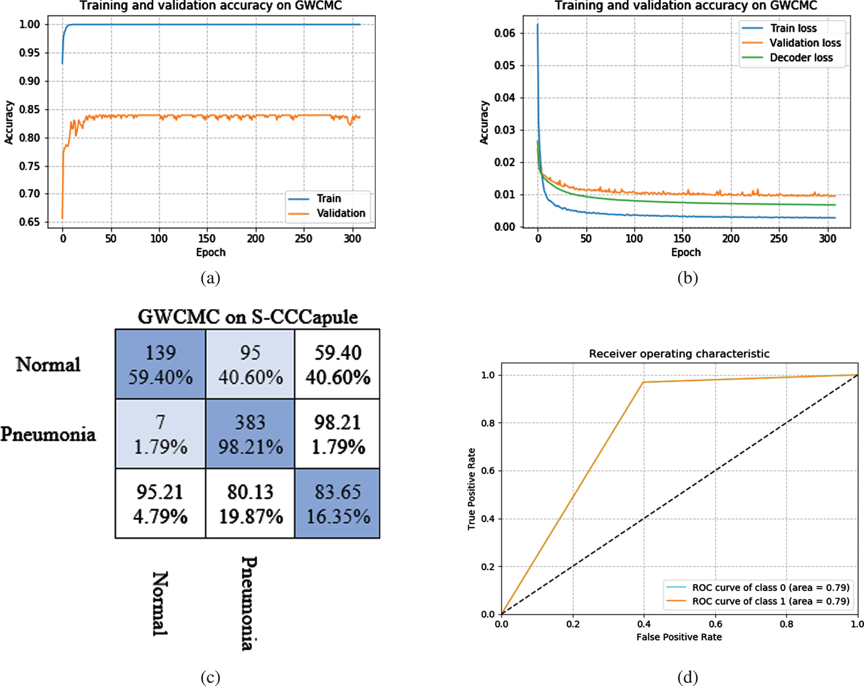
S-CCCapsule training, validation and loss curves on GWCMC images dataset. (a) Training (blue) and Validation (orange color) accuracy curve. (b) Training (blue) and validation (orange color) loss curves, (c) presents the confusion matrix of the 2 classes: “Normal” and “Pneumonia”, and (d) shows the AUC, where S-CCCapsule achieved 0.79.

Fig. 11

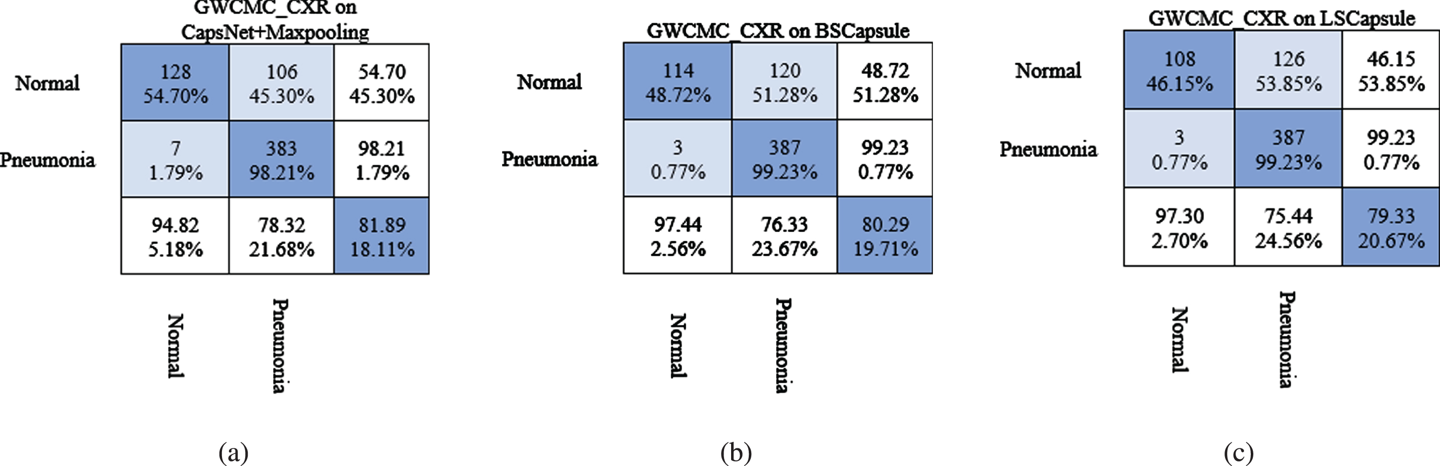
Confusion matrix for Pneumonia detection on GWCMC CXR images using the ablation models. (a) CapsNet+Maxpooling, (b) BSCapsule and (c) LSCapsule.

In Fig. 12, we present the training, validation accuracy (a), train loss, validation loss, decoder loss (b), confusion matrix (c) and area under curve (AUC (d)) of the S-CCCapsule on RSNA CXR images. In training the RSNA CXR images using S-CCCapsule model, we set epoch of 150, meanwhile, the model converged at epoch 64 with 99.35%. The model produced a better probability of discriminating the two class (“Normal” and Pneumonia), with AUC score of 0.96%as presented in Fig. 10(d). In the confusion matrix (Fig. 12(c)), 0 instance was predicted as FNs (0%of the “Pneumonia” CXR images) and 3000 instances (100%) predicted as true pneumonia instances from the CXR validation set 3234 images. On the other hand, 21 instances (8.97%) of the normal images were predicted as pneumonia (FPs) and 213 instances (91.03%) were predicted as true negative (TNs), which is a person with no pneumonia condition predicted to be free from pneumonia. As discussed earlier, the number FPs predicted is not harmful compared to the number FNs, where pneumonia patients are wrongly diagnosed as healthy patients and denied from treatment.

Fig. 12

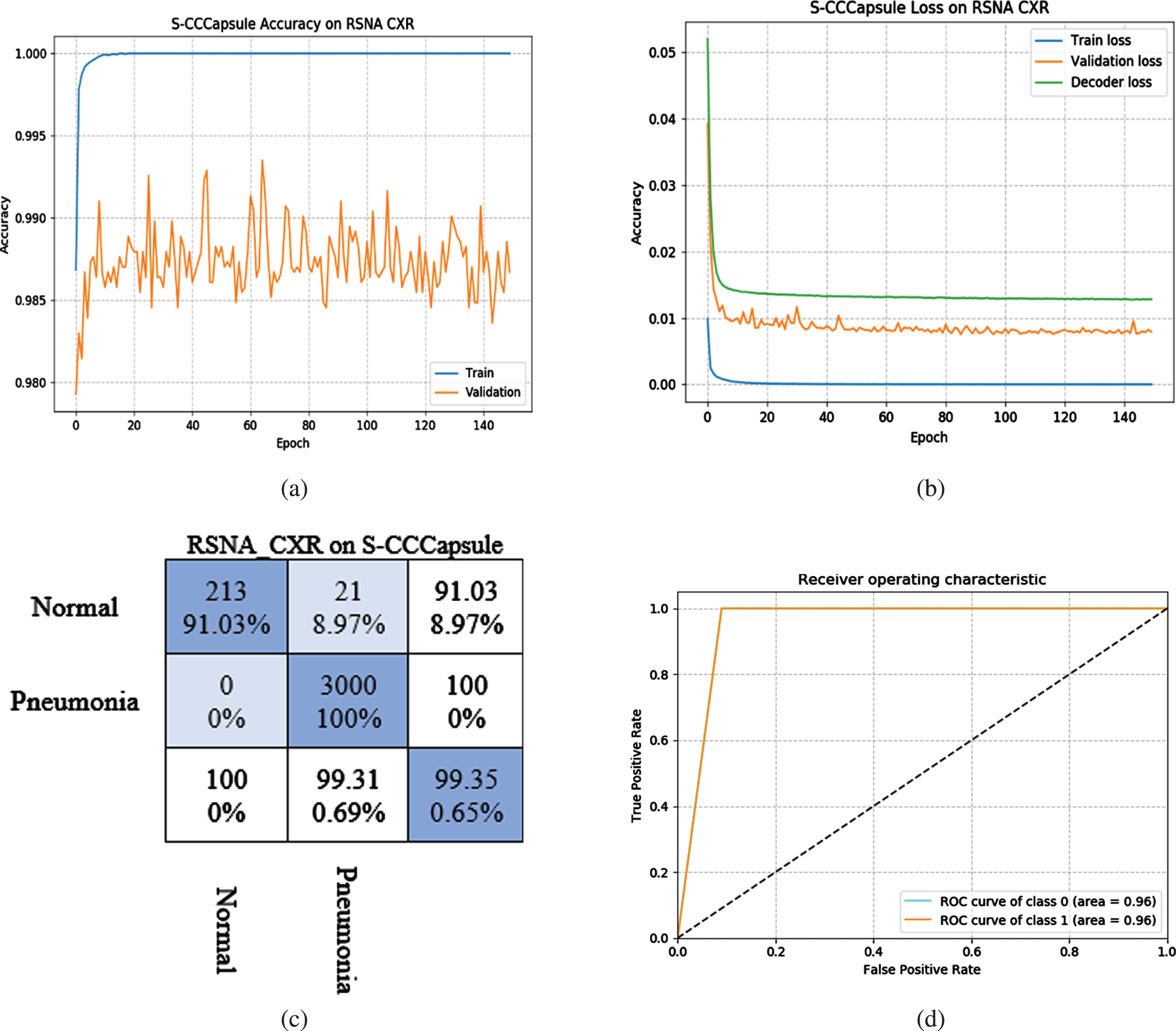
S-CCCapsule training, validation and loss curves on RSNA CXR images dataset. (a) Training (blue) and Validation (orange color) accuracy curve. (b) Training (blue) and validation (orange color) loss curves, (c) presents the confusion matrix of the 2 classes: “Normal” and “Pneumonia”, and (d) shows the AUC, where S-CCCapsule achieved 0.96.

Finally, Fig. 13 presents the training, validation accuracy (a), train loss, validation loss, decoder loss (b), confusion matrix (c) and area under curve (AUC (d)) of the S-CCCapsule on Mendeley CXR images. On the Mendeley CXR images, S-CCCapsule achieved the best result at epoch 15 with 91.35%superior to the ablation models (i.e. CapsNet+Maxpooling, BSCapsNet and LSCapsNet) with 88.94%, 89.74%and 87.10%, respectively. In the confusion matrix (Fig. 13(c)), 10 instances were predicted as FNs (2.56%of the “Pneumonia” CXR images) and 380 instances (97.44%) predicted as true pneumonia instances from the CXR validation set 624 images. On the other hand, 44 instances (18.80%) of the normal images were predicted as pneumonia (FPs) and 190 instances were predicted as TNs (81.20%of the “Normal” CXR images). As discussed earlier, the number FPs predicted is not harmful compared to the number FNs, where pneumonia patients are wrongly diagnosed as healthy patients and denied from treatment. The AUC 0.89%in Fig. 13(d), shows the probability of the S-CCCapsule to efficiently separate the two classes (“Normal” and Pneumonia). Additionally, the S-CCCapsule had precision score of 0.89, which is higher than the other ablation models. Although, the train time per epoch and step was high compared to that of CapsNet+Maxpooling and BSCapsNet, but gained start-of-the-art accuracy due to efficient distribution of coupling coefficient using Sigmoid, effective vector squashing with the proposed VSquash function in the routing algorithm and finally, important information in the images was well aggregated using the skip connection method.

Fig. 13

S-CCCapsule training, validation and loss curves on Mendeley CXR images dataset. (a) Training (blue) and Validation (orange color) accuracy curve. (b) Training (blue) and validation (orange color) loss curves, (c) presents the confusion matrix of the 2 classes: “Normal” and “Pneumonia”, and (d) shows the AUC, where S-CCCapsule achieved 0.89.

5.3 Results on integrated and ensemble architectures

Tables 3 , 4 and 5 represent the training accuracy on GWCMC, RSNA and Mendeley CXR image datasets using the ISCC and ESCC models describe earlier. The figures presented represent CapsNet accuracy, CapsNet loss, Decoder loss and the total loss (the sum of all loses). We note that the name CapsNet accuracy and all other term mentioned have CapsNet, because the architectures have capsule layers.

Table 3
Comparison of models for Pneumonia detection from chest X-Ray images on GWCMC dataset. The comparison was performed based on number of epochs, CapsNet accuracy, CapsNet loss, Decoder loss, total loss, Area Under Curve accuracy and Precision Recall accuracy

Metrics CapsNet ISCC ESCC E3SCC E4SCC E5SCC E6SCC E8SCC

Epochs 170 150 300 300 213 250 160 160

CPN_train 0.9989 1.0000 1.0000 0.9990 1.0000 1.0000 0.9997 1.0000

CPN_val 0.7276 0.8109 0.8465 0.7917 0.8606 0.8478 0.8638 0.8974

CPNLoss_train 0.0045 0.0002 0.0002 0.0020 0.0021 0.0030 0.0121 0.0027

CPNLoss_val 0.2318 0.1477 0.1599 0.2553 0.2152 0.1193 0.2219 0.2318

DeLoss_train 0.0195 0.0108 0.0068 0.0094 0.0088 0.0093 0.0091 0.0083

DeLoss_val 0.0212 0.0105 0.0099 0.0098 0.0092 0.0097 0.0093 0.0088

Loss_train 0.0152 0.0044 0.0029 0.0057 0.0063 0.0076 0.0056 0.0069

Loss_val 0.2152 0.1518 0.1638 0.2592 0.2163 0.1284 0.2342 0.2429

AUC 0.68 0.75 0.79 0.73 0.83 0.81 0.83 0.85

Pre_Rec 0.73 0.77 0.80 0.75 0.83 0.81 0.83 0.86

Sensitivity 0.92 0.99 0.98 0.99 0.98 0.99 0.99 100

Specificity 0.96 0.96 0.95 0.96 0.96 0.97 0.98 0.99

Train Time 62s 27s 59s 25s 25s 23s 16s 10s

Parameters 15M 8.6M 8.3M 8M 7M 7M 8M 8M

Metrics	CapsNet	ISCC	ESCC	E3SCC	E4SCC	E5SCC	E6SCC	E8SCC
Epochs	170	150	300	300	213	250	160	160
CPN_train	0.9989	1.0000	1.0000	0.9990	1.0000	1.0000	0.9997	1.0000
CPN_val	0.7276	0.8109	0.8465	0.7917	0.8606	0.8478	0.8638	0.8974
CPNLoss_train	0.0045	0.0002	0.0002	0.0020	0.0021	0.0030	0.0121	0.0027
CPNLoss_val	0.2318	0.1477	0.1599	0.2553	0.2152	0.1193	0.2219	0.2318
DeLoss_train	0.0195	0.0108	0.0068	0.0094	0.0088	0.0093	0.0091	0.0083
DeLoss_val	0.0212	0.0105	0.0099	0.0098	0.0092	0.0097	0.0093	0.0088
Loss_train	0.0152	0.0044	0.0029	0.0057	0.0063	0.0076	0.0056	0.0069
Loss_val	0.2152	0.1518	0.1638	0.2592	0.2163	0.1284	0.2342	0.2429
AUC	0.68	0.75	0.79	0.73	0.83	0.81	0.83	0.85
Pre_Rec	0.73	0.77	0.80	0.75	0.83	0.81	0.83	0.86
Sensitivity	0.92	0.99	0.98	0.99	0.98	0.99	0.99	100
Specificity	0.96	0.96	0.95	0.96	0.96	0.97	0.98	0.99
Train Time	62s	27s	59s	25s	25s	23s	16s	10s
Parameters	15M	8.6M	8.3M	8M	7M	7M	8M	8M

Table 4

Comparison of models for Pneumonia detection from chest X-Ray images on RSNA dataset. The comparison was performed based on number of epochs, CapsNet accuracy, CapsNet loss, Decoder loss, total loss, Area Under Curve accuracy and Precision Recall accuracy

Metrics	CapsNet	ISCC	ESCC	E3SCC	E4SCC	E5SCC	E6SCC	E8SCC
Epochs	150	150	150	300	213	250	160	160
CPN_train	1.0000	1.0000	1.0000	1.0000	1.0000	1.0000	1.0000	1.0000
CPN_val	0.9363	0.9595	0.9604	0.9663	0.9774	0.9700	0.9898	0.9985
CPNLoss_train	0.0054	0.0175	0.0115	0.0115	0.0135	0.0115	0.0115	0.0115
CPNLoss_val	0.2132	0.2289	0.2009	0.2119	0.2019	0.2119	0.2119	0.2119
DeLoss_train	0.0211	0.0231	0.0111	0.0101	0.0221	0.0101	0.0101	0.0101
DeLoss_val	0.0119	0.0107	0.0297	0.0097	0.0127	0.0097	0.0097	0.0097
Loss_train	0.0083	0.0108	0.0098	0.0068	0.0118	0.0068	0.0078	0.0068
Loss_val	0.2238	0.2393	0.2193	0.1993	0.2272	0.1983	0.1553	0.1993
AUC	0.88	0.89	0.94	0.94	0.95	0.94	0.96	0.97
Pre_Rec	0.88	0.91	0.94	0.95	0.95	0.95	0.96	0.97
Sensitivity	0.98	0.99	0.99	0.99	0.99	0.99	0.99	1.000
Specificity	0.60	0.92	0.89	0.93	0.98	0.93	0.98	0.99
Train Time	412s	278s	325s	312s	205s	213s	126s	99s
Parameters	15M	8.6M	8.3M	8M	7M	7M	8M	8M

Table 5

Comparison of models for Pneumonia detection from chest X-Ray images on Mendeley CXR dataset. The comparison was performed based on number of epochs, CapsNet accuracy, CapsNet loss, Decoder loss, total loss, Area Under Curve accuracy and Precision Recall accuracy

Metrics	CapsNet	ISCC	ESCC	E3SCC	E4SCC	E5SCC	E6SCC	E8SCC
Epochs	150	150	300	300	213	250	160	160
CPN_train	1.0000	1.0000	1.000	1.0000	1.0000	1.0000	1.0000	1.0000
CPN_val	0.8365	0.9071	0.9135	0.8830	0.9535	0.9615	0.9872	0.9888
CPNLoss_train	0.0041	0.0004	0.0001	0.0094	0.0020	0.0021	0.0030	0.0121
CPNLoss_val	0.3216	0.0963	0.0882	0.1429	0.2553	0.2152	0.1193	0.2219
DeLoss_train	0.0210	0.0109	0.0090	0.0094	0.0094	0.0088	0.0093	0.0091
DeLoss_val	0.0127	0.0096	0.0096	0.0081	0.0098	0.0092	0.0097	0.0093
Loss_train	0.0067	0.0046	0.0037	0.0041	0.0057	0.0063	0.0076	0.0056
Loss_val	0.1620	0.1001	0.0920	0.1460	0.2592	0.2163	0.1284	0.2342
AUC	0.80	0.88	0.89	0.85	0.94	0.95	0.97	0.97
Pre_Rec	0.82	0.88	0.89	0.85	0.94	0.95	0.98	0.99
Sensitivity	0.98	0.97	0.98	0.97	100	0.99	100	100
Specificity	0.94	0.95	0.96	0.95	0.99	0.98	100	100
Train Time	34s	28s	62s	23s	25s	25s	23s	16s
Parameters	15M	8.6M	8.3M	8M	7M	7M	8M	8M

5.3.1 Guangzhou Women and Children’s Medical Center (GWCMC)

We present the models performance in Table 3 on GWCMC data based on the training, validation accuracy (CPNtrain, CPNval), train loss (CPNLosstrain), validation loss (CPNLossval), decoder loss (DeLosstrain, DeLossval) and total loss (Losstrain, Lossval). Figure 14 shows the confusion matrix of the experimented models and exhibits how the model performs on the given classes. The model was trained with total test set of 624 consisting of 2 classes (i.e. “Normal” and “Pneumonia”) having 390 and 234 samples, respectively. CapsNet model by (Sabour et al., 2017) [33] converged after 90 epochs with 72.85%, which is the low performance in Table 3. The ISCC model converged after 100 epochs and achieved validation accuracy of 81.09%. ESCC had 84.65%validation accuracy after 150 epochs (slightly higher than ISCC model). We can observe from Table 4 that the ensemble networks: E4SCC, E6SCC and E8SCC produced better accuracy of 86.06%, 86.38%and 89.74%, respectively, except E3SCC and E4SCC models. In Fig. 14(c), ESCC predicted 7 instances of TNs (1.80%of the “Pneumonia” CXR images) and 383 instances predicted as TPs (98.20%of the “Pneumonia” CXR images). However, 95 instances (40.60%) of the normal CXR image were predicted as FPs. The ensemble model E3SCC in Fig. 14(d) predicted 4 instances (1.03%) of the pneumonia CXR images as TNs, which improvement of the ESCC model. These models used two substructures of convolutions and dynamic routing substructure. Similarly, E6SCC in Fig. 14(g), predicted 3 instances (0.77%) of the “Pneumonia” CXR images) as TNs and 387 (99.23%) pneumonia instance as TPs. Finally, in Fig. 14(h), E8SCC produced a better performance amongst the other models with 2 instances (0.51%) of the pneumonia CXR predicted as TNs and 388 instances (99.49%) predicted as TPs. Moreover, the E8SCC predicted the least FP of 62 instances (26.50%) of the “Normal” CXR images. From Table 3 and Fig. 14(a-h), we can conclude that, the integration of convolutions and capsule network coupled with softmax and VSquash function produced more important information for generalization of the model.

Fig. 14

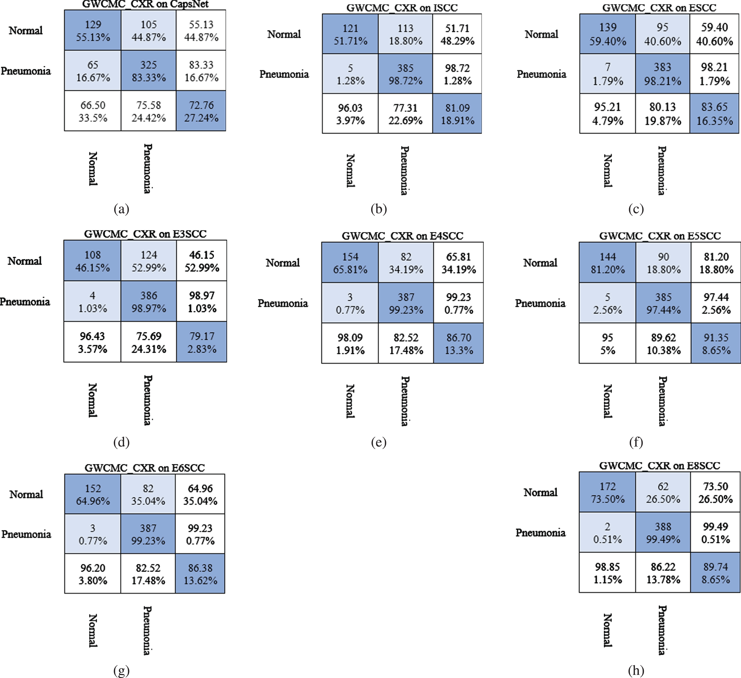
Confusion matrices for Pneumonia detection on GWCMC CXR images using (a) CapsNet, (b) Integrated skip convolutional capsule (ISCC), (c) Ensemble skip convolutional capsule (ESCC), (d) Ensemble of 3 skip convolutional capsule (E3SCC), (e) Ensemble of 4 skip convolutional capsule (E4SCC), (f) Ensemble of 5 skip convolutional capsule (E5SCC), (g) Ensemble of 6 skip convolutional capsule (E6SCC), and (h) Ensemble of 8 skip convolutional capsule (E8SCC).

5.3.2 RSNA

This section presents the accuracy using the RSNA data. The dataset was trained without any image modifications. The experiment conducted in this stage shows that the performance accuracy of our method is high compared to previous works.

In Table 4, we present the accuracy of the CapsNet, ISCC, ESCC and the variants models, based on the training, validation accuracy, train loss, validation loss, decoder train loss, decoder validation loss, total train loss and total validation loss. We observe that CapsNet converged at epoch 150 with the least score of 93.63%with high training parameters. In contrast, ISCC produced 95.95%with an improvement of 2.32%over the original CapsNet model. As alluded earlier, the integration of capsule network with skip convolution generates improve performance of the network. The ensemble networks (ESCC) and variants proves successful in the afore-mentioned intuition. We can see from Table 4 that the ensemble models constantly improve performance except for ESCC, which had least accuracy of 96.06%. The E6SCC and E8SCC achieved the remarkable accuracy of 98.98%and 999.85%, respectively. The models evaluation metrics (i.e. AUC and Pre_Rec, sensitivity, specificity) increasingly improves, which show how well the model generalized on the two classes (“Normal” and “Pneumonia”).

5.3.3 Mendeley chest X-ray

Table 5 presents the accuracy of the CapsNet, ISCC, ESCC and the variants models, based on the training, validation accuracy, train loss, validation loss, decoder train loss, decoder validation loss, total train loss and total validation loss. We observe that CapsNet converged at epoch 150 with the least score of 83.75%with high training parameters. In Fig. 15(a) of the confusion matrix, 9 instances were predicted as TNs (2.31%of the “Pneumonia” CXR images) and 381 instances (97.69%) predicted as TPs. In contrast, ISCC produced 90.71%with an improvement of 7.06%over the CapsNet model. This clearly explains that, integration of capsule network with skip convolution generates improve performance of the network. The ensemble networks (ESCC) and variants proves the afore-mentioned intuition. We can see from Table 5 that, the ensemble models constantly improve performance except for E3SCC, which had least accuracy of 88.30%. The E6SCC and E8SCC achieved the remarkable accuracy of 98.72%and 98.88%, respectively. The models metrics performance (i.e. AUC and Pre_Rec) increasingly improves, which show how well the model generalized on the two classes (“Normal” and “Pneumonia”). Figure 15 shows the confusion matrices for the models in Table 5, respectively. In Fig. 15(d) of the E3SCC model, the number of FNs predicted was 10 instances (2.56%of the “Pneumonia” CXR images) and 390 instances predicted as TPs (97.44%of the “Pneumonia” CXR images). However, 63 instances were predicted as FPs (26.9%of the “Normal” CXR images), which represent a person with no pneumonia infection hence predicted as pneumonia patients. In comparison to the best ensemble model (E8SCC), the E8SCC in Fig. 15(h) recorded 1 instance of TN (0.26%of the “Pneumonia” CXR images), which is pneumonia patients wrongly predicted as normal patients. This result is critical as a pneumonia patient may be denied of treatment and can result to death. Meanwhile, the model had 389 instances predicted as TPs (99.74%of the “Pneumonia” CXR images), which represent the true prediction of the patients with pneumonia. Furthermore, 6 instances were recorded as FPs (2.56%of the “Normal” CXR images), which is someone predicted to be pneumonia but do not actually have pneumonia. In summary, integration of skip convolutions, ensemble skip convolutions with capsules coupled with the proposed Algorithm 2, provided more importance information in the Mendeley CXR to achieve state-of-the-art performance. Detailed accuracies of the performance metric such as Precison_Recall, sensitivity, specificity, area under the curve (auc) and accuracy are shown in Table 5. It could be seen that the model was well generalized and achieve a good prediction on the test set.

Fig. 15

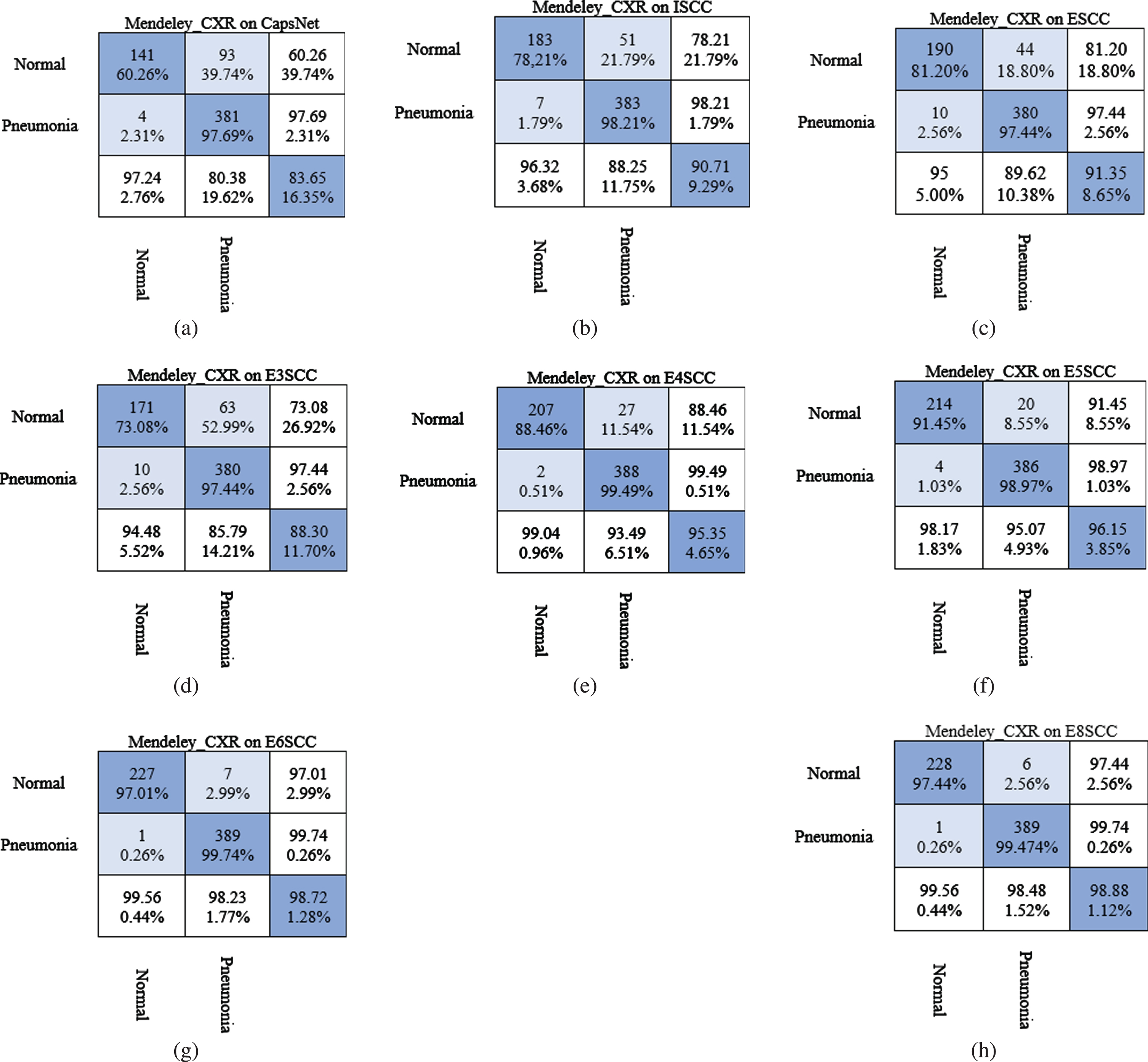
Confusion matrices for Pneumonia detection on Mendeley CXR dataset using (a) CapsNet, (b) Integrated skip convolutional capsule (ISCC), (c) Ensemble skip convolutional capsule (ESCC), (d) Ensemble of 3 skip convolutional capsule (E3SCC), (e) Ensemble of 4 skip convolutional capsule (E4SCC), (f) Ensemble of 5 skip convolutional capsule (E5SCC), (g) Ensemble of 6 skip convolutional capsule (E6SCC), and (h) Ensemble of 8 skip convolutional capsule (E8SCC).

5.4 Test prediction

In this section, we performed a test prediction to evaluate the efficiency of the model. In the prediction, capsule with the maximum length of vector is considered the output of the classifier. In order to evaluate the generalizability of the models, a comparison was done with the original image (ground truth). We used sample images from both classes (“Pneumonia” and “Normal”) as input to the predictive model for the prediction probabilities. Figure 16 shows result from the predictions. Figure 16 provides the probability per each class compared to the original image. We can observe that the dynamic routing coupled with the VSquash and our model performed well on the CXR images. Furthermore, the dynamic routing with VSquash produced high likelihood values for the per class prediction probabilities for each image. However, in our method produced 1 misclassification, where a “Normal” image was predicted as “Pneumonia” (see Fig. 16, column 2 row 4). This can be attributed to the similarity of image from the two classes. Overall, the prediction accuracies show that our method can effectively discriminate between the classes.

Fig. 16

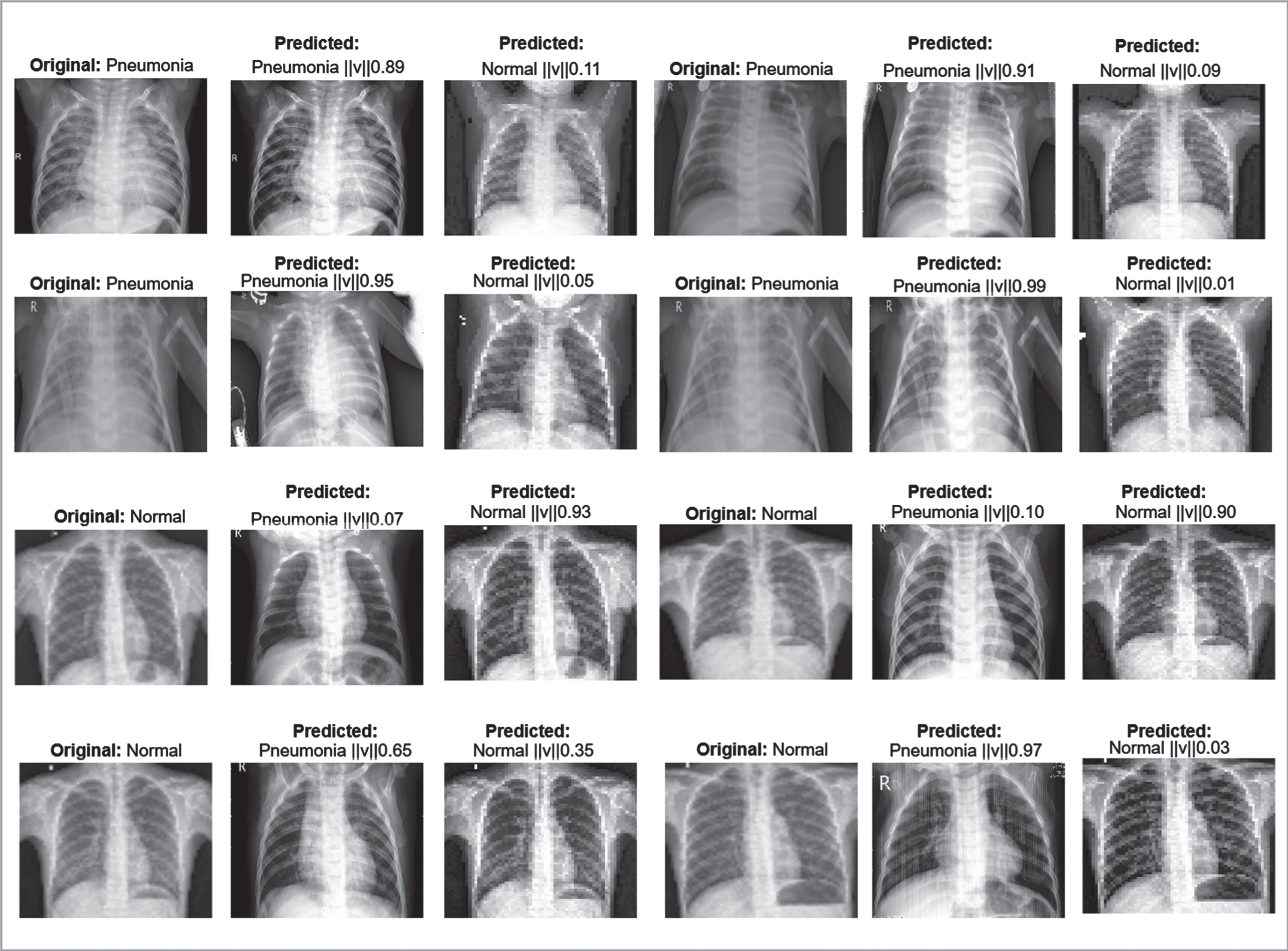
Visualizing prediction probability from our proposed method.

5.4.1 Confusion matrix

The confusion matrices that summaries the system’s performance for both studies conducted on the three datasets. The X-axis represents the predicted values (i.e. Model prediction) while the Y-axis indicates the true labels (ground truth/Actual). In the confusion matrices, the non-white columns show the actual classes and the non-white rows represent the output classes. Precision, Sensitivity, Specificity, and Accuracy have been calculated as in Equation (13)–(16).

Equation (13) shows the computation of precision, sensitivity, specificity and accuracy on our confusion matrix.

Precision = \frac{TP}{(TP + FP)}

(13)

Sensitivity = \frac{TP}{(TP + FN)}

(14)

Specificity = \frac{TN}{(TN + FN)}

(15)

Accuracy = \frac{TP + TN}{(TP + TN + FP + FN)}

(16)

Where, Precision: This metric indicates the proportion of positive identifications that was correct. We show the metric function Equation 14. High precision indicates an example labeled as positive case is positive.

Sensitivity (Recall): Unlike the precision, the recall shows proportion of actual positive samples that was correctly identified. Hence, it is used as measure to test the correctly generated positive result for actual pneumonia patients classified by the model. We mathematically define the recall in Equation 15. High recall shows that the class is correctly recognized (small number of FN). On the other hand, high recall with low precision shows most of the positive samples were correctly recognized (low FN) but there are more false positives. Whiles a low recall with high precision indicates miss of more positive examples (high FN) but the predicted positive sample are positive (low FP).

Specificity: measures the proportion of negative class that was correctly classified by the model. In contrast to Sensitivity, Specificity determines the proportion of healthy patients who were correctly identified by the model.

True Positive (TP) is the total number of predicted cases from the model indicating the patient have the pneumonia diseases.

True Negative (TN) is the total number of predicted cases from the model indicating the patient do not have the pneumonia diseases.

False Negative (FN) is the predicting outcome from the model showing the patient does not have the pneumonia disease; however, the patient does have the disease.

False Positive (FP) is the predicting outcome from the model showing the patient have the pneumonia disease; however, the patient does not have the disease.

6 Conclusion

In this work, a deep learning model named skip-connected convolutional capsules (S-CCCapsule) based on Capsule Networks architecture for pneumonia detection problem was presented. The skip-connection method transfers the input feature to each output of the high-level convolutional layers to keep more important information for better classification accuracy. Secondly, unlike squash function in [33], we proposed a new squash function called vertical squash (VSquash) to shrink vectors and prevent the activation values of the primary capsule in order to reduce non-informative capsules and promote the discriminative capsules. To obtain uniform distribution of routing coefficient of probabilities between capsules, we adopted Sigmoid function instead of Softmax function used in [33]. Ablation study was conducted on the S-CCCapsule model to see the effect of the CapsNet, which we arrived at three architectures (i.e. CapsNet+Maxpooling, BSCapsNet and LSCapsNet). Furthermore, integrated skip connected (ISCC), Ensemble architecture and its variants were implemented, which combine dense convolutions and capsules. For fair comparison, we implemented the original capsule network (CapsNet) and used as a baseline.

Our experiments were based on three public CXR datasets such as Guangzhou Women and Children’s Medical Center (GWCMC), Mendeley Chest X-Ray pneumonia and Radiological Society of North America (RSNA) images. The experimental result in the ablation study on the GWCMC, RSNA and Mendeley CXR images shows that S-CCCapsule achieves validation accuracy (CPNval) of 83.65%, 99.35%and 91.35%, respectively, compared to the other ablation models. Among the ISCC, ensemble models (ESCC), and its variants introduced in this work, the ISCC, ESCC and its four variants (E4SCC, E5SCC, E6SCC and E8SCC) produces best validation accuracy on the three datasets. We note that the introduction of skip connection, VSquash and Sigmoid enhanced the robustness of the models to overfitting and effectively generalized well on the images. Based on the experiment conducted, we can observe that the proposed method performed better compared to other methods. In addition, our designed architecture has shown to improve the accuracy in Pneumonia detection problem based on the presented confusion matrices.

Acknowledgment

This work was supported by National Natural Science Foundation of China (NSFC Grant No. 61550110248), Sichuan Science and Technology Program (Grant No.2019YFG0190) and Research on Sino-Tibetan multi-source information acquisition, fusion, data mining and its application (Grant No. H04W170186). The authors would like to thank the editor and the reviewers for their helpful suggestions and valuable comments.

Conflict of interest

The authors declare that they have no known competing financial interests or personal relationships that could have appeared to influence the work reported in this paper.

References

Boyle, https://www.cdc.gov/pneumonia/causes.html, 2018. [Online]. Available: https://www.cdc.gov/pneumonia/causes.html.

Franquet

, Imaging of pneumonia: Trends and algorithms, Eur Respir J 2001. doi: 10.1183/09031936.01.00213501.

Cherian

, et al., Standardized interpretation of paediatric chest radiographs for the diagnosis of pneumonia in epidemiological studies, Bull World Health Organ 2005. doi: /S0042-96862005000500011.

Anthimopoulos

, Christodoulidis

, Ebner

, Christe

and Mougiakakou

, Lung Pattern Classification for Interstitial Lung Diseases Using a Deep Convolutional Neural Network, IEEE Trans Med Imaging, 2016. doi: 10.1109/TMI.2016.2535865.

Jha

, Kumar

, Abdel-Basset

, Priyadarshini

, Sharma

and Long

H.V.

, Deep learning approach for software maintainability metrics prediction, IEEE Access 7 (2019), 61840–61855.

Pritam

, Khari

, Kumar

, Jha

, Priyadarshini

, Abdel-Basset

and Long

H.V.

, Assessment of code smell for predicting class change proneness using machine learning, IEEE Access 7 (2019), 37414–37425.

Jha

, Prashar

, Long

H.V.

and Taniar

, Recurrent neural network for detecting malware, Computers & Security 99 (2020), 102037.

Saxena

, Shukla

and Gyanchandani

, Pre-trained convolutional neural networks as feature extractors for diagnosis of breast cancer using histopathology, Int J Imaging Syst Technol, no. December 2019, 2020. doi: 10.1002/ima.22399.

, Adu

, Tashi

, Anokye

, Wang

and Ayidzoe

M.A.

, RMAF: ReLU-Memristor-like Activation Function for Deep Learning, IEEE Access 8 (2020), 72727–72741. doi: 10.1109/access.2020.2987829.

10.

Kumar

, Grewal

and Srivastava

M.M.

, Boosted Cascaded Convnets for Multilabel Classification of Thoracic Diseases in Chest Radiographs, in Lecture Notes in Computer Science (including subseries Lecture Notes in Artificial Intelligence and Lecture Notes in Bioinformatics), 2018. doi: 10.1007/978-3-319-93000-8_62.

11.

Rajpurkar

, et al., CheXNet: Radiologist-Level Pneumonia Detection on Chest X-Rays with Deep Learning, pp. 3–9, 2017.

12.

Wang

, Peng

, Lu

, Bagheri

and Summers

R.M.

, ChestX-ray8: Hospital-scale chest X-ray database and benchmarks on weakly-supervised classification and localization of common thorax diseases, in Proceedings - 30th IEEE Conference on Computer Vision and Pattern Recognition, CVPR 2017, 2017. doi: 10.1109/CVPR.2017.369.

13.

Albarqouni

, Baur

, Achilles

, Belagiannis

, Demirci

and Navab

, AggNet: Deep Learning From Crowds for Mitosis Detection in Breast Cancer Histology Images, IEEE Trans Med Imaging, 2016. doi: 10.1109/TMI.2016.2528120.

14.

, Mo

, Feng

, Zhong

, Lai

and Chang

E.I.C.

, Chang, Deep learning of feature representation with multiple instance learning for medical image analysis, in ICASSP, IEEE International Conference on Acoustics, Speech and Signal Processing – Proceedings, 2014. doi: 10.1109/ICASSP.2014.6853873.

15.

Liskowski

and Krawiec

, Segmenting Retinal Blood Vessels with Deep Neural Networks, IEEE Trans Med Imaging, 2016. doi: 10.1109/TMI.2016.2546227.

16.

Yuan

, Chao

and Lo

Y.C.

, Automatic Skin Lesion Segmentation Using Deep Fully Convolutional Networks with Jaccard Distance, IEEE Trans Med Imaging, 2017. doi: 10.1109/TMI.2017.2695227.

17.

Roth

H.R.

, et al., Deeporgan: Multi-level deep convolutional networks for automated pancreas segmentation, in Lecture Notes in Computer Science (including subseries Lecture Notes in Artificial Intelligence and Lecture Notes in Bioinformatics), 2015.

18.

, Cheng

, Xu

, Wong

D.W.K.

, Liu

and Cao

, Joint Optic Disc and Cup Segmentation Based on MultiLabel Deep Network and Polar Transformation, IEEE Trans Med Imaging, 2018. doi: 10.1109/TMI.2018.2791488.

19.

, et al., Segmentation and quantification for angle-closure glaucoma assessment in anterior segment oct, IEEE Trans Med Imaging, 2017. doi: 10.1109/TMI.2017.2703147.

20.

Yang

, Zhang

, Yan

, Tan

, Li

and Metaxas

, Automated anatomical landmark detection ondistal femur surface using convolutional neural network, in Proceedings –International Symposium on Biomedical Imaging, 2015. doi: 10.1109/ISBI.2015.7163806.

21.

Wolterink

J.M.

, Leiner

, Viergever

M.A.

and Išgum

, Generative adversarial networks for noise reduction in low-dose CT, IEEE Trans Med Imaging, 2017. doi: 10.1109/TMI.2017.2708987.

22.

Abdel-Basset

, Gamal

, Manogaran

and Long

H.V.

, A novel group decision making model based on neutrosophic sets for heart disease diagnosis, Multimedia Tools and Applications 28 (2019), 1–26.

23.

Sedai

, Mahapatra

, Ge

, Chakravorty

and Garnavi

, Deep multiscale convolutional feature learning for weakly supervised localization of chest pathologies in X-ray images, in Lecture Notes in Computer Science (including subseries Lecture Notes in Artificial Intelligence and Lecture Notes in Bioinformatics), 2018. doi: 10.1007/978-3-030-00919-9_31.

24.

Krizhevsky

, Sutskever

and Hinton

G.E.

, ImageNet classification with deep convolutional neural networks, in Advances in Neural Information Processing Systems, 2012.

25.

Krizhevsky

, Sutskever

and Hinton

G.E.

, ImageNet classification with deep convolutional neural networks, Commun ACM, 2017. doi: 10.1145/3065386.

26.

Simonyan

and Zisserman

, Very deep convolutional networks for large-scale image recognition, in 3rd International Conference on Learning Representations, ICLR 2015 –Conference Track Proceedings, 2015.

27.

Szegedy

, et al., Going deeper with convolutions, in Proceedings of the IEEE Computer Society Conference on Computer Vision and Pattern Recognition, 2015. doi: 10.1109/CVPR.2015.7298594.

28.

J.S.K.

, Zhang

and Ren

, Deep residual learning for image recognition, Proc IEEE Conf Comput Vis Pattern Recognit, no. Jun. 2016, pp. 770–778. doi: 10.3389/fpsyg.2013.00124.

29.

Yao

, Poblenz

, Dagunts

, Covington

, Bernard

and Lyman

, Learning to diagnose fromscratch by exploiting dependencies among labels, pp. 1–12, 2017.

30.

Huang

, Liu

, Van Der Maaten

and Weinberger

K.Q.

, Densely connected convolutional networks, in ,Proceedings –30th IEEE Conference on Computer Vision and Pattern Recognition, CVPR 2017, 2017. doi: 10.1109/CVPR.2017.243.

31.

Hochreiter

and Schmidhuber

, Long Short Term Memory, Neural Comput 1997. doi: 10.1162/neco.1997.9.8.1735.

32.

Jia

and Huang

, DE-CapsNet: A diverse enhanced capsule network with disperse dynamic routing, Appl Sci 2020. 10.3390/app10030884.

33.

Sabour

, Frosst

and Hinton

G.E.

, Dynamic routing between capsules, in Advances in Neural Information Processing Systems, 2017.

34.

, Zhang

, Ren

and Sun

, Deep residual learning for image recognition, in Proceedings of the IEEE Computer Society Conference on Computer Vision and Pattern Recognition, 2016. doi: 10.1109/CVPR.2016.90.

35.

Guan

, Huang

, Zhong

, Zheng

and Yang

Diagnose like a Radiologist: Attention Guided Convolutional Neural Network for Thorax Disease Classification

1 (2018), 1–10.

36.

Saul

C.J.

, Urey

D.Y.

and Taktakoglu

C.D.

, Early Diagnosis of Pneumonia with Deep Learning, 2019.

37.

Hashmi

M.F.

, Katiyar

, Keskar

A.G.

, Bokde

N.D.

and Geem

Z.W.

, Efficient pneumonia detection in chest xray images using deep transfer learning, Diagnostics, 2020. doi: 10.3390/diagnostics10060417.

38.

Mittal

, et al., Detecting pneumonia using convolutions and dynamic capsule routing for chest X-ray images, Sensors (Switzerland), 2020. doi: 10.3390/s20041068.

39.

Abiyev

R.H.

and Ma’aitah

M.K.S.

, Deep Convolutional Neural Networks for Chest Diseases Detection, J Healthc Eng, 2018. doi: 10.1155/2018/4168538.

40.

Stephen

, Sain

, Maduh

U.J.

and Jeong

D.U.

, An Efficient Deep Learning Approach to Pneumonia Classification in Healthcare, J Healthc Eng, 2019. doi: 10.1155/2019/4180949.

41.

Ayan

and Ünver

H.M.

, Diagnosis of pneumonia from chest X-ray images using deep learning, in 2019 Scientific Meeting on Electrical-Electronics and Biomedical Engineering and Computer Science, EBBT 2019, 2019. doi: 10.1109/EBBT.2019.8741582.

42.

Sabour

, Frosst

and Hinton

G.E.

, Dynamic Routing Between Capsules, no. Nips, 2017.

43.

Jiang

, Wang

, Liu

, Li

and Liu

, CapsNet, CNN, FCN: Comparative performance evaluation for image classification, Int J Mach Learn Comput, 2019. doi: 10.18178/ijmlc.2019.9.6.881.

44.

Patrick

M.K.

, Adekoya

A.F.

, Mighty

A.A.

and Edward

B.Y.

, Capsule Networks –A survey, Journal of King Saud University –Computer and Information Sciences, 2019. doi: 10.1016/j.jksuci.2019.09.014..

45.

Scherer

, Müller

and Behnke

, Evaluation of pooling operations in convolutional architectures for object recognition, in Lecture Notes in Computer Science (including subseries Lecture Notes in Artificial Intelligence and Lecture Notes in Bioinformatics), 2010. doi: 10.1007/978-3-642-15825-4_10.

46.

Akilan

, Wu

Q.J.

, Safaei

, Huo

and Yang

, A 3D CNN-LSTM-Based image-to-image foreground segmentation, IEEE Trans Intell Transp Syst, 2020. doi: 10.1109/TITS.2019.2900426.

47.

Huang

and Chen

, Li

, Wu

, van der Maaten

and Weinberger

K.Q.

, Multi-scale dense networks for resource efficient image classification, 2017. arXiv preprint arXiv:1703.09844.

48.

Iandola

F.N.

, Moskewicz

M.W.

, Ashraf

, Han

, Dally

W.J.

and Keutzer

, SqueezeNet, arXiv, 2016.

49.

Adu

, Yu

and Cai

, Dilated Capsule Network for Brain Tumor Type Classification ViaMRI Segmented Tumor Region, no. December, pp. 942–947, 2019.

50.

Shahroudnejad

, Afshar

, Plataniotis

K.N.

and Mohammadi

, Improved explainability of capsule networks: Relevance path by agreement, 2018 IEEE Glob. Conf. Signal Inf. Process. Glob. 2018 –Proc., pp. 549–553, 2019. doi: 10.1109/GlobalSIP.2018.8646474.

51.

Kermany

G.M.

, D, Labeled optical coherence tomography (OCT) and Chest X-Ray images for classification, Mendeley Data, 2018.

52.

Kingma

D.P.

and Ba

J.L.

, Adam: A method for stochastic optimization, in 3rd International Conference on Learning Representations, ICLR 2015 –Conference Track Proceedings, 2015.

53.

Sünderhauf

, Shirazi

, Dayoub

, Upcroft

and Milford

, On the performance of ConvNet features for place recognition, in IEEE International Conference on Intelligent Robots and Systems, 2015. doi: 10.1109/IROS.2015.7353986.

54.

Han

, Pool

, Tran

and Dally

W.J.

, Learning both weights and connections for efficient neural networks, in Advances in Neural Information Processing Systems, 2015.

55.

Xiang

, Zhang

, Tang

, Zou

and Xu

, MS-CapsNet: A Novel Multi-Scale Capsule Network, IEEE Signal Process Lett, 2018. doi: 10.1109/LSP.2018.2873892.

56.

Teh

Y.W.

and Hinton

G.E.

, Rate-coded restricted boltzmann machines for face recognition, in Advances in Neural Information Processing Systems, 2001.

57.

Zhang

and Sabuncu

M.R.

, Generalized cross entropy loss for training deep neural networks with noisy labels, arXiv preprint arXiv:1805.07836. 2018 May 20.