Machine learning prediction of concrete compressive strength with data enhancement

Abstract

The compressive strength of concrete can be predicted by machine learning. One thousand thirty samples of concrete compressive strength data were used as the dataset. Machine learning was applied to prediction of concrete compressive strength with seven machine learning algorithms. To improve data utilization and generalization ability of machine learning model, ten data sets were constructed by feature reorganization for data augmentation. Compared with other machine learning models, the XGBoost model based on Boosting tree algorithm had the highest prediction accuracy and the most robust generalization ability. With different multi-feature combination input conditions, the R² score of the XGBoost algorithm was 0.9283, the MAE score was 3.4292, the MAPE score was 12.5656, and the RMSE score was 5.2813. The error accumulation curve of the XGBoost algorithm was analyzed. When the compressive strength of concrete is at 5–20MPa, the error contribution rate is higher. When the concrete compressive strength is at 20–40MPa, the prediction result error of the model drops sharply. When the strength reaches 40MPa, the error contribution rate of the model tends to converge and the error contribution rate is stable between 1 and 1.2, which indicates that the model has high prediction accuracy when the compressive strength is higher than 40 MPa.

Keywords

Machine learning prediction of Compressive strength feature reorganization XGBoost data enhancement

1 Introduction

Due to high-performance concrete’s (HPC) excellent properties, HPC is widely used in various fields of construction industry [1, 2]. The 28-days compressive strength of concrete is reinforced concrete structure’s critical design parameter. Therefore, it is crucial to study compressive strength of concrete [3]. Due to the influence of components’ physicochemical properties, compressive strength of concrete varies significantly due to the different composition materials [4, 5]. The current compressive strength of concrete is obtained through test under given mix proportion scheme, which consumes many workforces, material, and financial resources. Simultaneously, industrial waste produced by waste concrete also brings a heavy burden to society. Therefore, it is valuable to study a reliable prediction model of concrete compressive strength [6].

With the rapid development of artificial intelligence technology, various industries combine with artificial intelligence technologies for self-empowerment [7 –11]. Based on computer vision technology, Ren Y P proposed a convolutional neural network for semantic segmentation of concrete cracks in tunnels, and achieved good results on the self-made tunnel crack data set, which provides a new idea for health monitoring tunnels and other structures [12]. J.K. Wilt established a deep learning model to predict the development of crack and explored the nonlinear relationship between crack stress and damage effect [13]. P.J. Chun proposed a supervised learning algorithm to evaluate internal damage of reinforced concrete structures [14]. R. Kulagin used machine learning algorithm to optimize chiral elements with large distortion and additional anisotropy requirements [15]. D. Daneshvar established dynamic elastic modulus prediction model of asphalt concrete using random forest algorithm, and the prediction accuracy can reach 94.62%[16]. S.S. Bangaru proposed an image segmentation method based on machine learning and applied it to the analysis of concrete SEM images. The results show that the image segmentation algorithm dramatically improves the accuracy and efficiency of SEM image analysis [17]. Engineering research based on machine learning is also in full swing [18]. Many machine learning algorithms have been applied to the study of concrete strength measurement, including artificial neural network [19], support vector machine [20, 21], and ensemble algorithm [6 , 23]. Based on four machine learning algorithms, V.Vakharia used cross-validation to predict concrete composition and used feature sorting to eliminate irrelevant features’ influence on the prediction results [6].

The research on the compressive strength of concrete based on machine learning is still in development stage, and there are some deficiencies in engineering application: 1. The existing research mostly only uses one of machine learning algorithms to predict the compressive strength of concrete [7 , 24–26]. However, few comparative studies on applicability of multiple algorithms on same data. 2. Most of the existing researches input multiple features into a model at one time, without considering the model’s generalization ability and robustness with different combination of features. 3. The utilization rate of existing literature for dataset is insufficient. Most literature didn’t reorganize features of dataset to achieve the data enhancement of text data. For the lack of previous researches, this paper constructed ten data sets through transformation and combination of eight input features. And the performance of seven machine learning models was compared and analyzed. The optimal prediction model of concrete compressive strength was built by comparing and analyzing the prediction results.

2 Dataset

The dataset used in this study are from the University of California’s machine learning laboratory, Irvine [27, 28]. This dataset consists of 1030 data points. Each data point contains eight characteristic inputs and one output, among which eight characteristic variables are: cement (kg/m³), age (days), water (kg/m³), coarse aggregate(kg/m³), fine aggregate (kg/m³), superplasticizer (kg/m³), fly ash (kg/m³), mineral powder (kg/m³). The output variable is the compressive strength of concrete. The statistics of numerical characteristics of the dataset are shown in Table 1. Q1, Q2, and Q3 represent the lower quartile, the middle quartile, and the upper quartile.

Table 1
Dataset feature statistics

Maximum Minimum Q1 Q2 Q3 Mean Standard Deviation

Cement 540.00 102.00 192.37 272.90 350.00 281.16 104.50

Blast Furnace Slag 359.40 0.00 0.00 22.00 142.95 73.89 86.28

Fly Ash 200.10 0.00 0.00 0.00 118.30 54.18 63.99

Water 247.00 121.80 164.90 185.00 192.00 181.56 21.35

Superplasticizer 32.20 0.00 0.00 6.40 10.20 6.20 5.97

CoarseAggregate 1145.00 801.00 932.00 968.00 1029.40 972.91 77.75

Fine Aggregate 992.60 594.00 730.95 779.50 824.00 773.58 80.17

Age 365.00 1.00 7.00 28.00 56.00 45.66 63.16

Compressive strength 82.60 2.33 23.71 34.44 46.13 35.81 16.70

	Maximum	Minimum	Q1	Q2	Q3	Mean	Standard Deviation
Cement	540.00	102.00	192.37	272.90	350.00	281.16	104.50
Blast Furnace Slag	359.40	0.00	0.00	22.00	142.95	73.89	86.28
Fly Ash	200.10	0.00	0.00	0.00	118.30	54.18	63.99
Water	247.00	121.80	164.90	185.00	192.00	181.56	21.35
Superplasticizer	32.20	0.00	0.00	6.40	10.20	6.20	5.97
CoarseAggregate	1145.00	801.00	932.00	968.00	1029.40	972.91	77.75
Fine Aggregate	992.60	594.00	730.95	779.50	824.00	773.58	80.17
Age	365.00	1.00	7.00	28.00	56.00	45.66	63.16
Compressive strength	82.60	2.33	23.71	34.44	46.13	35.81	16.70

3 Method of machine learning

3.1 Linear regression and polynomial regression

Linear regression describes output variables as a linear combination of characteristic matrices. This linear combination is a hyperplane in n-dimensional space. The numerical solution of linear regression is the hyperplane that minimizes the square error between true value and predicted value [29]. The mathematical definition of linear regression is as follows: $\hat{y} = x^{T} β + ɛ$ (1)

Where: x is the characteristic matrix of the input, β is the coefficient matrix of linear model, ɛ is the error term of linear model, $\hat{y}$ is the output vector of the linear model.

Polynomial regression uses the n-degree polynomial of input variables to predict the output. Taking quadratic polynomial regression as an example, the mathematical expression of polynomial regression is as follows: $\hat{y} = β_{11} x_{1}^{2} + β_{22} x_{2}^{2} + β_{12} x_{1} x_{2} + β_{1} x_{1} + β_{2} x_{2} + β_{0}$ (2)

3.2 Support vector regression (SVR)

For sample (x, y), model constructed by linear and polynomial regression makes the model’s predicted value as close as possible to true value. When predicted value is equal to the true value, the result of loss function is zero. However, support vector regression (SVR) algorithm is different. SVR is based on two principles [30]: 1. The model can allow the error (ɛ) between predicted value and true value; 2. when the absolute error between predicted value and true value is greater than ɛ, the model’s loss function will be updated. Therefore, SVR model takes f (x) as the center and ±ɛ as bandwidth. The schematic diagram of SVR is shown in Fig. 1. The mathematical function of SVR is as follows [9]:

Fig. 1

Principle diagram of SVR.

$min_{ω, b} \frac{1}{2} ∥ ω ∥^{2} + C \sum_{i = 1}^{m} L (f (x_{i}) - y_{i})$ (3)

where: ω is the normal vector, C is the regularization constant, L is the damage function of the model, f (x_i) is the predicted value of the model, y_i is true value.

3.3 Regression decision tree

Regression decision tree (DT) refers to CART (classification and regression tree) composed of root node, child node, and leaf node [31]. The values of decision tree’s internal node characteristics are only “yes” and “no”. Therefore, decision tree is also a binary tree structure. The decision regression tree determines output value according to the eigenvector. The feature space is divided into different regions by two classification conditions to realize each region’s prediction and regression. In decision tree model, each node’s splitting criterion is determined by generated node’s purity. The node splitting is conducted along the direction to maximize the purity gain. The G (D, a) (information gain) is usually selected as the index to measure the process. The mathematical definition of G (D, a) is shown in equations (5). The regression principle of decision tree is shown in Fig. 2.

Fig. 2

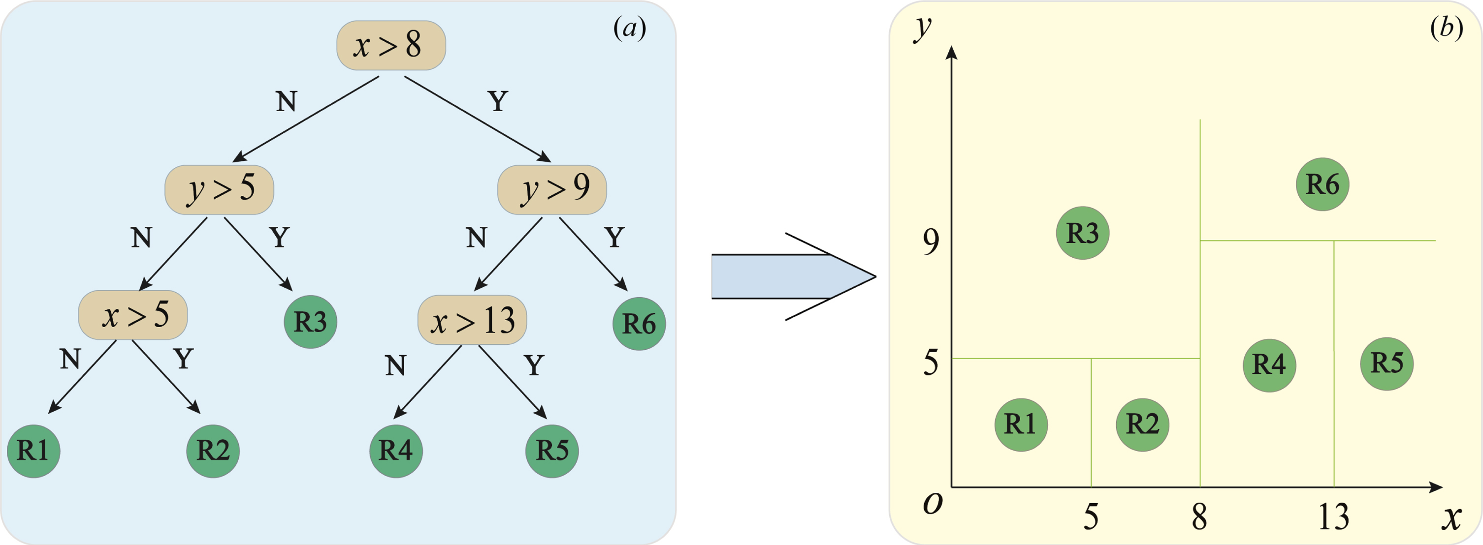
Schematic diagram of decision tree.

$H (D) = - \sum_{k = 1}^{| y |} p_{k} {log}_{2}^{P_{k}}$ (4) $G (D, a) = H (D) - \sum_{v = 1}^{V} \frac{| D^{v} |}{| D |} H (D^{v})$ (5) where: P_k is represents the proportion of class k, H (D) is represents the information entropy of set D, a is the attribute category selected for information gain.

3.4 Bagging algorithm

Bagging algorithm is the representative of parallel ensemble algorithm. For a given original data set with n samples, a train set composed of M samples is obtained by Bootstrap Sample. The same sampling process is carried out for K times to get K train sets. Then a primary learner is trained based on each train set. Bagging algorithm obtains each base learner’s prediction results by train k independent base learners. Finally prediction results of the whole ensemble algorithm will be calculated by voting the prediction results of K base learners [32].

In this study, the bagging ensemble algorithm is Random forest(RF) using for regression analysis of data sets. RF is a modified bagging ensemble algorithm which consists of integrating several decision trees. At the same time, the random selection of feature attributes is introduced in the train process of decision tree for RF [33]). Based on this mechanism, RF inherits the sample disturbance advantage of bagging ensemble algorithm and introduces the disturbance strategy of attribute random selection to improve model generalization ability. The algorithm principle of random forest is shown in Fig. 3.

Fig. 3

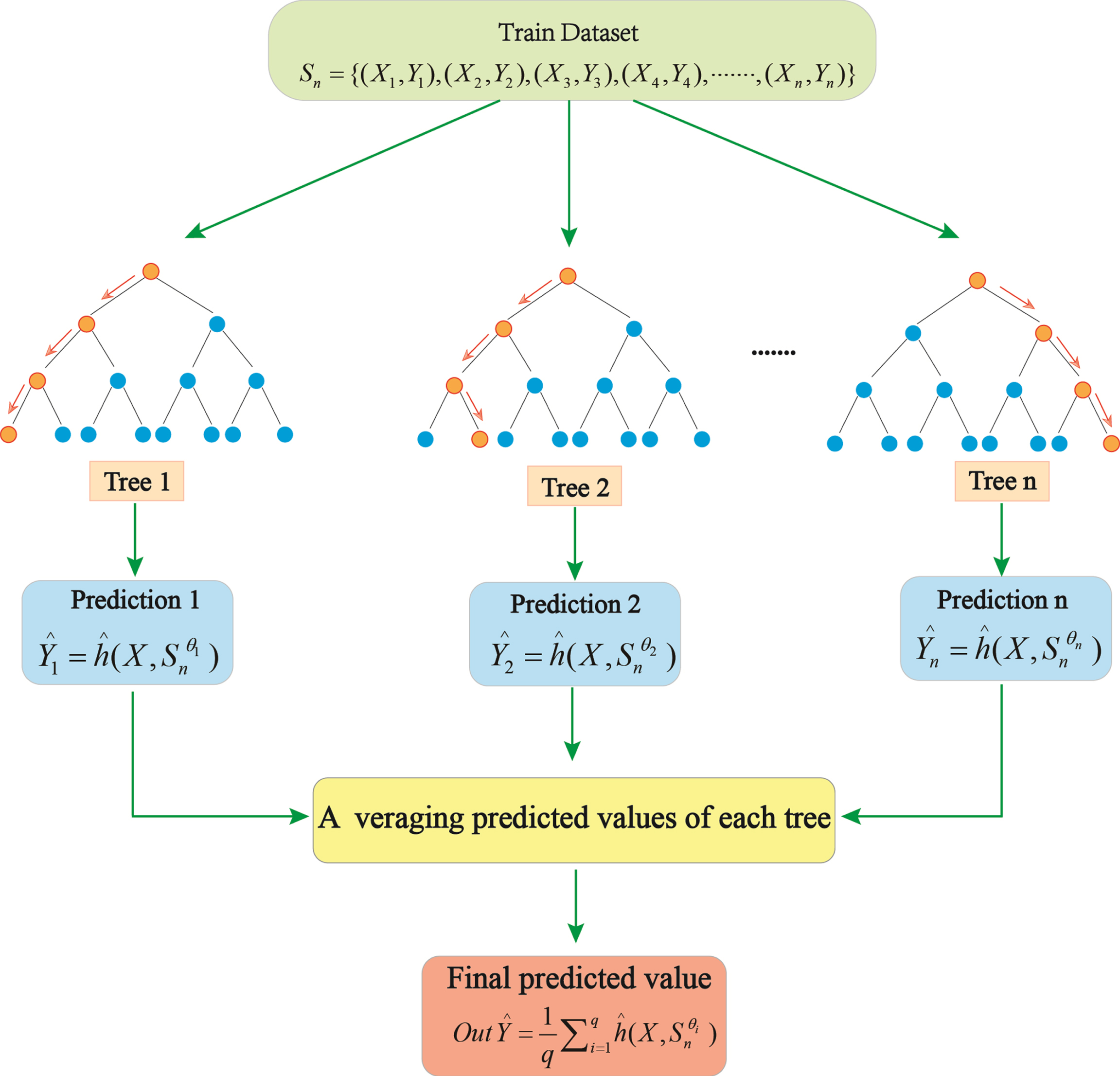
Principle of random forest algorithm.

3.5 Boosting algorithm

Different from the parallel ensemble algorithm of RF, boosting algorithm is an algorithm that improves weak learner to strong learner. Mechanism of boosting algorithm is as follows: firstly, a weak learner is used to build the model, and the weak learner is trained on train set. Secondly, parameters are adjusted according to the first learner’s performance on train set. Then next model is learned according to residual error of the first model. The samples with the former base learner’s inaccurate prediction will get more attention in latter base learner and the latter will be trained. The performance of the model is always improved and the model’s learning ability is enhanced [34]. Finally the iterative operation based on the residuals of the previous model will be repeated until meeting preset requirements. The boosting algorithms used in this paper are XGBoost and GradientBoost(GBR).

4 Model evaluation

4.1 Evaluating indicator

To compare and measure each machine learning algorithm’s performance on the same dataset, this paper selects four typical model evaluation indicators (R2, MAE, MAPE, RMSE). The mathematical definition of each indicators are shown in Table 2.

Table 2
Model evaluation indexes

Measures Parameter Description

MAE $MAE = \frac{1}{n} \sum_{i = 1}^{n} | y^{'} - y |, \in [0, + \infty)$ MAE uses the mean value of the absolute value of the error to measure the model’s prediction accuracy. The unit of MAE is MPa, which can directly reflect the physical meaning of the error to a certain extent. MAE measures the median error of the model, the smaller the value, the higher the model’s prediction accuracy. Where is the predicted value is y′ and the true value is y.

R2 $R^{2} = \frac{\sum_{i} ({\hat{y}}_{i} - \bar{y})}{\sum_{i} (y_{i} - \bar{y})}, \in [0, 1]$ In this paper, the default value of cross-validation results is used. The larger the R², the greater the error fluctuation of the model prediction results.

MAPE $MAPE = \frac{1}{n} \sum | \frac{y - y^{'}}{y} |, \in [0, + \infty)$ MAPE divides the true value of the label based on MAE, and measures the proportion of error in the whole true value in the form of proportion.

RMSE $RMSE = \sqrt{\frac{1}{n} \sum_{i = 1}^{n} {(y^{'} - y)}^{2}, \in [0, + \infty)}$ The dimension of RMSE is the same as MAE. From the definition of the two, MAE measures the true error of the model, while RMSE calculates the square based on the error, which is equivalent to increasing the weight of the influence of large number on the final results. Therefore, RMSE is more sensitive to outliers and is a supplement to measure MAE.

Measures	Parameter	Description
MAE	$MAE = \frac{1}{n} \sum_{i = 1}^{n} \| y^{'} - y \|, \in [0, + \infty)$	MAE uses the mean value of the absolute value of the error to measure the model’s prediction accuracy. The unit of MAE is MPa, which can directly reflect the physical meaning of the error to a certain extent. MAE measures the median error of the model, the smaller the value, the higher the model’s prediction accuracy. Where is the predicted value is y′ and the true value is y.
R2	$R^{2} = \frac{\sum_{i} ({\hat{y}}_{i} - \bar{y})}{\sum_{i} (y_{i} - \bar{y})}, \in [0, 1]$	In this paper, the default value of cross-validation results is used. The larger the R², the greater the error fluctuation of the model prediction results.
MAPE	$MAPE = \frac{1}{n} \sum \| \frac{y - y^{'}}{y} \|, \in [0, + \infty)$	MAPE divides the true value of the label based on MAE, and measures the proportion of error in the whole true value in the form of proportion.
RMSE	$RMSE = \sqrt{\frac{1}{n} \sum_{i = 1}^{n} {(y^{'} - y)}^{2}, \in [0, + \infty)}$	The dimension of RMSE is the same as MAE. From the definition of the two, MAE measures the true error of the model, while RMSE calculates the square based on the error, which is equivalent to increasing the weight of the influence of large number on the final results. Therefore, RMSE is more sensitive to outliers and is a supplement to measure MAE.

4.2 Feature importance analysis

The importance of variables in the dataset are shown in Fig. 4. According to the order of importance, eight input features are artificially divided into three levels: important feature, medium feature and weak feature. Cement dosage and Age are important features. The features of Water and Blast Furnace Slag are medium features, and remaining four input variables are weak features. To eliminate the randomness of model performance caused by a single dataset, the eight input variables are recombined according to the rule shown in Table 3. It is found that there must be at least one important feature in each feature combination. Otherwise, considerable error caused by one feature combination will cover up other combinations. The comparison of the seven machine learning algorithms used in this paper is based on average performance results of Table 3.

Fig. 4

Statistics of importance of features.

Table 3

Combination of characteristic variables of the data set

	C	Age	W	BFS	CA	FA	SP	Ash
FC1	√	√	√	√	√	√	√	√
FC2	√	√	√	√			√	√
FC3	√	√	√	√	√	√
FC4	√	√	√	√
FC5	√	√					√	√
FC6	√	√			√	√
FC7	√		√	√			√	√
FC8	√		√	√	√	√
FC9		√	√	√			√	√
FC10		√	√	√	√	√

4.3 Cross-validation

Machine learning model is generally trained on train set and gets the model’s updated weight parameters. To measure the trained model’s prediction accuracy for other datasets, it needs to be tested and evaluated on test set. The performance of the model on the test set determines generalization ability of the model. To set up train and test set, the typical way is to divide the original data set into train set and test set according to a certain proportion. These two parts are mutually exclusive and complementary. However, due to Bootstrap Sample’s randomness, many samples have not participated in the model train from the beginning to the end, which is a massive waste for the dataset [35]. Therefore, this paper uses k-fold cross-validation to overcome that shortcoming. The schematic diagram of k-fold cross-validation is shown in Fig. 5.

Fig. 5

Schematic diagram of K-fold cross-validation.

Figure 5 shows that each part of original dataset participates in train or test of the model in the whole process. Therefore, k-fold cross-validation gives full play to each dataset’s value without causing data waste. The segmentation parameter of k-fold cross-validation in this paper is 10. The dataset is divided into ten samples each time, nine samples are used as train set, and other one is used as test set [36].

5 Results and analysis

5.1 Comparison of model results

In order to make each model optimal, this paper uses the Grid-search to optimize the parameters of each models. Simultaneously, to compare the model’s generalization ability on different combinations of characteristic variables, seven algorithms’ performance adopt average value on the feature combination system in Table 3. Based on the model evaluation system established above, each model’s final results are statistically analyzed and the comparison results are shown in Fig. 6.

Fig. 6

Comparison and analysis of model results: (a)MAE, (b)MAPE, (c)RMSE, (d)R².

XGBoost and GBR based on boosting algorithm perform best in the dataset from the four rating indicators’ overall score. Random forest is third; the SVR and decision tree model performance is almost equal. The remaining linear regression and polynomial regression prediction errors are massive. The linear regression model’s performance is the worst, and the polynomial expression ability is slightly better than linear. In a sense, this shows that the multivariable input and output of the dataset are highly nonlinear. From the model’s error fluctuation, the standard deviation of the XGBoost model is the smallest, which indicates that the XGBoost model has better robustness and better generalization ability with different combination conditions.

5.2 Analysis of prediction results of XGBoost model

The R2 of the XGBoost on the FC1 feature combination test set is 0.9263, MAE is 2.64MPa, MAPE is 10.01%, RMSE is 4.63 MPa. The statistical results of XGBoost prediction and true value are shown in Fig. 7. The following conclusion can be drawn from Fig. 7(a). For different compressive strength of concrete, the prediction results of the XGBoost model are very close to true values of test set, and the errors of all prediction results are controlled within 12%, and most of the errors are within 6%. The following conclusion can be drawn from Fig. 7(b). Most of the data predictions of XGBoost are within±10%. According to statistics, there are 309 samples on the FC1 feature combination test set, among which 204 samples have prediction results within±10%, and 105 samples which is called error overrun point have error more than±10%. Error overrun points are mostly distributed in areas with low concrete compressive strength. The error of samples with higher strength is smaller. The model may be more accurate for data points with higher strength.

Fig. 7

Analysis of XGBoost prediction results: (a) Error scatter plot, (b) Analysis of±10%error.

5.3 Error contribution analysis of XGBoost model

In order to verify the conclusion that the XGBoost model mentioned can accurately predict the data with higher strength and the prediction error of data with lower strength is more massive. In this section, the error of the XGBoost model is analyzed in depth. To evaluate the error distribution of data more scientifically and reasonably, it is necessary to define error measurement indicators. This paper’s data are particular because of the uneven distribution of the data points in this paper. More samples in the lower strength range and fewer samples in higher strength range lead to two potential error mode: 1, “ many a little make a mickle”. That is to say, there are many samples in the low-strength region, and the error will have a cumulative effect on the model error after each sample being accumulated. 2. The error weight of low-strength samples is high; that is, the inaccurate prediction of low-strength samples mainly causes the model error. This paper introduces the error contribution rate(EC) to determine which error mode affects the error of the XGBoost model. The definition of EC is shown in formula (6). Taking the set of FC1 test set with concrete compressive strength less than 30MPa as an example.Taking the error of±10%as the error limit point, the total number of samples in this set is 120, the number of out of limit samples is 58, and the total number of samples of train set is 309. This set contributes 55.24%of the whole model’s error with 38.83%of the sample occupancy rate, which shows that the prediction error of the XGBoost model is large when the strength is less than 30MPa. $E_{c} = \frac{N_{o} / M_{o}}{N_{s} / M_{s}}$ (6)

Where: N_o is the number of overrun points in a set, N_s is the number of samples in the set, M_o is total number of overrun points in the model, M_s is total sample number of the model.

The statistical error results of the XGBoost model on the FC1 test set are shown in Fig. 8. What can be seen from Fig. 8 is following. When the model error accumulates are close to 50%, the corresponding concrete compressive strength is 27.42 MPa. With increase of compressive strength, the error accumulation curve’s tangent slope gradually decreases. Overall, the conclusion that the XGBoost model has more massive prediction error for low strength samples is correct. It can be seen from the error contribution rate curve in Fig. 8 that error contribution rate is higher when the compressive strength of concrete is 5–20MPa. When the concrete compressive strength is at 20–40MPa, the prediction result error of the model drops sharply. When the strength reaches 40MPa, the error contribution rate of the model tends to converge and the error contribution rate is stable between 1 and 1.2, which indicates that the model has high prediction accuracy when the compressive strength is higher than 40 MPa.

Fig. 8

Error curve of the XGBoost Model.

6 Conclusion

Prediction of HPC’s Strength is a challenging task. In this paper, seven machine learning algorithms were used to predict compressive strength of concrete. The purpose of this paper is to develop a reliable prediction model. Several conclusions can be drawn:

By reorganizing the characteristic variables of the dataset, ten datasets are established to realize data enhancement. It provides a new idea for data enhancement of structured data similar to this study.

It is found that the XGBoost algorithm has the highest prediction accuracy and generalization ability. The average R2 of XGBoost is 0.9283. The XGBoost algorithm can be applied to the compressive strength prediction of HPC.

XGBoost algorithm has high prediction accuracy for concrete strength above 40MPa and relatively large prediction error for concrete samples below 40MPa.

Footnotes

Acknowledgments

This work was supported by the National Nature Science Foundation of China (Grant Nos. 51768033, 51808272); Gansu Province guide science and technology innovation and development special project - key research and development ability improvement project(2019ZX-09) , and “Innovation star” project of excellent postgraduates in Gansu Province(2021CXZX-572).

Conflict of interest

The authors declare no conflict of interest.

ORCID: Xiaoning CUI

References

Chiew

F.H.

, Ng

C.K.

, Chai

K.C.

and Tay

K.M.

, A Fuzzy Adaptive Resonance Theory-Based Model for Mix Proportion Estimation of High-Performance Concrete, Computer Aided Civil & Infrastructure Engineering 32(9) (2017), 772–786.

Wetzel

and Middendorf

, Influence of silica fume on properties of fresh and hardened ultra-high performance concrete based on alkali-activated slag, Cement and Concrete Composites 100 (2019), 53–59.

Lim

C.H.

, Yoon

Y.S.

and Kim

J.H.

, Genetic algorithm in mix proportioning of high-performance concrete, Cement & Concrete Research 34(3) (2004), 409–420.

Chang

T.P.

, Chuang

F.C.

and Lin

H.C.

, A mix proportioning methodology for high-performance concrete, Journal of the Chinese Institute of Engineers 19(6) (1996), 645–655.

Bharatkumar

B.H.

, Narayanan

, Raghuprasad

B.K.

and Ramachandramurthy

D.S.

, Mix proportioning of high performance concrete, Cement & Concrete Composites 23(1) (2001), 71–80.

Vakharia

and Gujar

, Prediction of compressive strength and portland cement composition using cross-validation and feature ranking techniques, Construction and Building Materials 225 (2019), 292–301.

Choi

, Shin

, Jung

, Bae

H.J.

and Kim

, Convolutional Neural Network Technology in Endoscopic Imaging: Artificial Intelligence for Endoscopy, Clinical Endoscopy 53(2) (2020), 117–126.

Asadi

, Gindy

and Alvarez

, A Machine Learning Based Approach for Automatic Rebar Detection and Quantification of Deterioration in Concrete Bridge Deck Ground Penetrating Radar B-scan Images, KSCE Journal of Civil Engineering 23(6) (2019), 2618–2627.

Aiyer

B.G.

, Kim

, Karingattikkal

, Samui

and Rao

P.R.

, Prediction of compressive strength of self-compacting concrete using least square support vector machine and relevance vector machine, Ksce Journal of Civil Engineering 18(6) (2014), 1753–1758.

10.

Liu

J.C.

and Zhang

, Prediction of Explosive Spalling of Heated Steel Fiber Reinforced Concrete using Artificial Neural Networks, Journal of Advanced Concrete Technology 18(5) (2020), 227–240.

11.

Kim

D.-H.

, Kim

T.J.Y.

, Wang

, Kim

, Quan

Y.-J.

, Oh

J.W.

, Min

S.-H.

, Kim

, Bhandari

, Yang

and Ahn

S.-H.

, Smart Machining Process Using Machine Learning: A Review and Perspective on Machining Industry, International Journal of Precision Engineering and Manufacturing-Green Technology 5(4) (2018), 555–568.

12.

Ren

, Huang

, Hong

, Lu

and Shen

, Image-based concrete crack detection in tunnels using deep fully convolutional networks, Construction and Building Materials 234 (2020), 117367.

13.

Wilt

J.K.

, Yang

and Gu

G.X.J.A.E.M.

, Accelerating Auxetic Metamaterial Design with Deep Learning, (2020), 1901266.

14.

Chun

P.J.

, Ujike

, Mishima

, Kusumoto

and Okazaki

, Random forest-based evaluation technique for internal damage in reinforced concrete featuring multiple nondestructive testing results, Construction and Building Materials 253 (2020), 119238.

15.

Kulagin

, Beygelzimer

, Estrin

, Schumilin

and Gumbsch

P.J.A.E.M.

, Architectured Lattice Materials with Tunable Anisotropy: Design and Analysis of the Material Property Space with the Aid of Machine Learning, Advanced Engineering Materials (2020), 2001069.

16.

Daneshvar

and Behnood

, Estimation of the dynamic modulus of asphalt concretes using random forests algorithm, International Journal of Pavement Engineering (2020), 1–11.

17.

Bangaru

S.S.

, Wang

, Hassan

, Jeon

H.W.

and Ayiluri

, Estimation of the degree of hydration of concrete through automated machine learning based microstructure analysis –A study on effect of image magnification, Advanced Engineering Informatics 42 (2019), 100975.

18.

Pan

, Gui

, Lin

and Yan

, Deep BBN Learning for Health Assessment toward Decision-Making on Structures under Uncertainties, KSCE Journal of Civil Engineering 22(3) (2018), 928–940.

19.

Chithra

, Kumar

S.R.R.S.

, Chinnaraju

and Alfin

, Ashmita, A comparative study on the compressive strength prediction models for High Performance Concrete containing nano silica and copper slag using regression analysis and Artificial Neural Networks, Construction and Building Materials 114 (2016), 528–535.

20.

Chou

J.S.

and Pham

A.D.

, Smart Artificial Firefly Colony Algorithm-Based Support Vector Regression for Enhanced Forecasting in Civil Engineering, Computer-Aided Civil and Infrastructure Engineering 30(9) (2015), 715–732.

21.

Khazaeeu

and Ghalehnovi

, Bearing Stiffness of UHPC; An Experimental Investigation and A Comparative Study of Regression and SVR-ABC Models, Journal of Advanced Concrete Technology 16(3) (2018), 145–158.

22.

Han

, Gui

, Xu

and Lacidogna

, A generalized method to predict the compressive strength of high-performance concrete by improved random forest algorithm, Construction and Building Materials 226 (2019), 734–742.

23.

DeRousseau

M.A.

, Laftchiev

, Kasprzyk

J.R.

, Rajagopalan

and Srubar

W.V.

, A comparison of machine learning methods for predicting the compressive strength of field-placed concrete, Construction and Building Materials 228 (2019), 116661.

24.

Gilan

S.S.

, Jovein

H.B.

and Ramezanianpour

A.A.

, Hybrid support vector regression –Particle swarm optimization for prediction of compressive strength and RCPT of concretes containing metakaolin, Construction & Building Materials 34 (2012), 321–329.

25.

Marta

, Iñaki

F.O.

and Angel

, Neural network prediction of unconfined compressive strength of coal fly ash–cement mixtures, Cement and Concrete Research 33(8) (2003), 1137–1146.

26.

Chou

J.S.

and Pham

A.D.

, Enhanced artificial intelligence for ensemble approach to predicting high performance concrete compressive strength, Construction & Building Materials 49 (2013), 554–563.

27.

Yeh

I.C.

, Modeling of strength of high-performance concrete using artificial neural networks, Cement and Concrete Research 28(12) (1998), 1797–1808.

28.

Yeh

I.C.

, Optimization of concrete mix proportioning using a flattened simplex–centroid mixture design and neural networks, Engineering with Computers 25(2) (2009), 179–190.

29.

Seber, Linear regression analysis, Technometrics 45(4) (2003), 362–363.

30.

Drucker

, Burges

, Kaufman

, Smola

and Vapnik

, Support vector regression machines, Advances in Neural Information Processing Systems 9(7) (2003), 779–784.

31.

Loh

W.Y.

, Classification and regression trees, Wiley Interdiplinary Reviews: Data Mining and Knowledge Discovery 1 (2011), 14–23.

32.

Breiman

, Bagging Predictors, Machine Learning 24(2) (1996), 123–140.

33.

Breiman

, Random Forests, Machine Learning 45(1) (2001), 5–32.

34.

Ayyadevara

V.K.

, Gradient Boosting Machine, Pro Machine Learning Algorithms : A Hands-On Approach to Implementing Algorithms in Python and R, Apress, Berkeley, CA, 2018, 117–134.

35.

Vakharia

, Gupta

V.K.

and Kankar

P.K.

, Efficient fault diagnosis of ball bearing using ReliefF and Random Forest classifier, Journal of the Brazilian Society of Mechanical Sciences and Engineering 39(8) (2017), 2969–2982.

36.

Chou

J.-S.

, Tsai

C.-F.

, Pham

A.-D.

and Lu

Y.-H.

, Machine learning in concrete strength simulations: Multi-nation data analytics, Construction and Building Materials 73 (2014), 771–780.