Autonomous obstacle avoidance of UAV based on deep reinforcement learning 1

Abstract

In the intelligent unmanned systems, unmanned aerial vehicle (UAV) obstacle avoidance technology is the core and primary condition. Traditional algorithms are not suitable for obstacle avoidance in complex and changeable environments based on the limited sensors on UAVs. In this article, we use an end-to-end deep reinforcement learning (DRL) algorithm to achieve the UAV autonomously avoid obstacles. For the problem of slow convergence in DRL, a Multi-Branch (MB) network structure is proposed to ensure that the algorithm can get good performance in the early stage; for non-optimal decision-making problems caused by overestimation, the Revise Q-value (RQ) algorithm is proposed to ensure that the agent can choose the optimal strategy for obstacle avoidance. According to the flying characteristics of the rotor UAV, we build a V-Rep 3D physical simulation environment to test the obstacle avoidance performance. And experiments show that the improved algorithm can accelerate the convergence speed of agent and the average return of the round is increased by 25%.

Keywords

UAV obstacle avoidance DQN overestimation convergence rate

1 Introduction

UAV has been widely used in military and civilian fields because of its high cost performance, good flexibility, and freedom from pilot physiological conditions. With the operating airspace of drones continues to expand from medium and high altitudes to low altitudes, the complexity of the obstacle environment faced by drones has gradually increased [1]. Since the low-altitude obstacle environment is dense, dynamic and uncertainty [2], the complex obstacle environment brings great challenges to the flight safety of drones [3, 4].

At present, there are five types of UAV obstacle avoidance methods: methods based on mathematical planning, methods based on Voronoi diagram, methods based on spatial decomposition, methods based on potential fields, and methods based on machine learning.

Mathematical planning refers to the process of finding the optimal solution of the objective function under a series of constraints [5]. However, it is difficult to calculate when the dynamic or environmental constraints are complex [6]. The basic idea of Voronoi diagram [7] method is to draw polygons around obstacles to form Voronoi diagram and ensure the maximum distance between path and threat. The principle of Voronoi diagram is essentially a two-dimensional route planning algorithm and the planned route does not meet the kinematic constraints of aircraft [8]. The space decomposition method decomposes the task space into regular-shaped units, and judges whether the units are covered by obstacles or intersect with obstacles. In recent years, it has been more and more used in UAV route planning, such as Genetic Algorithm (GA) [9], particle swarm optimization (PSO) [10], whale optimization algorithm (WOA) [11], ant lion optimizer (ALO) [12], pigeon Inspi Optimization (PIO) [13]. However, these methods need a lot of computing resources and is difficult to guarantee the real-time of path planning in complex scenarios. The method based on the potential field performs planning by modeling the planning space as an area with different potential fields, and then a path search is performed in the potential field area [14]. In order to solve the problem of UAV’s flight path planning, references [15] and [16] combine UAV kinematics model with artificial potential field method, so as to make the planning route more in line with the kinematic characteristics of UAV. But the method based on the potential field is easy to fall into local minimum.

In recent years, the concept of the Reinforcement Learning (RL) [17] was proposed. With the development of time, Q-Learning [18], SARSA [19], Deep Q-learning Network (DQN) [20] and other RL algorithms have been proposed, but the table data recording method has obvious limitations in action and state space. Several improvements based on DQN have proposed in recent years [21 –25], including Dueling network structure [21], Double network structure [22] and complex empirical sampling policy [23]. Wang. Z et al. [21] introduced the dueling mechanism and proposed the Dueling Deep Q network (Dueling-DQN). Some scholars [22] have proposed Deep Double Q-Network (DDQN), which uses two sets of different network parameters to select actions and to evaluate the optimal Q-value separately. Schaul et al. [23] proposed an experience playback mechanism based on DQN to improve the sample utilization rate. Narasimhan et al. [26] combined LSTM and DQN, and proposed LSTM-DQN with time-dimensional memory. Subsequently, experiments [27] have been done on Atari 2600 to verify the generality of this method in visual perception. Lample [28] and Schulze [29] have used RL agent to play ViZDoom game and verified the good navigation decision ability of DQN.

Most scholars only verify the algorithm in the game environment, but few scholars combine reinforcement learning with practical application. Chen et al. [30] used RL algorithm for ship control. Wu et al. [31] used DQN to control robot motion automatically. Besides, Xie [32] improved the experience replay mechanism for UAV path planning, and speed up the convergence of reinforcement learning models. Wang et al. [33] used the sparse reward ensures that the RL solution is not biased toward potentially suboptimal directions. Omar et al. [34] study the RL’s trajectories of UAV in different scenarios.

However, the above algorithms mostly use a single sensor and ignore role of other sensors. At the same time, the above algorithm does not further optimize the convergence speed of the algorithm and the optimality of the agent strategy. This article uses image and distance data as input and propose the optimization method of the model from network structure and training policy. It is hoped that the agent can find the shortest path to the target position without collision. The contributions of this article are as follows:

The end-to-end sensor fusion. In this paper, distance information and visual information are adaptively fused to realize end-to-end obstacle avoidance of multiple sensors.

Improve the network structure. Use multiple parallel dueling neural network branches to select the optimal strategy by voting and scoring. The Q value is calculated through multiple weakly correlated network branches, and each branch votes at the same time to select the optimal strategy. In this way, network convergence is accelerated.

Propose optimization measures for overestimation problems. Correct the Q-value to optimize the model training strategy. By suppressing the sub-optimal Q value, the difference between the optimal and the sub-optimal Q value is increased, thereby optimizing the training strategy.

The structure of the rest of the article is shown below: The second part introduces traditional RL and DQN. In the third section, we use Multi-Branch architecture to improve the Dueling-DQN network, and use Revise-Q-value improvement to optimize the training strategy. The fourth part gives the model parameters and simulation results. The results verify the validity of the model. The fifth part is a summary of the full text and prospects for future research directions.

2 Relate works

The traditional reinforcement learning algorithm uses a Q table to learn the optimal policy and update the Q table, but the the Q table has an inevitable capacity limitation. When the state space and the action space are large or continuous, the Q table needs to occupy a large amount of memory or even can’t solve the problem. In 2013, Mnih et al. proposed the first framework DQN, which replaces Q table with neural network, to solve the problem of capacity limitation and sample correlation.

The main achievements of DQN are as follows: (1) Propose to use deep convolutional neural network Q (s_t, a_t|θ) to represent Q (s_t, a_t), solving the problem that Q table capacity is limited and each state-action value function needs training; (2) Propose the experience replay(ER) structure, storing the past historical experience and randomly extracting the experience for playback during training to solve the correlation between samples; (3) Set up two separate network, estimating the temporal difference error (TD-error) between current state-action value and target state-action value to update the weight. The optimal strategy is found by minimizing the error function of the Equation (1): $L = E ({[r + γ max_{a_{t + 1}} Q (s_{t + 1}, a_{t + 1} | θ^{'}) - Q (s_{t}, a_{t} | θ)]}^{2})$ (1)

Nature Deep Q-Network (DQN) uses two CNN networks with the same structure but different parameters, the current state-action value Q (s_t, a_t|θ) and target state-action value Q (s_t+1, a_t+1|θ′). When initialized, both network parameters are equal, i.e. θ = θ′. The current Q network parameters are updated in real-time during training, but the weight parameters of the target Q network are updated by copying the weight parameters from the current Q network every N times of iteration of the current Q network.

Wang. Z et al. [21] using a competitive mechanism introduced Dueling DQN based on Nature DQN. The original single-stream action-value function was divided into state value function V and action advantage function A, and the combination of the two gives an estimate of the Q-value of the action-value function. The calculation of Q-value is as Equation (2):

$\begin{matrix} Q (s, a; θ, α, β) = V (s; θ, α) \\ + A (s, a; θ, β) - \frac{1}{| A |} \sum_{a} A (s, a; θ, β) \end{matrix}$ (2)

3 Network model architecture

In the context, we propose two ways to improve the obstacle avoidance algorithm. In order to accelerate the convergence of the algorithm, a multi-branch dueling network is proposed. Simultaneously, Revise-Q train policy is proposed for correcting the strategy non-optimal situation caused by overestimation. This article will introduce the algorithm from the problem description, model settings and network architecture, and then describe the algorithm process and training process in detail. The architecture of the agent is shown in the Fig. 1:

Fig. 1

Agent architecture.

The aim of our model is to avoid various obstacles in the scene and obtain the optimal path from the start point to the end point. Our RL model simulates the process of human learning skills and finds the optimal path through learning environment. The agent takes vision and distance information as input and chooses the optimal strategy to obtain the maximum benefit.

3.1 Problem statement

In the process of training the neural network, we do not use a single picture for training each time. Each batch is trained with multiple pictures, and each picture’s loss is calculated for each training. The average loss of each picture is used as the final optimization target, and update the network parameters by minimizing the loss through back propagation. However, when calculating the estimated Q-value, we use a greedy algorithm. Each calculation of the $y_{t}^{i}$ value is to select the action that maximizes the Q-value as the value of the action value function, Equation (3). $y_{t}^{i} = r_{t}^{i} + γ \max_{a_{t + 1}^{i}} Q (s_{t + 1}^{i}, a_{t + 1}^{i} | θ^{'})$ (3)

Since each training is batch training, agent needs to calculate the loss for each picture in a batch and take the loss average to update the parameters. Therefore, the loss function is Equation (4):

$\begin{matrix} loss = \frac{1}{N} \sum_{i = 0}^{N} (y_{t}^{i} - x_{t}^{i}) = \frac{1}{N} \sum_{i = 0}^{N} \\ [r_{t}^{i} + γ \max_{a_{t + 1}^{i}} Q (s_{t + 1}^{i}, a_{t + 1}^{i} | θ^{'}) - x_{t}^{i}] \end{matrix}$ (4)

We noticed that we calculate the loss by taking the maximum $y_{t}^{i}$ value before summing. However, as we know the Equation (5): $E (\max (y_{1}, y_{2}, \dots)) ⩾ \max (E (y_{1}, y_{2}, \dots))$ (5)

This makes the calculated loss function larger than the ideal loss function and leads to the overestimation problem of the value function. Generally, the overestimation of different actions is not uniform, so the overestimation of the value function will affect the final strategy decision. Regarding the issue above, we solve the overestimation in two sides:

Using multiple branch dueling networks to estimate the action value. The estimation can ensure the accuracy of the action value, reduce the possibility of poor selection of the action by the network in the early stage of training, and accelerate the convergence rate of the network.

Adding the correction term above the original Q-value. Make the agent tend to train the optimal action, and correct the overestimation problem.

3.2 Network architecture

Before the formal image processing, it is necessary to pre-process the image and extract the main effective information from the complex information. The color image obtained from V-Rep is 256*256. If the RGB image is put into the network directly, the operation speed will be greatly reduced. So we turn color picture into black and white picture. Because the picture obtained by the front vision sensor is too fine, we change the picture dimension to 80*80. At the same time, 16*1 distance information is converted to 80*1 distance information by linear interpolation. Then we concat the processed 80*1 distance information with 80*80 image information as the 81*80 state (s). As showing in the Fig. 2:

Fig. 2

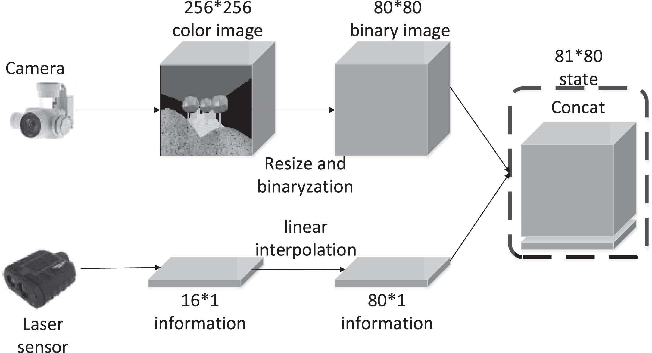
Get state for DQN.

Through the fitting ability of the convolutional neural network CNN, the 80*80 high-dimensional image input information is dimension-degraded, and the information in the image is extracted layer by layer using three-layer convolution: the pre-processed four consecutive moments of the visual sensor image are sequentially passed through the convolution kernels of 8*8*4, 4*4*32, and 3*3*64, and finally the feature map of the entire state is obtained.

Inspired by the Ada Boost [35] in the classifier algorithm, this paper proposes a Multi-Branch (MB) network structure. We improve the structure of the action-value network. The Nature DQN algorithm uses a single network to estimate the Q-value directly, while the Dueling DQN algorithm accelerates the convergence speed of DRL algorithm by separating action advantage A and state value V. Since the main purpose of action-value function calculation is to select the optimal Q-value for decision-making calculation, action advantage A is particularly important for the selection of the optimal strategy in the calculation of action-value. Using multiple action advantage branches to replace a single branch calculation can estimate the Q-value more accurately without redundant computation, as showing in the Fig. 3.

Fig. 3

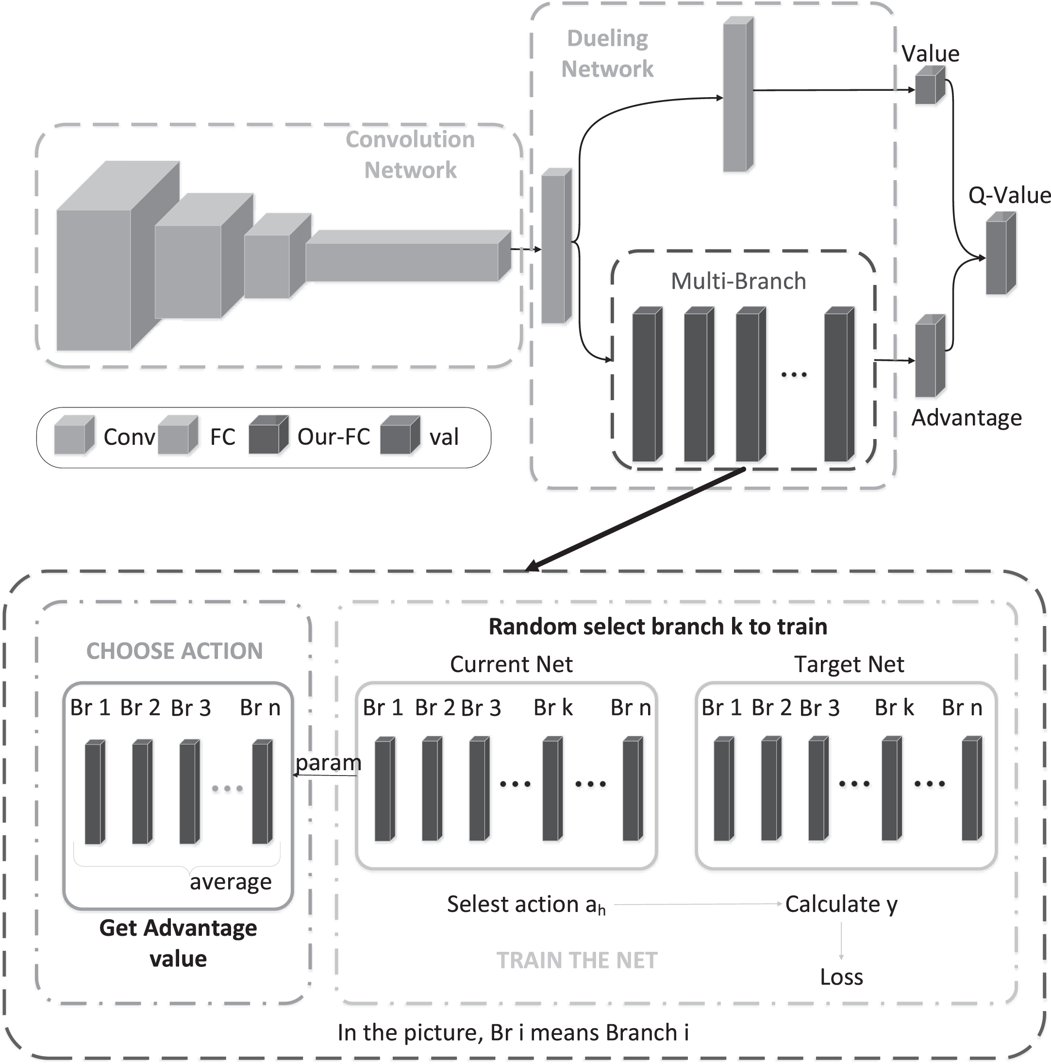
Multi-Branch Network.

In comparison with the original algorithm, three action advantage branches are used to estimate the action advantage A. The output of the i-th branch is A_i (s_t, a_t ; θ, α, β_i). Each time, the action selection is determined by the all branches’ output, not only by only one network branch. As show in Equations (6) and (7), the branches’ networks are slightly related in the training process. The training data of the three branches’ networks are all from the same sample database. In each training step, we randomly train one of the action advantage branches. While training one branch network, we use other advantage branches’ output as current branch’s tag action-value, which can separate the action evaluation and action selection, and solve the problem of over-estimation. As showing in Fig. 3 and Equation (8):

$\begin{matrix} Q_{i} (s_{t}, a_{t}; θ, α, β_{i}) = V (s_{t}; θ, α) \\ + A_{i} (s_{t}, a_{t}; θ, β_{i}) - \frac{1}{| A_{i} |} \sum_{a} A_{i} (s_{t}, a_{t}; θ, β_{i}) \end{matrix}$ (6) $Q (s_{t}, a_{t}; θ, α, β) = \frac{1}{N} \sum_{i = 0}^{N} Q_{i} (s_{t}, a_{t}; θ, α, β_{i})$ (7)

$\begin{matrix} y_{i} = r + γ \frac{1}{N - 1} \sum_{j \neq i}^{N} Q^{'} \\ (s_{t + 1}, \underset{a^{'}}{argmax} Q (s_{t + 1}, a^{'}, θ, β_{i}), θ^{'}, β_{j}^{'}) \end{matrix}$ (8)

On the one hand, using multi-branch action advantage networks to estimate the action-value can ensure that the algorithm will not shake violently. On the other hand, using this networks to estimate can ensure the accuracy of the action-value, reduce the possibility of poor selection of the action in the initial stage of training, and accelerate the network convergence rate.

3.3 Policy design

To solve the over-estimation problem, this paper proposes a Revise-Q Mechanism (RQ). Based on the original algorithm, the iterative calculation of the action-value function is improved. Because the main purpose of the action-value function calculation is to select the optimal Q-value for decision-making, whether the Q-value is accurate is not important. So we add a correction term to the calculation of tag value to correct the difference between the optimal value and the suboptimal value. It can reduce the suboptimal action-value without changing the optimal action-value function. Besides it can increase the difference between the optimal action-value and the suboptimal action-value, so as to not choose the suboptimal strategy in the action decision.

As suggesting above, the super parameter τ is added as the correction index. When the action u in experience sample data is same as the action selected in the current eval function based on current network parameter θ (ifu = argmaxQ (s_t+1, a′|θ)), it is considered that the action is the optimal action and does not need to be corrected, and the Q-value correction function is 1. Otherwise, it is considered that the action selected is the suboptimal action and its Q-value is higher than the optimal value due to overestimation. So, the current suboptimal value needs to be corrected. As showing as Equations (9) and (10). $RQ = {\begin{matrix} 1 \\ τ^{Q (s_{t}, a_{t} | θ^{'})} \end{matrix} \begin{matrix} if u = argmaxQ (s_{t + 1}, a^{'} | θ) \\ else \end{matrix}$ (9) $y = r + γ Q^{'} (s_{t + 1}, \underset{a^{'}}{argmax} Q (s_{t + 1}, a^{'}, θ), θ^{'}) * RQ$ (10)

The action u comes from the experience sample data. DQN only calculates and updates the Q-value corresponding to the selected action u in state s. However, due to the continuous updating of the network for the prediction and evaluation of the action-value, the action u in experience is not necessarily consistent with the action selected in the current network. In another word, the existence of bias estimation leads that the past agent cannot choose optimal action. Even through, the Q-value corresponding to the suboptimal action is reduced and the probability of each suboptimal action is reduced in every training update step. Through continuous updating, the agent can select the optimal strategy more stably and jump out of the sub-optimal strategy to reduce the impact of over-estimation on the network. The algorithm can better explore the optimal strategy. As showing the Fig. 4:

Fig. 4

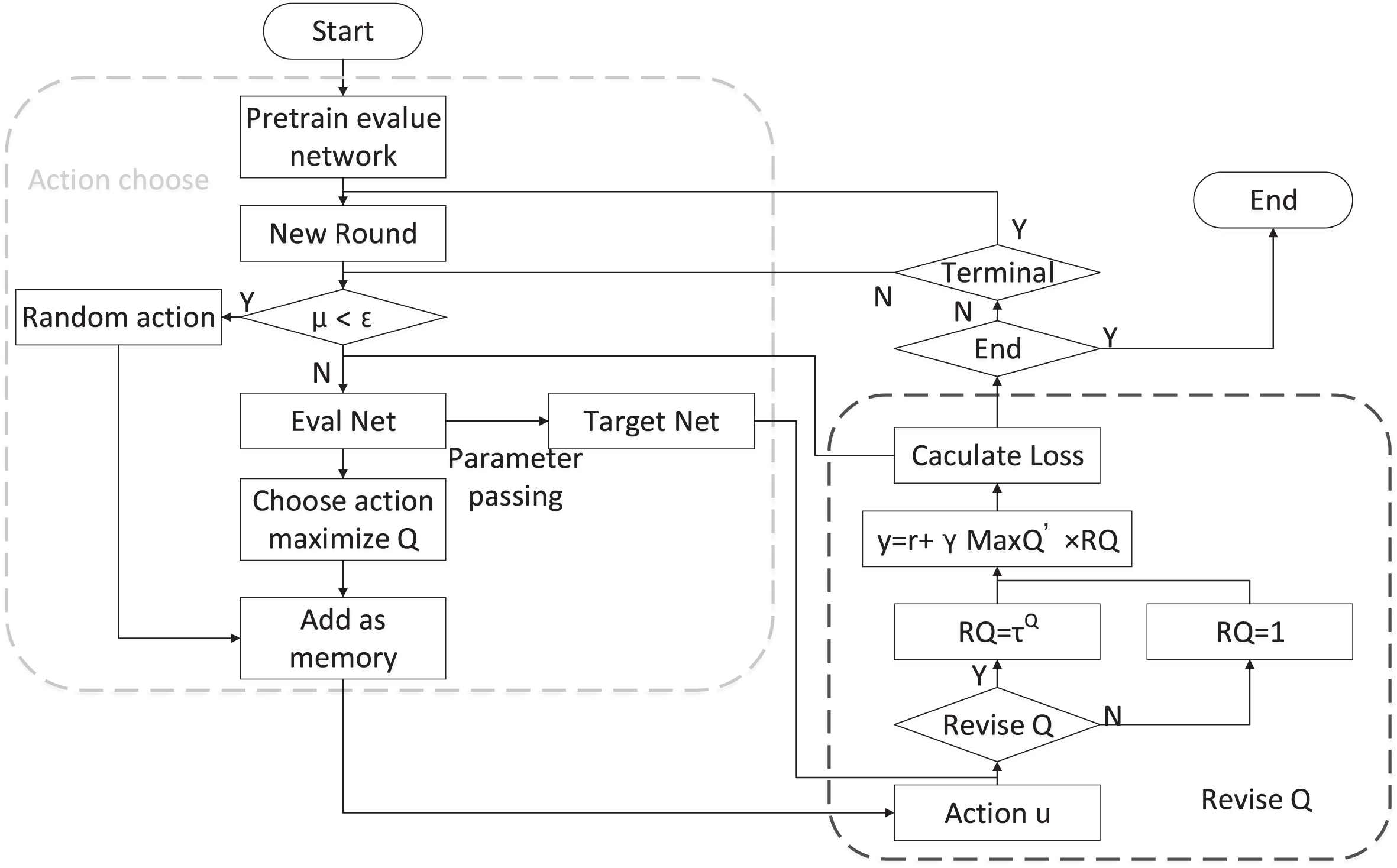
Revise-Q Algorithm.

4 Result analysis and evaluation

4.1 Experimental setting

4.1.1 Environment construction

Several scenes of obstacles suitable for UAV flight environment are built on the V-Rep simulation platform. Besides several kinds of common obstacles are set up between the starting point and the endpoint, such as tables, chairs, bookcases, people, windows, etc. Obstacle scenarios are divided into a training scenario(room1) and two test scenarios(room2, room3). The training scenario contain many types of obstacles. The test scenarios change the order of obstacles without changing obstacle categories. In the training scenario, the whole network is trained to obtain the optimal strategy and reach the final target point. Then, the trained model is used to test its obstacle avoidance ability in the test scenario without secondary training. As showing in the following Fig. 5.

Fig. 5

Obstacle avoidance scenarios.

There are many kinds of sensor used to avoid obstacles on drones. For example, GPS for obtaining the three-dimensional position and speed information, a gyroscope for monitoring the three-axis angular velocity of the drone, and a barometer for calculating the flying height etc. Different sensors can play different roles for different obstacle avoidance algorithms. In this paper, the IN-SIGHT series of visual sensor is used to obtain 256*256 picture information and a laser distance sensor to obtain 16*1 distance information. The combination of the front sensors information are used to avoid obstacles.

4.1.2 Action space

Due to UAV mobility and track restrictions, it is necessary to rationally discretize the entire UAV action space to obtain UAV decisive actions. We disperse the state space by the minimum turning radius (Rad_turn), available flying height(h), etc of the UAV.

According to the restriction of the UAV turning radius, the horizontal flight length is determined. We set the horizontal flight length of UAV according to Rad_turn to ensure the UAV have the highest maneuverability in the minimum state space. As showed in Fig. 6, black grids represent obstacles and white areas represent accessible areas.

Fig. 6

Action space.

To sum up, the continuous motion of the UAV is divided into nine actions. As showed in the Fig. 6. The UAV is in the position of the black block, and nine actions as showed in the light gray block are available.

4.1.3 Reward design

The Equation (11) shows several reward functions we set. The transfer distance reward r_dis is representing the difference between the D_tar-now and D_tar-start. D_tar-now is the euclidean distance between the target point and the current position and D_tar-start is the Euclidean distance between the starting point and the target point. The reward r_dis is aim to make the aircraft move toward the target position. The UAV flight height penalty reward r_h is to make the drone fly as close as possible to the cruising altitude h. The punishment reward of flight fuel consumption r_oil is set to ensure that the aircraft can avoid obstacles with lower fuel consumption. Besides, $w_{hor}^{oil}$ and $w_{ver}^{oil}$ respectively indicate the fuel consumption weights in the horizontal and vertical directions when different actions are taken, and dis_hor and dis_ver represent the distances that the aircraft moves in the horizontal and vertical directions for a single time step, respectively. Last, the terminal reward is set to give the agent a positive reward while reaching target or a negative reward while crashing. ${\begin{matrix} r_{dis} = D_{tar - start} - D_{tar - now} \\ r_{h} = | z_{now} - h | \\ r_{oil} = w_{hor}^{oil} {dis}_{hor} + w_{ver}^{oil} {dis}_{ver} \\ r_{terminal} = {\begin{matrix} + 1.5 \\ - 1.5 \end{matrix} \begin{matrix} reach target \\ crash \end{matrix} \end{matrix}$ (11)

The final reward function is Equation (12), where w_i is the weight value of the different reward functions: $r = {\begin{matrix} r_{terminal} \\ w_{0} * log (r_{dis}) + w_{1} * r_{h} + w_{2} * r_{oil} \end{matrix} \begin{matrix} terminal \\ else \end{matrix}$ (12)

4.2 Experimental parameters

The evaluation of the model path planning ability is carried out in the V-REP environment. The task of our model is to find the optimal sequence of actions from the starting point to the target point without collision. The model has a limited number of steps in each round, and the round ends early when the agent hits an obstacle or reaches the target. In order to verify that the model has ability to adapt to different environments, the experiment is divided into two groups. We train the model in the training scenario, and test in a training scenario and two testing scenarios. For each group RQ-Dueling-DQN (change policy), MD-Dueling-DQN (change network) compared by DQN, Dueling-DQN is employed to show the advantage of our idea.

To effectively compare the advantages and disadvantages of each algorithm, this paper uses the same set of parameters for different algorithms and uses the adaptive moment estimation optimization algorithm (Adam Optimizer) to control the learning rate, so that the learning of parameters is more stable. The policies and networks used in the experiments have been introduced in the previous chapter, Table 1 provides the parameters we used in the experiments.

Table 1
Summary of Algorithmic Parameters

Hyper-parameter Name Value Meaning

Minibatch 32 The number of sampled transition from Memory each step

N 300 Update frequency of the target network

Replay_Memory 5000 The number of previous transitions to remember

λ 0.99 The decay rate of past observations

α 3e-6 Learning rate

τ 0.95 Revise-Q parameter

Observe steps 200 The steps agent start to learn

Episode num 100 The number of episodes agent is trained

Episode steps 5000 Each Episode contains training steps

ɛ_init/ɛ_final 0.3/0.1 The probability agent randomly selected an action

Hyper-parameter Name	Value	Meaning
Minibatch	32	The number of sampled transition from Memory each step
N	300	Update frequency of the target network
Replay_Memory	5000	The number of previous transitions to remember
λ	0.99	The decay rate of past observations
α	3e-6	Learning rate
τ	0.95	Revise-Q parameter
Observe steps	200	The steps agent start to learn
Episode num	100	The number of episodes agent is trained
Episode steps	5000	Each Episode contains training steps
ɛ_init/ɛ_final	0.3/0.1	The probability agent randomly selected an action

The premise that the model ultimately achieves good training results is that the value evaluation network can accurately identify different obstacles. The training process include 100 episodes of train. Each episode consists of a training stage which contains 5000 training steps and a testing stage which contains a round of test. We record the test the test data of each episode to evaluate different algorithms.

To evaluate the performance of the model we define the following metrics:

Distance: the UAV flight distance in each round;

Reward: the average reward in the testing stage;

Finish-time: the number of rounds that successfully find the target point during the training process;

Q-Value: the average Q-Value in the testing stage;

Loss: the loss during training.

4.3 Test and result analysis

By training our method in training scenarios, we can evaluate the performance of the algorithm. Besides we record the distance traveled, the reward obtained, the number of times to reach the target point and finish the mission, the loss during training and the change of Q-value, as showed in Fig. 7. We use these data to analyze the advantages and disadvantages of the algorithm and the reasons for this situation.

Fig. 7

Algorithm training performance.

Figure 7(a) is the curve of flying distance and round number. Unlike the two-dimensional obstacle avoidance, the number of aircraft action in three-dimensional space is more than the vehicle of two-dimensional. Dueling-DQN divides the original action-value function into two branches, the action advantage function and the state value function and makes it possible to converge more quickly. The RQ improvement method has a low convergence speed in early training. This is because the agent is likely to choose an action at the beginning of training and misjudge it as the best action, which is actually a sub-optimal action. Due to the introduction of correction items, sub-optimal movements are gradually excluded in the training. But there are still other sub-optimal actions being trained because they have not been suppressed. So the convergence speed of RQ in the early training stage is low. However, the MD algorithm can converge quickly. Because the multi-branch network structure can calculate the Q-values by averaging multiple branch networks’ output, rather than relying on a single branch network to make decisions. At the same time, it can be guaranteed that the algorithm performance does not change too much due to the influence of a single network with some abnormal sample data.

Figure 7(b) shows the average return from test phase in every training episode. Some algorithms fluctuate greatly during the training process, and some have converged in the early stage but frequently oscillated in the late training period. It is because the neural network is over-fitted. Since the multi-branch network can estimate the action advantage A value more accurately, the MB algorithm can converge quickly. Accurate estimation also makes its stability slightly improved. Although the RQ convergence speed is low in the early training, its inhibitory effect on sub-optimal actions makes the algorithm find a better strategy in the later stage of training. While other algorithms converge to the local optimum and can’t find better strategies, the RQ algorithm can get the best strategy by suppressing sub-optimal actions. The RQ algorithm’s reward converged to a higher level than the others.

Figure 7(c) shows the finish time in every training episode. The low number of tasks completed by Dueling and Nature algorithms indicates that these two original algorithms can’t work well. And Finish-time rise rate drops to zero, showing that the algorithms have fallen into overfitting. After 30 episodes, the number of MB algorithm task completions has been rising at a steady rate. Although the Finish/Episode rate fluctuates, the algorithm basically converges. Due to the introduction of a correction factor, RQ mechanism uses extra computation to suppress sub-optimal actions. And the task of RQ algorithm was completed very late for the first time. But after its convergence, its finish rate can remain stable.

Figure 7(d) reflects the change of all actions’ Q-value. For the MB algorithm, multiple branch networks are trained separately. So the update direction of each branch network will be different, and the Q-value is lower than the original algorithm. The RQ algorithm reduces the coefficient of the sub-optimal actions’ action-value function. Therefore, the action value function of the sub-optimal action is smaller, resulting in the average value of the action value function of all actions is much smaller than the original algorithm.

Fig. 8

The test on the several scenes after training.

Figure 7(e) is the loss of algorithm in the training. For RL, the loss of training is not always reduced but fluctuates constantly. This is because the target function is constantly changing guided by the return function. However, from the analysis in the previous paragraph, we know that the Q-value of the improved algorithm is less than the original algorithm Q-value, so the loss is relatively small.

As showed in Fig. 8, we use the trained weight to test the performance in several scenarios without secondary training. Each algorithm can converge and avoid obstacles in the training and test scenarios. It proves the ability of the agent to avoid obstacles through the DRL algorithm. Among them, the obstacle avoidance strategy obtained by the RQ algorithm is obviously better than the other algorithms.

We test the agent in the above environment and record the reward obtained by the agent (Round average reward), the variance between each action (Variance Q-value), and the average value of each action (Average Q-value). As showed in Table 2, the MB-Dueling-DQN algorithm’s return value is slightly improved compared with the original algorithm. Besides, the improved RQ algorithm significantly enhances the superiority of the obstacle avoidance strategy by reducing the sub-optimal action function, and the average return of the round is increased by 25% . At the same time, the single-step Q-value variance of the RQ algorithm is significantly higher than other algorithms, which prove that the action-value of the optimal action is significantly higher than other sub-optimal actions. This ensures that the algorithm can select the optimal strategy for each step.

Table 2

Performance of various algorithms

Algorithm		Nature-DQN	Dueling-DQN	RQ-Dueling-DQN	MB-Dueling-DQN
Round	Room1	0.1246	0.1351	0.1622	0.1375
average	Room2	0.1235	0.1323	0.1621	0.1356
reward	Room3	0.1260	0.1318	0.1622	0.1340
Variance Q-value		0.1257	0.1246	0.6898	0.1297
Average Q-value		17.403	15.367	3.108	9.371

5 Conclusion

This paper develops an end-to-end deep reinforcement learning algorithm for UAV obstacle avoidance based on multi-sensor in complex environments. Besides, we propose two ways to solve the problem of overestimation of RL and make a reasonable analysis about algorithm performance.

For the training model network, the obstacle avoidance ability is tested in the test scenarios without secondary training to verify the feasibility of DRL to realize the obstacle avoidance of the drone.

Besides, for the problem of slow convergence caused by over-estimation, we create Multi-Branch (MB) dueling structure to estimate Q-value more accurately.

In addition, in the process of RL training, we add correction factors and adopt the improved Revise-Q (RQ) mechanism. In this way, the problem of selecting sub-optimal action caused by overestimation is solved. And it is easier to obtain the optimal solution.

In the end, simulation experiments have shown that our algorithm is much better than traditional DQN algorithms in terms of learning speed, stability and effect.

6 Future work

This paper conducts a detailed research on reinforcement learning UAV obstacle avoidance. However, the algorithm has only been studied by simulation and needs to be migrated to a real UAV for verification.

References

Akshya

and Priyadarsini

P.L.K.

, Graph-based path planning for intelligent UAVs in area coverage applications, Journal of Intelligent & Fuzzy Systems 6(39) (2020), 8191–8203.

Yong

, US military report: Unmanned Systems Roadmap, Defense Technology Journal 28(2) (2008), 2007–2032.

Lee

J.K.

, Kim

J.O.

and Park

S.J.

, A study on the UAV image-based efficiency improvement of bridge maintenance and inspection, Journal of Intelligent & Fuzzy Systems 2(36) (2019), 967–983.

Thampi

S.M.

, El-Alfy

E.M.

and Trajkovic

, Intelligent autonomous navigation system for UAV in randomly changing environmental conditions, Journal of Intelligent & Fuzzy Systems 5(38) (2020), 6619–6625.

Chai

, Savvaris

, Tsourdos

, Chai

and Xia

, A review of optimization techniques in spacecraft flight trajectory design, Progress in Aerospace Sciences 109 (2019), 100543.

Ragi

and Chong

E.K.P.

, UAV Path Planning in a Dynamic Environment via Partially Observable Markov Decision Process.

Choset

, Sensor-Based Exploration: The Hierarchical Generalized Voronoi Graph, International Journal of Robotics Research 19(2) (2001), 96–125.

Bhattacharya

and Gavrilova

M.L.

, Roadmap-Based Path Planning - Using the Voronoi Diagram for a Clearance-Based Shortest Path.

Roberge

, Tarbouchi

and Labonte

, Comparison of Parallel Genetic Algorithm and Particle Swarm Optimization for Real-Time UAV Path Planning, Ieee Transactions On Industrial Informatics 9(1) (2013), 132–141.

10.

, Ding

and Zhou

, Phase Angle-Encoded and Quantum-Behaved Particle Swarm Optimization Applied to Three-Dimensional Route Planning for UAV, IEEE Transactions on Systems Man & Cybernetics Part A 42(2) (2012), 511–526.

11.

, Wang

, Li

, Yao

, Huang

and Yang

, Path planning for solar-powered UAV in urban environment, Neurocomputing 275 (2018), 2055–2065.

12.

Yao

and Wang

, Dynamic Adaptive Ant Lion Optimizer applied to route planning for unmanned aerial vehicle, Soft Computing (2016).

13.

Zhang

and Duan

, Three-Dimensional Path Planning for Uninhabited Combat Aerial Vehicle Based on Predator-Prey Pigeon-Inspired Optimization in Dynamic Environment, IEEE/ACM Transactions on Computational Biology & Bioinformatics 14(1) (2017), 97–107.

14.

Khatib

, Proceedings. 1985 IEEE International Conference on Robotics and Automation (2003).

15.

Peng

, Wang

and Su

, UAV feasible path planning based on disturbed fluid and trajectory propagation, Chinese Journal of Aeronautics 28(4) (2015).

16.

, Wang

, Li

and Su

, Formation Obstacle Avoidance: A Fluid-Based Solution, Ieee Systems Journal 14(1) (2020), 1479–1490.

17.

Sutton

R.S.

and Barto

A.G.

, Reinforcement Learning, A Bradford Book 15(7) (1998), 665–685.

18.

, Engels

D.W.

and Sarma

S.E.

, International Symposium on Applications and the Internet Workshops (SAINTW’06), IEEE, Phoenix, AZ, USA (2006), 4–91.

19.

Chen

and Wei

, 2008 Fourth International Conference on Natural Computation, IEEE, Jinan, China (2008), 632–636.

20.

Volodymyr

, Koray

, David

, Andrei A

, Joel

, Marc G

, Alex

, Martin

, Andreas K

, Georg

, Stig

, Charles

, Amir

, Ioannis

, Helen

, Dharshan

, Daan

, Shane

and Demis

, Human-level control through deep reinforcement learning, Nature 518(7540) (2015), 529–533.

21.

Wang

, Schaul

, Hessel

, van Hasselt

, Lanctot

and de Freitas

, Dueling Network Architectures for Deep Reinforcement Learning, Computing Research Repository (2016), 1995–2003.

22.

van Hasselt

, Guez

and Silver

, Deep Reinforcement Learning with Double Q-learning, Computer Science (2015).

23.

Schaul

, Quan

, Antonoglou

and Silver

, the International Conference on Learning Representations 2016, San Juan, Puerto Rico (2016).

24.

Osband

, Blundell

, Pritzel

and Van Roy

, Deep Exploration via Bootstrapped DQN, in: Lee, D. D., Sugiyama, M., Luxburg, U.V., Guyon, I.,Garnett, R. (Eds.), Advances in Neural Information Processing Systems 29, Curran Associates, Inc. (2016), 4026–4034.

25.

Anschel

, Baram

and Shimkin

, 34th International Conference on Machine Learning, IEEE, Sydney, Australia (2017), 176–185.

26.

Narasimhan

, Kulkarni

and Barzilay

, Conference on Empirical Methods in Natural Language Processing 2015, Lisbon, Portugal (2015).

27.

Hausknecht

and Stone

, 2015 AAAI Fall Symposia, Arlington, Virginia, USA (2015).

28.

Lample

, Chaplot

D.S.

, 31st AAAI Conference on Artificial Intelligence (2016).pre

29.

Schulze

and Schulze

, Intelligent Systems Conference 2018, London, United Kingdom (2018).

30.

Chen

, Fengb

and Jialunb

, Controlling a cargo ship without human experience using deep Q-network, Journal of Intelligent & Fuzzy Systems 5(39) (2020), 7363–7379.

31.

, Yao

, Xiao

and Guo

, Intelligent controller for passivity-based biped robot using deep Q network, Journal of Intelligent & Fuzzy Systems 1(36) (2019), 731–745.

32.

Xie

, Meng

, Zhou

, Ma

and Wu

, Heuristic Q-learning based on experience replay for three-dimensional path planning of the unmanned aerial vehicle, Science Progress 103(1) (2019), 399520656.

33.

Wang

, Wang

and Zhang

, Deep-Reinforcement-Learning-Based Autonomous UAV Navigation With Sparse Rewards, Ieee Internet of Things Journal 7(7) (2020), 6180–6190.

34.

Bouhamed

, Ghazzai

, Besbes

and Massoud

, (2020).

35.

Cao

, Miao

, Liu

and Gao

, Advance and Prospects of AdaBoost Algorithm, Acta Automatica Sinica 39(6) (2013), 745–758.