Dual graph wavelet neural network for graph-based semi-supervised classification

Abstract

Vertex classification is an important graph mining technique and has important applications in fields such as social recommendation and e-Commerce recommendation. Existing classification methods fail to make full use of the graph topology to improve the classification performance. To alleviate it, we propose a Dual Graph Wavelet neural Network composed of two identical graph wavelet neural networks sharing network parameters. These two networks are integrated with a semi-supervised loss function and carry out supervised learning and unsupervised learning on two matrixes representing the graph topology extracted from the same graph dataset, respectively. One matrix embeds the local consistency information and the other the global consistency information. To reduce the computational complexity of the convolution operation of the graph wavelet neural network, we design an approximate scheme based on the first type Chebyshev polynomial. Experimental results show that the proposed network significantly outperforms the state-of-the-art approaches for vertex classification on all three benchmark datasets and the proposed approximation scheme is validated for datasets with low vertex average degree when the approximation order is small.

Keywords

Big graph mining vertex classification semi-supervised learning graph convolutional networks graph wavelet transform

1 Introduction

With the rapid popularity of social networks such as Facebook, Twitter, Weibo, and WeChat, a large amount of structured and semi-structured data are continuously being produced [1]. These data have huge commercial value and thus attract more and more researchers’ attention to graph mining [2]. As a representative of graph mining, the vertex classification problem studies how to infer labels of unlabeled vertices in a given graph with a small number of vertices labeled. Solutions to this problem have many applications in fields such as social network recommendation, e-Commerce recommendation, and sociological study of communities [3].

However, it is difficult, if not possible, to make high-quality predictions because the number of labeled samples in the dataset to be classified is much smaller than that of unlabeled ones [1]. There are many reasons. First, labeling data samples often requires human support and thus is expensive. For instance, item recommendation in e-Commerce often relies on users to score the product they bought, but no one want do this without reward [4]. Second, labeling data samples may threaten user’s privacy. For example, political affiliation prediction in a social network depends on users’ political views, but most are reluctant to share this sensitive information. Traditional supervised classification techniques such as the support vector machine [5] and k-nearest neighborhood [6] often rely on a large number of labeled samples to train and thus can not be applied to solve this problem.

Recently, researchers have proposed graph-based semi-supervised learning techniques by making use of graph topology information to improve the classification performance based on two essential assumptions. One is the local consistency that adjacent vertices are likely to have similar labels; the other one is the global consistency that vertices with the same context may have similar labels [7]. Existing graph-based semi-supervised learning methods can be classified into two categories: (1) graph-based regularization ones such as LP (Label propagation) [7]; and (2) graph embedding ones such as DeepWalk [8], LINE [9], and node2vector [10]. Deep Learning (DL) is a subset of Machine Learning that uses numerous layers of algorithms similarly to the way neurons are used in the human brain [11]. As DL techniques such as CNN and RNN have made breakthroughs in image recognition [12], video processing [13], and natural language processing [14], some researchers are trying to transplant them to irregular graphs. For example, Gori et al. [15] pioneered the research of graph neural networks and proposed the recursive graph neural network Gori GNN (Graph Neural Network) based on message passing and then various types of graph neural networks sprang up like bamboo shoot. The ones closely related to our work can be classified into two kinds: (1) spatial-based graph convolutional network such as GraphSage [16]; and (2) spectral-based graph convolutional networks such as Spectral GCN (Graph Convolutional Network) [17], ChebyNet [18], GCN [19], GWNN (Graph Wavelet Neural Network) [20], and DGCN (Dual Graph Convolutional Network) [1]. All these graph neural networks [1 , 15–20] extract vertex feature representations by stacking multiple hidden layers and fed them into the output layer to obtain the prediction results.

In summary, traditional supervised learning methods [5, 6] are not suitable to solve the vertex classification problem because the number of labeled vertices is limited; graph-based semi-supervised learning methods [7, 10] have multi-step pipelines and thus are hard to optimize; graph neural networks [15 –19] have poor classification accuracies as they do not make full use of unlabeled vertices; graph neural networks [1, 20] improve classification accuracies by introducing regularization terms that reflect sample distributions to objective functions of their output layers. Inspired by [1, 20], we propose a Dual Graph Wavelet Neural Network (DGWN) for the vertex classification problem. DGWN consists of two identical graph wavelet neural networks with shared network parameters. These two networks are integrated by a semi-supervised loss function and conduct supervised learning and unsupervised learning on two matrixes, respectively. These matrixes are extracted from the same graph dataset with different levels of consistency information embedded. Experimental results show that our proposed network outperforms state-of-the-art classification methods on all three benchmark datasets. The main contributions of this work are as follows:

We propose a dual graph wavelet neural network composed of two identical graph wavelet neural network sharing network parameters. This design combines the advantages of supervised learning and unsupervised learning to improve the classification accuracy.

We design an algorithm to construct the Positive Pointwise Mutual Information (PPMI) matrix from the raw graph dataset based on the random walk and random sampling. The PPMI matrix embeds the global consistency information of the graph.

We define the graph convolutional operation by using the graph wavelet transform. The sparsity of graph wavelets makes it much more computational efficient; the locality of graph wavelets makes the proposed DGWN have a good classification performance.

We present an approximate scheme to calculate the bases of the graph wavelet transform and its inverse based on the Chebyshev polynomial. It can significantly reduce the complexity of the proposed network with tolerable performance degradation.

The rest of this work is organized as follows: Section 2 formulates the vertex classification problem; Section 3 introduces the detailed design of the proposed DGWN; Section 4 analyzes the parameter complexity of the proposed network and presents an approximate scheme for calculating the bases of the graph wavelet transform and its inverse; Section 5 validates the performance of the proposed network through a series of experiments; Section 6 reviews the related work on the vertex classification problem; Section 7 concludes this work.

2 Graph-based Semi-supervised Classification Problem

2.1 Graph data modeling

Data generated from social network platforms can naturally be represented as graphs. They can be weighted or unweighted, directed or undirected, connected or disconnected. In this work, we assume that the graph is weighted and undirected and denote it as $G$ =(V, E, A), where V = {v₁, v₂, . . . , v_n} and E ={e_ij|v_i, v_j∈ V } are the set of vertices and edges, respectively; and A is the adjacent matrix with element a_ij representing the weight of edge e_ij. Each vertex v_i ∈ V has d attributes and all attributes of all vertices form the vertex feature matrix X ∈ R^n×d. Every column vector x = {x₁, x₂, . . . , x_d}∈R^d of X is a graph signal with x_i denoting the values of the i^th attribute of all vertices. In addition, a small number of vertices in the graph have labels. We denote the labeled and unlabeled vertex sets as V_L and V_U, respectively, where V_L ∪ V_U = V, V_L∩ V_U = Ø, and |V_L| ⪡ |V_U|. ∀v ∈ V_L, we denote its label as y ∈ { 0, 1 } ^|C| with C be the set of all possible labels.

2.2 Problem formulation

Given an undirected weighted graph $G = (V, E, A)$ with a small subset V_L of labeled vertices, the vertex classification problem is to infer the label y ∈ { 0, 1 } ^|C| of each unlabeled vertex v ∈ V_U. Note that some researchers assume that labels of labeled vertices are changeable during the inference process and then the goal is to predict labels of all vertices. We do not make this assumption in this work. The above problem can be modeled as a graph-based semi-supervised learning problem, the key to which is the consistency assumption. Often there are two consistency assumptions. One is the local consistency assumption that adjacent vertices may have the same label and the other one is the global consistency assumption that the vertices with the same context may have the same label. Assume that the loss functions of semi-supervised, supervised, and unsupervised learning are denoted as $L, L_{S}$ , and $L_{U}$ , respectively, then we have: $L = L_{S} + α L_{U}$ (1) where α∈ (0, 1) is a dynamic weighting factor; the design of $L_{S}$ and $L_{U}$ are closely related to the specific classifier. They will be discussed in Section 3.5.

2.3 Traditional classification method

We introduce the fundamental of the spectral-based GCN, which lays foundations for our proposed DGWN presented in Section 3. The core operation of the spectral-based GCN is the spectral graph convolution. It is defined in the Fourier domain through computing the eigendecomposition of the graph Laplacian matrix [21]. For a graph signal x ∈ Rⁿ defined on graph $G = (V, E, A)$ , the graph Fourier transform and its inverse of this signal are defined as $\hat{x} = U^{T} x$ and $x = U \hat{x}$ , respectively, where U = ( u ₁, u ₂, …, u _n) are the eigenvectors of the graph Laplacian matrix. Then we can define the graph convolutional operation *_G as: $x *_{G} y = U ((U^{T} x) ⊙ (U^{T} y)) = Ug (Λ) U^{T} x,$ (2) where ⊙ is the Hadamard product and g (Λ) is a diagonal matrix with Λ = {λ₁, λ₂, …, λ_n} being the corresponding eigenvalues of U. Often a spectral-based GCN learns embedding representations of vertices by stacking multiple graph convolutional layers and feeds them into the output layer to predict their labels.

2.4 Evaluation metrics

We establish a set of evaluation metrics including accuracy ac, precision pr, recall rate rc, and F1 score, to evaluate the performance of classifiers. Assume that (1) the graph dataset $G_{test} = (V_{test}, E_{test}, A_{test}$ ) for testing has |C_test| labels; and (2) the ratio of the number of vertices with label c_i (c_i ∈ C_test) to the number of all vertices is denoted as γ_i ∈ (0, 1), which satisfies ∑_{c_i∈c_test} γ_i = 1. Regarding each category as positive and the rest as negative, we can define the above four evaluation metrics as follows: (1) accuracy ac measures how many observations are correctly classified. It can be computed as $ac = \sum_{c_{i} \in C_{test}} γ_{i} * \frac{{TP}_{i} + {TN}_{i}}{{TP}_{i} + {TN}_{i} + {FP}_{i} + {FN}_{i}} = \sum_{c_{i} \in C_{test}} γ_{i} * \frac{{TP}_{i} + {TN}_{i}}{| V_{T} |}$ , where TP_i, TN_i, FP_i, FN_i represent the number of true positives, true negatives, false positives, and false negatives, respectively. (2) precision pr measures how many observations predicted as positive are actually positive. It can be computed as $pr = \sum_{c_{i} \in C_{test}} γ_{i} * \frac{{TP}_{i}}{{TP}_{i} + {FP}_{i}}$ . (3) recall rate rc measures how many observations out of all positive observations have we classified as positive. $rc = \sum_{c_{i} \in C_{test}} γ_{i} * \frac{{TP}_{i}}{{TP}_{i} + {FN}_{i}}$ . (4) F1 score is the harmonic mean between precision and recall and can be calculated as $F 1 = \frac{2 * pr * rc}{pr + rc}$ .

3 Graph-based Semi-supervised Classification Problem

3.1 An overview of the DGWN

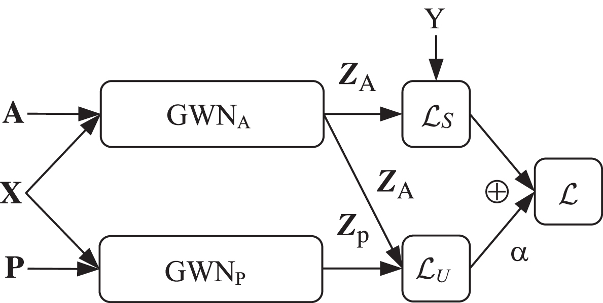
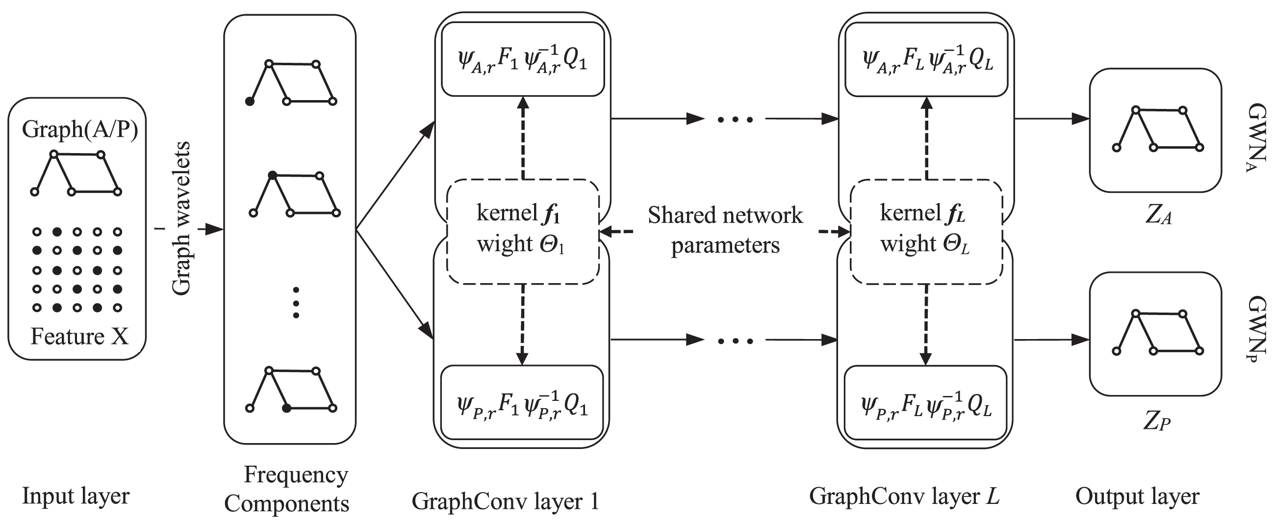
We can see from Figs. 1 2 that the proposed DGWN is composed of two identical graph wavelet neural networks GWN_A and GWN_P sharing network parameters. Each GWN is composed of an input layer, L graph convolutional layers, and an output layer, the principle of which will be presented in Section 3.2, 3.3, and 3.4, respectively. For GWN_A, it takes as input the adjacency matrix A embedding the local consistency information of the graph, the vertex feature matrix X , and label matrix Y to conduct supervised learning and output the label prediction matrix Z _A. For GWN_P, it takes as input the PPMI matrix P embedding the global consistency information of the graph and X to conduct unsupervised learning and output the label prediction matrix Z_P. The semi-supervised loss function that integrates these two networks is a weighted sum of the supervised learning loss and unsupervised learning loss, the definitions of which will be introduced in Section 3.5.

Fig. 1

An overview of the architecture of the proposed DGWN.

Fig. 2

The detailed structure of the proposed DGWN.

Table 7

Algorithm 1 (Vertex-context Co-occurrence Count, VCC)
Input: graph adjacent matrix A ∈ R^n×n; path length u; window size s; number of walks per vertex m;
Output: vertex co-occurrence count matrix O
1: VCC()¹
2: { O _ij ← 0, i, j ∈ [1, n] //Initialize O with zeros
3: Ω← Ø;
4: foreach vertexv_i ∈ Vdo
5: { foriter in rangedo
6: { π_i← RandomWalk (A, v_i, u) ; //obtain a path with v_i as the path root according to Equation (6)
7: Ω← uniform_pair_sampling (π_i, s);
8: for each pair (v_j, v_k) ∈ Ωdo
9: O _jk ← O _jk + b, O _kj ← O _kj + b;
10: }
11: }
12: }
13: }

3.2 Graph wavelet transform and graph convolution

In this section, we introduce the graph convolutional operation based on the graph wavelet transform. As GWN_A and GWN_P have the same structure, unless stated otherwise, we do not distinguish them in the rest of this section. Assume that Ψ _r={ψ_r1, ψ_r2, … , ψ_rn } is a basis of the graph wavelet transform. ψ_ri represents an energy signal diffusing from vertex v_i. It describes the local neighborhood structure of v_i with r being a scaling factor. Ψ _r can be computed as Ψ _r = UG _r U ^T, where U is the graph Fourier transform basis and $G_{r} = diag ({g (r λ_{i})}_{i = 1}^{n}$ ) is a scaling matrix with g (rλ_i)=e^λ_ir. Using the graph Fourier transform introduced in Section 2.3 for reference, we can define the graph wavelet transform and its inverse of a graph signal x as $\hat{x} = Ψ_{r}^{- 1} x$ and $x = Ψ_{r} \hat{x}$ , respectively, where $ψ_{r}^{- 1}$ =UG_-rU^T and G_-r is obtained by replacing rλ_i with-rλ_i. Then the graph convolutional operation *_G based on the graph wavelet transform can be obtained by substituting the graph wavelet transform basis Ψ_r for the graph Fourier transform basis U in Equation (2): $x *_{G} y = Ψ_{r} ((Ψ_{r}^{- 1} x) ⊙ (Ψ_{r}^{- 1} y)) = Ψ_{r} g_{θ} (Λ) Ψ_{r}^{- 1} x,$ (3) where g_θ (Λ) is computed by diagonalizing the spectral graph wavelet-kernel $\hat{g} = [g (λ_{1}), g (λ_{2}), \dots, g (λ_{n})]^{T}$ . To reduce the network parameter complexity, we break down the graph convolutional operation of the l^th layer (1≤l≤L) into two parts, feature transformation and graph convolution [20]. They are defined as: $Q_{l} = H_{l} Θ_{l}^{T}$ (4) $H_{l + 1} = σ (Ψ_{r} F_{l} Ψ_{r}^{- 1} Q_{l})$ (5) where Θ_l is the feature transformation matrix of the l^th layer; H_l and H_l+1 are the input and output of the l^th graph convolution layer; F_l is the diagonal matrix obtained by diagonalizing the spectral graph wavelet-kernel f _l = (f_l1, f_l2, …, f_ln) of the l^th layer.

3.3 Construction of graph topology representation matrix

The most commonly used graph topology representation matrix is the adjacency matrix A ∈ R^n ×n. It encodes the local consistency information of the graph, that is, the labels of two adjacent vertices may be the same. For the global consistency information, we use the positive pointwise mutual information matrix P ∈ R^n×n to embed it. The row vector p _i,: is the embedded representation of the vertex v_i; the column vector p_:,j is the embedded representation of the context ct_j ; p_ij represents the probability that the vertex v_i appears in the context ct_j. The matrix P can be obtained by random walk on the graph. Assume that the context ct_j of the vertex v_j is represented as a path π_j with v_j being the root node and a length of u, we can calculate p_ij as the frequency at which the vertex v_i appears on the path π_j. Suppose that the vertex index where a random walker locates at time τ is denoted as x (τ) and x (τ) = v_i, then the probability t_ij of the random walker walking to its neighbor vertex v_j at time τ + 1 is: $t_{ij} = pr (x (τ + 1) = v_{j} | x (τ) = v_{i}) = A_{ij} / Σ_{j} A_{ij}$ (6)

Performing random walk of length u on each vertex of the graph according to Equation (6) generates the path π representing the context of the vertex. Then vertex-context co-occurrence matrix O can be obtained by calculating the number of co-occurrences of any two vertices on each path by using the random sampling. ∀o_ij ∈ O, it represents the number of times that the vertex v_i appears in the context ct_j and can be used to calculate p_ij. Algorithm 1 gives a pseudo-code of obtaining the vertex-context co-occurrence matrix.

Theorem 1. The time complexity of Algorithm 1 is O (nmu²).

Proof. Algorithm 1 includes triple nested for-loops, which requires n, m, and u² iterations, respectively. Thus, the time complexity of Algorithm 1 is O (nmu²). Proofed.

Based on the vertex co-occurrence matrix O , we can calculate the co-occurrence probability of the vertex and the context and the corresponding marginal probabilities. Assume that these three probabilities are denoted as pr (v_i, ctj) , pr (v_i) and pr (ct_j), then we have: ${\begin{matrix} \begin{matrix} pr (v_{i}, {ct}_{j}) = O_{ij} / \sum_{i, j} O_{ij} \\ pr (v_{i}) = \sum_{j} O_{ij} / \sum_{i, j} O_{ij} \end{matrix} \\ pr ({ct}_{j}) = \sum_{i} O_{ij} / \sum_{i, j} O_{ij} \end{matrix}$ (7)

According to Equation (7), the value of p_ij of the positive point-by-point mutual information matrix P can be obtained by the following equation: $p_{ij} = \max (log (pr (v_{i}, {ct}_{j}) / (pr (v_{i}) pr ({ct}_{j})), 0),$ (8)

Algorithm 2 DGWN)
Input: vertex feature matrix X ∈ R ^n×d; graph topology matrix A ∈ R ^n×n and P ∈ R ^n×n; the indices of training data
for masking Y _L; dynamic weight function α (t); the number of graph convolution layer L;
Output: the trained model including feature transformation matrix Θ _l; spectral attention weights f _l
1: DGWN()
2: { forl in range [0, L] do
3: Randomly_initialize( Θ _l), Randomly_initialize( W _l), Randomly_initialize(f_l),
4: fort in range [0, num_of_epochs] do
5: { for each graph convolution layer l in range [0, L] do
6: { $H_{l + 1}^{A} \leftarrow h (ψ_{A, r}, ψ_{A, r}^{- 1}, F_{l}, Θ_{l}, H_{l}^{A})$ ;//Calculate output of layer l according to Equations (4) and (5)
7: $H_{l + 1}^{P} \leftarrow h (Ψ_{P, r}, ψ_{P, r}^{- 1}, F_{l}, Θ_{l}, H_{l}^{P})$ ; //Calculate output of layer l according to Equations (4) and (5)
8: }
9: $Z^{A} \leftarrow softmax (H_{L}^{A})$ ;
10: $Z^{P} \leftarrow softmax (H_{L}^{P})$ ;
11: Λ ← Λ _s + αΛ_U;
12: Θ _l, W _l, f _l← Adam_updating( Λ , Θ _l, W_l, f _l);
13: ifconvergedthen
14: break;
15: }
16: }

3.4 The vertex classification layer

We select the softmax function to define the output layer of the GWN. The function takes as input the output of the L^th graph convolution layer and outputs the predicted label of each unlabeled vertex: $Z = softmax (σ (Ψ_{r} F_{L} Ψ_{r}^{- 1} Q_{L}))$ (9) where $softmax (x_{i}) = \frac{exp (x_{i})}{\sum_{i} exp (x_{i})}$ and Z is an n * |C| dimensional matrix representing the prediction result with each column vector Z_j denoting the probability of all vertices having label c_j (c_j∈C). Because the difference between Z_A of GWN_A and Z_P of GWN_P is negligible at the end of neural network training, we may as well take Z_A as the output of the entire neural network.

3.5 The semi-supervised loss function

The two graph wavelet neural networks GWN_A and GWN_P are integrated by a semi-supervised loss function, which is defined as the dynamic weighted sum of supervised learning loss $L_{S}$ of GWN_A and unsupervised learning loss $L_{U}$ of GWN_P. For $L_{S}$ , we define it according to the cross-entropy as:

$\begin{matrix} L_{S} = \sum_{v_{i} ɛ V_{L}} l (y_{i}, Ψ_{i}) \\ = - \sum_{i ɛ V_{L}} \sum_{j = 1}^{C} Y_{ij} ln (Z_{T} (i, j)) \end{matrix}$ (10)

For $L_{U}$ , we define it as follows to ensure GWN_A and GWN_P output consistent prediction results by minimizing the difference between Z_A and Z_P as much as possible: $L_{U} = \sum_{v_{i}, v_{j} ɛ V_{U}} A_{ij} {| | Z_{A} (i, j) - Z_{P} (i, j) | |}^{2}$ (11)

The cross-entropy-based unsupervised loss function defined in Equation (11) can be regarded as training Z_P and Z_A by interpreting Z_A as a posterior distribution over |C| labels when GWN_A is trained. Then we can obtain the loss function of DGWN by combining Equations (1), (10), and (11): $\begin{matrix} L = L_{S} + α (τ) L_{U} = - \sum_{v_{i} ɛ V_{L}} \sum_{j = 1}^{c} Y_{ij} ln (Z_{ij}) \\ + α (τ) \sum_{i ɛ V} \sum_{j ɛ c} A_{ij} {| | Z_{A} (i, j) - Z_{P} (i, j) | |}^{2} \end{matrix}$ (12) where α (τ) is a temporal function of training step τ for. dynamically adjusting the relative importance of supervised and unsupervised learning at different stages. In the beginning, $L$ is dominated by the supervised learning loss. As the training process proceeds, increasing α (τ) along with τ will force the proposed DGWN to consider the knowledge learned by GWN_A on unlabeled samples.

3.6 DGWN training algorithm

The proposed DGWN is composed of two graph wavelet neural networks. They are in fact feed-forward neural networks and thus can be trained by using gradient descent methods such as the Batch Gradient Descent (BGD) and Stochastic Gradient Descent (SGD). As BGD has good convergence, we design an algorithm based on it to train our proposed network. Algorithm 2 presents the pseudo-code of our proposed training algorithm.

4 Theoretical analysis and optimization

4.1 Network complexity analysis

Theorem 2. The parameter complexity of the lth graph convolution layer of the DGWN is O (n + p_l × p_l+1).

Proof. Based on the definition of DGWN in Section 3, the l^th (1 ≤ l ≤ L) graph convolution layer of each GWN contains n + p_l × p_l+1 parameters, where n is the total number of vertices of $G$ and p_l is the number of features of each graph vertex has on the l^th layers. As GWN_A and GWN_P share network parameters, parameter complexity of the l^th layer of DGWN is O (n + p_l × p_l+1).

4.2 Approximation scheme for the graph wavelet transform

Calculating the bases of the graph wavelet transform and its inverse involve costly matrix eigendecomposition, the time overhead of which is unbearable for big graphs. To alleviate it, Hammond et al. [22] approximated ψ_r and $Ψ_{r}^{- 1}$ by using the first type Chebyshev polynomial. Its specific process is as follows:

The first type Chebyshev polynomial is defined as a set of orthogonal polynomials: T_k ( x ) =2xT_k−1 (x) − T_k−2 (x), where T₀ = 1 and T₁ = x. ∀x ∈ [–1, 1] , T_k (x) = cos (karccos (x)) and T_k (x) ∈ [–1, 1]. For each real-valued function h in a square-integrable Hilbert space $L^{2} ([- 1, 1], \frac{dx}{\sqrt{1 - x^{2}}}$ ), we can construct a uniformly convergent Chebyshev series $h (x) = \frac{1}{2} c_{0} + \sum_{k = 1}^{\infty} c_{k} T_{k} (x)$ with Chebyshev coefficients $c_{k} = \overset{2}{-} \int_{- 1}^{1} \frac{T_{k} (x) h (x)}{\sqrt{1 - x^{2}}} dx = \overset{2}{-} \int_{- 1}^{1} cos (k θ) h (\cos (θ)) d θ$ . ∀x ∈ [0, λ_max], the Chebyshev polynomials can be transformed to $T_{k}^{'} (x) = T_{k} (\frac{x - a}{a})$ with the help of domain shifting by using the transformation x = a(y + 1), where $a = \frac{1}{2} λ_{\max}$ and $\frac{x - a}{x} \in$ [–1,1]. Then we can approximate g (rx) as $g (rx) = \frac{1}{2} c_{0} + \sum_{k = 1}^{\infty} c_{k} T_{k}^{'} (x)$ , where x ∈ [0, λ_max] and $c_{k} = \int_{- 1}^{1} cos (k θ) g (ra (cos (θ) + 1) d θ$ . Truncating this Chebyshev expansion to K terms can obtain the approximation of the graph wavelet transform of graph signal x ∈ Rⁿ: $ψ_{r}^{- 1} x = \frac{1}{2} x + \sum_{k = 1}^{K} c_{k} T_{k}^{'} (L) x,$ (13) where $T_{k}^{'} (L) x$ can be efficiently computed according to $T_{k}^{'} (L) x = \frac{2}{a} (L - I) (T_{k - 1}^{'} (L) x - T_{k - 2}^{'} s (L) x)$ without matrix eigendecomposition.

5 Evaluation results

5.1 Experiment setup

(1) Dataset. The Citeseer dataset contains 3327 scientific publications and 4732 citation links between them. Publications and their citations form a citation network, where publications are divided into six categories and each of them is encoded by using the one-hot encoding scheme. The Cora dataset contains 2708 scientific publications and 5429 citation links between them. In its citation network, all the publications are divided into three categories and every publication is also encoded by using the one-hot encoding scheme. The Pubmed dataset contains 19,717 scientific publications and 44,338 citation links between them. In its citation network, all the publications are divided into three categories and every publication is encoded by a Term Frequency-Inverse Document Frequency (TF-IDF) vector derived from a dictionary consisting of 500 terms. Their detailed information is summarized in Table 1, where the label rate represents the proportion of labeled vertices for training.

Table 1
Graph Datasets Summary

Dataset #Vertices #Features #Edges Average vertex degree #Classes Label rate

Citeseer 3327 3703 4732 2.84 6 0.036

Cora 2708 1433 5429 4.01 7 0.052

Pubmed 19717 500 44338 4.50 3 0.003

Dataset	#Vertices	#Features	#Edges	Average vertex degree	#Classes	Label rate
Citeseer	3327	3703	4732	2.84	6	0.036
Cora	2708	1433	5429	4.01	7	0.052
Pubmed	19717	500	44338	4.50	3	0.003

(2) Baselines. To validate the performance of our proposed network, we select several state-of-the-art baselines with public source codes for comparisons. Their brief introductions are as follows:

DeepWalk regards a path generated by random walk on a graph as a “sentence” and applies the word sequence modeling technology in natural language processing to the path to obtain the vertex embedding. The source code of DeepWalk is publicly available 1 . LP [7] regards the vertex classification as the propagation of labels from labeled vertices to unlabeled ones on a graph. It is simple and easy to implement. Planetoid. Inspired by the Skip-Gram model [23],

PLANETOID [24] embeds graph topology and label information by using the positive and negative samplings. The source code of PLANETOID is publicly available 2 . Spectral CNN [17] defines the graph convolutional operation based on the graph Fourier transform to obtain embeddings of all vertices. ChebyNet [18] defines the graph convolutional operation by using K-order polynomial to obtain the embeddings of all vertices. The source code of ChebyNet is publicly available 3 . GCN [19] simplifies the ChebyNet network by using a first-order polynomial to define the graph convolutional operation. The source code of GCN is publicly available 4 . GWNN [20] defines graph convolutional operation by using the graph wavelet transform to obtain the embeddings of all vertices. The source code of GWCN is publicly available 5 . DGCN [1] consists of two GCNs sharing parameters. The source code of DGCN is publicly available 6 .

(3) Platform. The model of our hardware server is Inspur NF5280M5. It has two Intel Xeon Platinum 8270 processors, 754GB memory, 26TB hard drives, and four NVIDIA Tesla V100 GPUs. Its operating system is CentOS Linux 7.8.2003 and the compiler is GCC 4.8.5-44.

We implement the proposed DGWN by using Theano 1.0.4 7 and use the Xavier parameter initialization method proposed by Glorot and Bengio [25] to initialize network parameters including Θ_l and f _l. We trained and optimized the network by using Algorithm 2. In addition, we adopt the dropout method proposed by Srivastava et al. [26] to avoid over-fitting.

We establish a DGWN composed of two graph convolutional layers and train it on the aforementioned three graph datasets. They are partitioned into a training dataset, a test dataset, and a validation dataset by using the partitioning method proposed by Kipf and Welling [19]. The training process is terminated when the verification loss does not decrease for 50 consecutive epochs.

5.2 Experiments and result analysis

Experiment 1 (Classification Accuracy Validation) This experiment is designed to validate classification accuracy of the proposed network on different datasets. Best results are reported and the value of hyper-parameters on different datasets obtaining the best results are shown in Table 2. For comparisons, we implement the aforementioned nine classification methods and record their best results. Experimental results are shown in Table 3.

Table 2
Optimal values of hyper-parameters on different datasets

Dataset Citeseer Cora Pubmed

Hidden size 128 64 16

Learning rate 0.1 0.8 1

Dropout rate 0.5 0.9 0.1

Scale 0.5 1 2

Dataset	Citeseer	Cora	Pubmed
Hidden size	128	64	16
Learning rate	0.1	0.8	1
Dropout rate	0.5	0.9	0.1
Scale	0.5	1	2

Table 3

Comparisons of vertex classification accuracy of different methods

Method	Citeseer	Cora	Pubmed
DeepWalk [8]	43.2%	67.2%	65.3%
LP [7]	45.3%	68.0%	63.0%
Planetoid [24]	64.7%	75.7%	77.2%
Spectral CNN [17]	58.9%	73.3%	73.9%
ChebyNet [18]	69.8%	81.2%	74.4%
GCN [19]	70.3%	81.5%	79.0%
GWNN [20]	71.7%	82.8%	79.1%
DGCN [1]	72.6%	83.5%	80.0%
DGWN(ours)	75.3%	84.1%	81.2%

We can see from Table 3 that our proposed DGWN performs the best on all three datasets. DeepWalk and LP perform poorly on all three datasets, which agrees with the view mentioned in Section 1 that “graph-based semi-supervised learning methods have low classification accuracies”. Compared with PLANETOID, Spectral CNN performs better on all three datasets although they use similar sampling strategies to embed both the graph topology and label information. One possible reason is that the sampling strategy used by PLANETOID is too simple to fully embed all the known information. However, Spectral CNN performs worse than ChebyNet and GCN because the graph convolutional operation in Spectral CNN does not well meet the consistency assumption. GWNN improves classification accuracy over GCN by replacing the graph Fourier transform in GCN with the graph wavelet transform. DGCN is the-state-of the-art and achieves the highest classification accuracy on all three datasets by using a dual neural network architecture that integrates two GCNs with a semi-supervised loss function. This design enables DGCN consider the global consistency information for each vertex. Compared with DGCN, our proposed DGWN improves the classification accuracies on three datasets by 2.70%, 0.60%, and 1.20% respectively, by replacing the GCNs in DGCN with GWNs. There may be two reasons: (1) the basis of the graph wavelet transform better meets the locality assumption than that of the graph Fourier transform; and (2) the scaling parameter can adjust diffusion ranges of graph signals to best describe each vertex’s neighborhood or context.

Experiment 2 (Influence of network hyper-parameters on classification accuracy) This experiment is designed to study the influence of network hyper-parameters on classification accuracy. Hyper-parameters considered include the learning rate, the dropout rate, the scale parameter, and the hidden layer size. For each hyper-parameter, we vary it from a list of typical values and record the corresponding classification results on Cora with the other hyper-parameters set to the optimal values shown in Table 2. Experimental results are shown in Table 4.

Table 4

Influence of network hyper-parameters on the classification accuracy

(a) Hidden size
hiddenSize	Classification Accuracy
16	78.1%
32	81.0%
64	84.1%
128	83.4%
256	82.1%
(b) Dropout rate
DropoutRate	Classification Accuracy
0.10	69.7%
0.20	66.9%
0.30	61.3%
0.40	70.5%
0.50	65.2%
0.60	65.2%
0.70	82.4%
0.80	80.1%
0.90	84.1%
(c) Learning rate
LearningRate	Classification Accuracy
0.10	78.6%
0.20	83.5%
0.30	83.7%
0.40	82.3%
0.50	82.9%
0.60	83.7%
0.70	82.9%
0.80	84.1%
0.90	82.3%
1	82.8%
(d) Scale
Scale	Classification Accuracy
0.10	31.8%
0.20	57.2%
0.30	54.2%
0.40	78.4%
0.50	81.1%
0.60	83.3%
0.70	83.8%
0.80	83.3%
0.90	82.4%
1.00	84.1%

We can see from Table 4 that the scale parameter of the wavelet function has the biggest impact on the accuracy of the network vertex classification, followed by the dropout rate, the hidden layer size, and the learning rate. This is because that the Mean Squared Errors (MSEs) of the classification accuracies of the four hyper-parameters are 0.000211, 0.000788, 0.000148, and 0.001710, respectively. In addition, we find that classification accuracy is not a monotonic function of any hyper-parameter. Taking the hidden layer size hyper-parameter for example, the classification accuracy increases from 78.1%when hidden layer size is 16 to 84.1%when hidden layer size is 64 and then drops rapidly. For the other hyper-parameters, larger values are recommended.

Experiment 3: (Performance of the Chebyshev polynomial approximation scheme) This experiment is designed to validate the time efficiency of the Chebyshev polynomial approximation scheme and to study its influence on classification accuracy. We compare the mean training time per epoch of the original DGWN and DGWN using K-order Chebyshev polynomial as its propagation rule (denoted as DGWN-Cheby-K) over 300 epochs on different datasets and record their best classification accuracies. Experimental results are shown in Tables 5 6.

Table 5

Comparison of the time efficiency of different propagation models

Time (s/epoch)	Citeseer	Cora	Pubmed
DGWN	1.718	2.979	1710.131
DGWN-Cheby-K(K = 2)	2.237	1.906	256.040
DGWN-Cheby-K(K = 3)	3.411	4.626	1013.290
DGWN-Cheby-K(K = 4)	3.264	5.538	3845.382

Table 6

Classification accuracies of DGWN-Cheby-K

Classification Accuracy	Citeseer	Cora	Pubmed
DGWN-Cheby-K(K = 2)	65.4%	69.1%	68.0%
DGWN-Cheby-K(K = 3)	56.9%	57.1%	61.2%
DGWN-Cheby-K(K = 4)	57.9%	56.5%	61.5%

We can see from Table 5 that the Chebyshev polynomial approximation scheme can effectively accelerate the graph wavelet transform and its inverse on graph datasets with larger vertex average degrees and is counterproductive on graph datasets with smaller vertex average degrees. For example, when K = 2 the mean training time per epoch of DGWN-Cheby-K on Cora and Pubmed decrease 36.0%and 85.0%respectively than that of DGWN. However, the mean training time per epoch of DGWN-Cheby-K on Citeseer increases by 30.2%than that of DGWN. Compared with DGWN, the classification accuracies of DGWN-Cheby-K on all three datasets are still acceptable with a decrease of 9.9%, 15.0%and 13.2%respectively. With the increase of the approximation order, the mean training time per epoch of DGWN-Cheby-K on three datasets increases rapidly and even exceeds that of DGWN and the classification accuracies of DGWN are even worse. This shows that the Chebyshev polynomial approximation scheme is only valid when K is small.

6 Related work

Our proposed DGWN for vertex classification draws inspiration from graph-based semi-supervised learning and graph neural networks. The research progress in the above two fields is summarized as follows.

Graph-based semi-supervised learning. Graph-based semi-supervised learning methods can be classified into two categories: graph-based regularization ones and graph-based embedding ones. The former employs various graph regularizations to make embeddings of data samples smooth on local neighborhoods by assuming that data samples are located in low-dimensional manifolds. For instance, El Traboulsi et al. [27] propose a Kernel version of the Flexible Manifold Embedding (KFME) for pattern classification. The KFME formulation uses the graph Laplacian smoothness term to smooth the label inference. Recently, graph-based embedding technology has gained more and more attention from researchers due to the great success of the Skip-Gram model [23] in natural language processing. Perozzi et al. [8] propose a DeepWalk algorithm for learning embeddings of graph vertices by applying the Skip-Gram model to the truncated vertex random walk sequence. The LINE algorithm [9] and the node2vec algorithm [10] extend the DeepWalk algorithm by using more complex random walk strategies and by using breadth-first search frameworks, respectively. These methods [8 –10] are difficult to optimize because they have multiple steps such as random walk generation and semi-supervised training. To alleviate it, Yang et al. [24] propose a novel graph-based semi-supervised learning algorithm named Planetoid with label information injected in the embedding process.

Graph neural network. Graph neural networks are deep learning frameworks dedicated to graph data. Those closely related to this work are graph convolutional neural networks and graph wavelet neural networks.

(1) Spatial-based graph convolution neural network. It directly defines the graph convolutional operation in the vertex domain for aggregating features of neighbors of a target vertex. Gori GNN [15] uses the contraction mapping function as the propagation rule to iteratively aggregate information among adjacent vertices until vertex representations reach the stable state. However, it has a long-term dependence problem. To solve it, Li et al. [28] introduce a recurrent neural network training algorithm into Gori GNN and propose the GGS-NN (Gated Graph Sequence Neural Network). Hamilton et al. [16] propose a graph neural network named GraphSage. Instead of considering all neighbors of a target vertex, GraphSage randomly samples a fixed number of neighbors of every vertex and aggregates their features with the maximum or mean aggregation functions.

(2) Spectral-based graph convolution neural network. Instead of explicitly using information propagation mechanisms on graphs, this type of graph neural networks defines graph convolutional operation in the spectral domain with the help of the convolution theorem. Bruna et al. [17] pioneer the research of spectral-based graph convolutional neural network and propose the Spectral GCN (Spectral Graph convolutional network). Because the convolutional operation requires the eigendecomposition of the graph Laplacian matrix, this network has the problem of high temporal and spatial complexity. To alleviate it, Defferrard et al. [18] propose the ChebyNet with the k-order Chebyshev polynomial being the propagation rule to aggregate the features of neighbors of a target vertex. To further simplify the ChebyNet, Kipf and Welling [24] propose the GCN by truncating the Chebyshev polynomial to one order. Zhuang and Ma [1] propose the DGCN by combining two parallel GCNs to embed the local and global consistency information of the graph topology, respectively. This network currently reports the highest classification accuracies on three benchmark datasets including Citeseer, Cora, and Pubmed. However, all these spectral-based graph convolutional neural networks [1 , 25] have the problem that their graph convolutional operations do not well satisfy locality consistency.

(3) Graph wavelet neural network. Wavelets are being used for analyzing signals, fast algorithm for easy implementation, and time–frequency analysis [29]. Xu et al. [20] propose the Graph Wavelet Neural Network (GWNN) by replacing the graph Fourier transform with the graph wavelet transform in GCN. The sparsity and locality of graph wavelets makes the GWNN have good classification accuracy and time complexity.

7 Conclusions

In this work, we have proposed the DGWN composed of two identical GWNs sharing network parameters for the problem of vertex classification. This dual-network architecture design enables DGWN to combine the advantage of supervised learning and unsupervised learning to learn good embeddings of graph vertices with local and global consistency knowledge embedded. The sparsity and locality of graph wavelets ensure the impressive performance of DGWN. Experimental results show that the first type Chebyshev polynomial approximation scheme is only validated for graph datasets with low vertex average degree and small K. In future work, we will study more effective approximation schemes.

Footnotes

Acknowledgments

This work was supported by the Key Project of Research & Development Plan by the Science and Technology Department of Shandong Province under grant No. 2019TSLH0201.

References

Zhuang

and Ma

, Dual graph convolutional networks for graph-based semi-supervised classification. In Proceedings of the 2018 World Wide Web Conference, 2018, pp. 499–508.

, Pan

, Chen

and Long.

, A comprehensive survey on graph neural networks, IEEE Transactions on Neural Networks and Learning Systems, 2020.

Bhagat

, Cormode

and Muthukrishnan

, Node classification in social networks, Springer, Boston, USA: Social network data analytics, 2011.

, Ma

, Hsu

B-J.

and Han

, On building entity recommender systems using user click log and freebase knowledge. In Proceedings of the 7th ACM International Conference on Web Search and Data Mining, 2014, pp. 263–272.

Guenther

and Matthias

, Support vector machines, The Stata Journal 16(4) (2016), 917–937.

Zhang

, Li

, Zong

, et al., Learning k for kNN classification, ACM Transactions on Intelligent Systems and Technology 8(3) (2017), 1–19.

Zhu

, Ghahramani

and Lafferty.

, Semi-supervised learning using Gaussian fields and harmonic functions. In Proceedings of the 20th International Conference on International Conference on Machine Learning, (2003), pp. 912–919.

Perozzi

, Al-Rfou

and Skiena

, Deepwalk: online learning of social representations. In Proceedings of the 20th ACM SIGKDD International Conference on Knowledge Discovery and Data Mining, (2014), pp. 701–710.

Tang

, Qu

, Wang

, et al., Line: large-scale information network embedding. In Proceedings of the Twenty-fourth International Conference on World Wide Web, (2015), pp. 1067–1077.

10.

Grover

and Leskovec.

, node2vec: scalable feature learning for networks. In Proceedings of the 22nd ACM SIGKDD International Conference on Knowledge Discovery and Data Mining, (2016), pp. 855–864.

11.

Alzubaidi

, Zhang

, Humaidi

A.J.

, et al., Review of deep learning: concepts, CNN architectures, challenges, applications, future directions, Journal of big Data 8(1) (2021), 1–74.

12.

, Jin

, Zhou

, Kubota

, et al., Attention mechanism-based CNN for facial expression recognition, Neurocomputing 411 (2020), 340–350.

13.

Davy

, Ehret

, Morel

J.M.

, et al., A non-local CNN for video denoising. In Proceedings of the IEEE International Conference on Image Processing, (2019), pp. 2409–2413.

14.

Yin

, Kann

, Yu

, et al., Comparative study of CNN and RNN for natural language processing. arXiv preprint, 2017, arXiv: 1702.01923.

15.

Gori

, Monfardini

and Scarselli.

, A new model for learning in graph domains. In Proceedings of IEEE International Joint Conference on Neural Networks, (2005), pp. 729–734.

16.

Hamilton

, Ying

and Leskovec

, Inductive representation learning on large graphs. In Proceedings of Advances in Neural Information Processing Systems, (2017), pp. 1024–1034.

17.

Bruna

, Zaremba

, Szlam

, et al., Spectral networks and locally connected networks on graphs. In Proceedings of International Conference on Learning Representations, (2014), pp. 1312.6203.

18.

Defferrard

, Bresson

and Vandergheynst

, Convolutional neural networks on graphs with fast localized spectral filtering, Advances in Neural Information Processing Systems, (2016), pp. 3844–3852.

19.

Kipf

T.N.

and Welling

, Semi-supervised classification with graph convolutional networks. arXiv preprint, 2016, arXiv: 1609.02907.

20.

, Shen

, Cao

, et al., Graphwavelet neural network. arXiv Preprint, 2019, arXiv: 1904.07785.

21.

Pratap

, Raja

, Alzabut

, et al., Finite-time Mittag-Leffler stability of fractional-order quaternion-valued memristive neural networks with impulses, Neural Processing Letters 51(2) (2020), 1485–1526.

22.

Hammond

D.K.

, Vandergheynst

and Gribonval

, Wavelets on graphs via spectral graph theory, Applied and Computational Harmonic Analysis 30(2) (2011), 129–150.

23.

Mikolov

, Sutskever

, Chen

, et al., Distributed representations ofwords and phrases and their compositionality, Advances in Neural Information Processing Systems, (2013), pp. 3111–3119.

24.

Yang

, Cohen

and Salakhudinov

, Revisiting semisupervised learning with graph embeddings. In Proceedings of International Conference on Machine Learning, (2016), pp. 40–48.

25.

Glorot

and Bengio

, Understanding the difficulty of training deep feedforward neural networks. In Proceedings of the Thirteenth International Conference on Artificial Intelligence and Statistics, (2010), pp. 249–256.

26.

Srivastava

, Hinton

, Krizhevsky

, et al., Dropout: a simple way to prevent neural networks from overfitting, The Journal of Machine Learning Research 15(1) (2014), 1929–1958.

27.

El Traboulsi

, Dornaika

and Assoum,

, , Kernel flexible manifold embedding for pattern classification, Neurocomputing 167 (2015), 517–527.

28.

, Tarlow

, Brockschmidt

, et al., Gated graph sequence neural networks. arXiv Preprint, 2015, 1511.05493.

29.

ur Rehman

, Baleanu