Unsupervised authorship attribution using feature selection and weighted cosine similarity

Abstract

This paper presents a computational model for the unsupervised authorship attribution task based on a traditional machine learning scheme. An improvement over the state of the art is achieved by comparing different feature selection methods on the PAN17 author clustering dataset. To achieve this improvement, specific pre-processing and features extraction methods were proposed, such as a method to separate tokens by type to assign them to only one category. Similarly, special characters are used as part of the punctuation marks to improve the result obtained when applying typed character n-grams. The Weighted cosine similarity measure is applied to improve the B³ F-score by reducing the vector values where attributes are exclusive. This measure is used to define distances between documents, which later are occupied by the clustering algorithm to perform authorship attribution.

Keywords

Authorship attribution features selection similarity measure clustering features extraction

1 Introduction

The Authorship Attribution (AA) consists of identifying the author of an anonymous document. Many AA studies focus on seeing this as a problem of classifying multi-class labeled texts; however, there are applications where it is not easy or even possible to find such labels so, an unsupervised model for the AA is necessary. This task is known as author clustering and is defined as given a collection of documents of unknown authorship, documents written by the same author must be clustered so that each group corresponds to a specific author. In general, unsupervised methods are difficult to use, because the computer has to analyze data without any human intervention [17].

In this paper a method was presented to carry out the task of unsupervised authorship attribution in different languages (English, Dutch, and Greek) and genres (articles and reviews); this method improves the results presented in the state of the art (with the same dataset). The dataset was provided by PAN, an international forum responsible for promoting digital text forensic research through the organization of shared evaluation tasks. For feature representation, a concatenation of typed character n-grams, character n-grams, and word n-grams with different variations of n were used, as well as a modification in the preprocessing steps to extract typed characters n-grams that better comprise the author’s style. Features were weighted with log-entropy; a filter, using MAD, was used to select those features that better describe the authors’ style. A hierarchical agglomerative approach was used for clustering, using a modified cosine distance to get a more significant distance between documents.

2 Related work

The basic idea behind the author clustering task is to identify the style of the author. An author’s style can be identified by selecting lexical, syntactic, semantic, character-based features, among others. Currently, there is no set of specific features that work universally in the task of AA nevertheless, there are several approaches to trying to solve this task.

In [11] was made a study of the performance of different feature selection, reduction and classification techniques for authorship attribution task; they conclude that for the dataset used (PAN CLEF 2012) LDA (Latent Dirichlet Allocation) was the best option for the classification. In [4], authors used a combination of characteristics (such as stylistic features, n-grams of character, word, and POS tags) comparing two classifiers: Random forest and Naïve Bayes Multinomial classifier. An analysis of lexical, syntactic, semantic, character-based, and specific application characteristics was performed in [18]. The authors determined that there are several factors to determine the authorship attribution task, such as the length of the text, distribution of documents by author, number of candidates, among others.

In [16] authors proposed a classification of n-grams of characters that improves the results in terms of the authorship attribution task compared to those obtained with n-grams of normal characters. In [12] was proposed a modification to this classification to consider continuous punctuation signs (in the original proposal they are discarded). They show how there is an improvement in the result regarding the original model of [16] and also how using subsets of these categories can improve the classification compared to the results obtained using all categories.

The need for Feature Selection (FS) and/or Feature Reduction (FR) often arises in machine learning problems. FS and FR can improve the precision with which a classifier learns from data [5]. In unsupervised machine learning, FS is a complex task since the only determinants for FS are the same features. Studies propose the use of certain measures that help determine the redundancy or irrelevance of the features in an unsupervised way.

In [10] authors proposed the Term Variance (TV) measure; based on the TV value of the features, they order them and determine what percentage of the features achieves a uniform grouping. In [5] the Mean Absolute Variance (MAD) measure is used similarly. The difference between MAD and TV is the absence of the square in MAD instead, the absolute value is used.

In [1] was proposed a method based on particle swarm optimization (Binary Particle Swarm Optimization - BPSO) to do FS. The BPSO is applied per document, using MAD as the fitness function. A higher MAD value in the selected features is the best set of features according to this approach. In [15] authors proposed as feature selection a method based on the correlation that exists between the features to determine the subset of which the relevance is greater and is not redundant. The only parameter that needs to be established is the alpha value, which determines the threshold for establishing feature redundancy. In [20] authors made a study of various clustering algorithms applied to different data. In that work, the authors concluded how important are the steps of pre-processing and selection/extraction of characteristics to obtain better results in the clustering. In addition, the authors specify how it is necessary to check through several grouping algorithms to determine the one that best suits the specific task.

2.1 Proposed models for the edition of PAN 2017

In 2017, PAN proposed the task author clustering [19]. Different proposal were submitted for the contest. Table 1 shows the best four results for the PAN 2017 author clustering task.

Table 1
Results of the evaluation task author clustering PAN 2017. The participants are arranged according to the B³ F-score. This Table is an extract of the Table presented in [19]. P1 is the proposal of Gómez-Adorno et al. [7], P2 is the proposal of García-Mondeja et al. [6], P3 is the proposal of Kocher and Savoy [9], and P4 is the proposal of Halvani and Graner [8]

Language-genre P1 P2 P3 P4

English-articles 0.618 0.567 0.607 0.534

English-reviews 0.565 0.578 0.570 0.528

Dutch-articles 0.679 0.614 0.586 0.606

Dutch-reviews 0.474 0.603 0.535 0.519

Greek-articles 0.544 0.489 0.511 0.566

Greek-reviews 0.552 0.513 0.506 0.533

Average 0.573 0.565 0.552 0.549

Language-genre	P1	P2	P3	P4
English-articles	0.618	0.567	0.607	0.534
English-reviews	0.565	0.578	0.570	0.528
Dutch-articles	0.679	0.614	0.586	0.606
Dutch-reviews	0.474	0.603	0.535	0.519
Greek-articles	0.544	0.489	0.511	0.566
Greek-reviews	0.552	0.513	0.506	0.533
Average	0.573	0.565	0.552	0.549

The best average was achieved by Gómez-Adorno et al. despite this, in three out of six categories (language-genre), there were three approaches with better performance than Gómez-Adorno et al.; English-reviews and Dutch-reviews by García-Mondeja et al. and Greek-articles by Halvani and Graner. Experiments and comparisons were made with the Gómez-Adorno et al. approach, the best one overall. In section 4.5 a discussion, considering the best score per category, was made.

3 Materials and methods

3.1 Description of the dataset

The dataset used for the development and evaluation of the methodology was provided by PAN 2017 for the task author clustering [19]. This dataset is divided into two, one for training and one for testing. Each dataset is composed of two genres (articles and reviews) and three languages (English, Dutch, and Greek). Both datasets are divided into problems, each consisting of a set of documents (of the same genre and language) and a file specifying the language and genre of the problem. Texts are short (length of a paragraph), with a length between 100 and 500 characters. Table 2 specifies training and test datasets [19].

Table 2
PAN 2017 training and test dataset. Number of problems (different datasets to be clustered -P-) average number of documents (N), average number of authors (K), average words per document (W)

Language Genre P N K W

Training English articles 10 20 5.6 52.6

English reviews 10 19.4 6.1 62.2

Dutch articles 10 20 5.3 51.8

Dutch reviews 10 18.2 6.5 140.6

Greek articles 10 20 6.0 48.2

Greek reviews 10 20 6.1 39.4

Test English articles 20 20 5.7 52.5

English reviews 20 20 6.4 65.3

Dutch articles 20 20 5.7 49.3

Dutch reviews 20 18.4 7.1 152.0

Greek articles 20 19.9 5.2 46.6

Greek reviews 20 20 6.0 37.1

	Language	Genre	P	N	K	W
Training	English	articles	10	20	5.6	52.6
English	reviews	10	19.4	6.1	62.2
Dutch	articles	10	20	5.3	51.8
Dutch	reviews	10	18.2	6.5	140.6
Greek	articles	10	20	6.0	48.2
Greek	reviews	10	20	6.1	39.4
Test	English	articles	20	20	5.7	52.5
English	reviews	20	20	6.4	65.3
Dutch	articles	20	20	5.7	49.3
Dutch	reviews	20	18.4	7.1	152.0
Greek	articles	20	19.9	5.2	46.6
Greek	reviews	20	20	6.0	37.1

Considering the number of documents and length of each one, the following steps were proposed to try to resolve the author clustering task: pre-processing and feature extraction, feature selection, the appliance of a similarity metric proposed in [13], a hierarchical clustering procedure, and the evaluation of the cluster’s distributions. This proposal is an extension of the work made by [7] (best result in the state of the art).

3.2 Pre-procesing and feature extraction

Due to the document’s length of the datasets and the multi-language characteristic, the pre-processing steps were the following:

Removal of line breaks.

Reduction of consecutive spaces to a single space.

Number representation to its equivalent in zeros (for example: ’1024’ to ’0000’).

To perform features extraction an approach similar to [7] was used, where different types of features were extracted from the text, then were concatenated to obtain a varied set of features to represent the documents.

Word n-grams, with n from 1 to 3.

Character n-grams, with n from 2 to 7.

Typed Character n-grams, with n = 3.

The concatenation of all n-grams was performed. At the end of each obtained n-gram was concatenated a suffix, specifying the type of n-gram and the value of n, to ensure that each one of the n-grams will be represented by only one category. CountVectorizer library (scikit-learn [14]) was used to obtain the vector representation. The different n-grams will be described below.

3.3 Word n-grams

For the extraction of word n-grams, two different approaches were used, one for n = 1 and another n ≠ 1. In both approaches, the words were used in lowercase. It was proposed to use special characters such as (â $\overset{˘}{A}$ ę â $\overset{˘}{A}$ IJ â $\overset{˘}{A}$ İ, ·â $\overset{˘}{A}$ Ź ·â $\overset{˘}{A}$ Ÿ_â $\overset{˘}{A}$ Ş â $\overset{˘}{A}$ Ş⪡ ⪢) as punctuation added to the ones obtained from the library string.punctuation (library used by [7] to identify punctuation); these special characters were obtained from the same training dataset.

3.3.1 N equal to 1

For n = 1 (better known as Bag of Words -BoW-) the method word_tokenize of the package nltk was used (no stop words or punctuation discarded) specifying the language option accordingly. At the end of each 1-gram was added the string _bw, to ensure that each of the n-grams extracted has a single category.

3.3.2 N different to 1

For n ≠ 1 was used the package sent_tokenize of nltk to get the statements specifying the option language. Subsequently, the punctuation marks obtained from the library string.punctuation and special punctuation characters (â $\overset{˘}{A}$ ę â $\overset{˘}{A}$ IJ â $\overset{˘}{A}$ İ,, ·â $\overset{˘}{A}$ Ź ·â $\overset{˘}{A}$ Ÿ_â $\overset{˘}{A}$ Ş â $\overset{˘}{A}$ Ş⪡ ⪢) were eliminated, then the n-grams were manually formed. At the end of each n-gram the string _wg_# is concatenated, where # specifies the size of the n-gram extracted.

3.4 Character n-grams

For the extraction of character n-grams, numbers were transformed to their equivalent in zeros, that is to say, 548 → 000. Also, the line jumps and subsequently spaces accumulated were reduced, the separation was made by paragraphs and the character n-grams were extracted. At the end of each n-gram the string _np_# was concatenated, where # specifies the size of the n-gram.

3.5 Typed character n-grams

The typed character n-grams were extracted according to their category. For this purpose, a function was implemented with a specific pre-processing and extraction method for each one. For all the categories the transformation of numbers was performed to their equivalent in zeros, as well as the reduction of jumps of line and accumulated spaces. The procedure to obtain each category is described below:

3.5.1 Affix n-grams

prefix:

A space was added to each side of the punctuation marks.

The word_tokenize library of nltk was used to obtain the tokens.

For each token was verified that the size was greater than n, if so, the first n characters of the token were added to the representation; otherwise, it was discarded.

At the end of each token the string _pf_# was concatenated, where # represented the value of n.

suffix: Steps 1 and 2 of the extraction process of prefix were followed, subsequently

For each token was verified that the size was greater than n, if so, the last n characters of the token were added to the representation, otherwise it was discarded.

A concatenation of _sf_# was done at the end of the token, # represented the value of n.

space-prefix:

The text was separated into paragraphs.

Function split was used (with space as argument) to get the tokens of each paragraph.

For each token was verified that the size was greater than n-2 and did not contain punctuation in the first two characters. If the token complies with both statements, it was added to the representation, otherwise, it was discarded.

The value _sp_# was concatenated at the end of each token (where # represented the value of n).

space-suffix: Steps 1 and 2 of the extraction process of space_prefix were followed, then

The value _ss_# was concatenated at the end of each token (# was the value of n).

3.5.2 Word n-grams

whole-word: Steps 1 and 2 of the extraction process of prefix were followed, subsequently

A space was added to each side of the punctuation marks.

The word_tokenize library of nltk was used to obtain the tokens.

Tokens length was verified, if that was equal to n, it was added to the representation; otherwise, it was discarded.

The string _ww_# was concatenated at the end of each token, # represented the value of n.

mid-word: Steps 1 and 2 of the extraction process of whole-word were followed, then

Tokens length (n) was verified, if n ≥ 2, the token was added to the representation; otherwise, it was discarded.

The string _mw_# was concatenated at the end of each token (# was the value of n).

multi-word:

Tokens were obtained splitting by spaces.

Two pairs of tokens were taken, if the last character of the first token (token_1) and the first character of the second token (token_2) were no punctuation, then a new token was created (token_3) which comprises the last character of the token_1, at the end _ was concatenated and then (again at the end) the first character of the token_2 was concatenated.

token_3 of the representation was concatenated at the end of the chain _lw_# (where # was the value of n).

3.5.3 Punctuation n-grams

beg-punct:

Text was divided by paragraphs.

For each paragraph, characters were read from position 0 to paragraph _ length - n - 1. Considering m as the current position, the characters were took from m to m + 2; if m was a punctuation mark and m + 1 and m + 2 were not, then characters m, m + 1 and m + 2 were concatenated and added to tokens representation, otherwise they were discarded.

The string _bp_# was concatenated at the end of each token in the representation (where # was the value of n).

mid-punct: Two methods were used to obtain the features, the result of these methods was united in a single one to obtain the representation of mid-punct. The first method follows the representation proposed in [12]:

A space was added to each side of the punctuation marks.

Tokens were obtained by extracting each word separated by spaces.

For each token: if it was a punctuation mark it was added to the representation, else it was discarded.

String _mp_# was concatenated at the end of each token (where # was the value of n).

The second method follows the representation proposed in [16]:

the method word_tokenize of nltk was used to obtain tokens.

For each token, it was verified that there was no punctuation in the last and the first character, then if there was a punctuation mark in some other position in the token, it was added to the representation, else it was discarded.

The string _mp_# was concatenated at the end of each token in the representation (where # was the value of n).

end-punct:

Text was divided by paragraphs.

For each paragraph: characters were read from position 0 to paragraph _ length - n - 1. Considering m as the current position, the characters were taken from m to m + 2; if m + 2 was a punctuation mark and that m and m + 1 were not, then characters m, m + 1 and m + 2 were concatenated and added to tokens representation, otherwise they were discarded.

To each token in the representation the chain _ep_# was concatenated (where # was the value of n).

3.6 Feature selection

Once the features were extracted and weighed with log-entropy, different methods of unsupervised feature selection (FS) were analyzed: filters, Binary Particle Swarm Optimization, and correlation algorithm.

3.6.1 Feature selection based on filter

To perform filter-based feature selection, two measurements are considered TV [10] and MAD[5]. Based on the values obtained, a percentage of characteristics was maintained (with a higher value). The percentage was established with the training dataset, considering specific percentages per language and genre. To validate selection the same value (language-genre) was used for testing.

3.6.2 Feature selection using binary particle swarm optimization

The implementation of the BPSO was based on the representation proposed in [1]. The features selection was performed per document; and an example of the final representation of the documents is given in Table 3.

Table 3
Solution representation for the feature selection using BPSO

X 0 1 1 -1 -1 1 0 -1 1 0

For the BPSO each solution (particle) denotes a subset of features, as can be seen in Table 3, where a value of zero indicates that the feature was not selected, a value of -1 indicates that the feature is not in the original representation of the document and a value of 1 indicates that the feature was selected. The fitness function is shown in the Eq. 1: $\begin{matrix} {MAD}_{(X_{i})} & = \frac{1}{a} \sum_{j = 1}^{t} | X_{ij} - {\bar{X}}_{i} |, \\ {\bar{X}}_{i} & = \frac{1}{a} \sum_{j = 1}^{t} X_{ij}, \end{matrix}$ (1) where MAD_{(X_i)} represent the fitness function of the solution i, x_ij is the value of the feature j in the document i. x_ij (unlike the tf-idf used in [1]), log-entropy was used. a_i is the number of features selected in the document i. ${\bar{X}}_{i}$ is the average value of the vector i. The feature selection algorithm using BPSO is the one described in [1].

3.6.3 Feature selection using correlation algorithm

The implementation of feature selection was based on the proposal of [15], where two approaches were used: measure features relevance based on the score to maintain the most relevant; measure redundancy based on features correlation to identify redundancy. The thres_redudant was calculated with the Eq. 2: $\begin{matrix} {Thres}_{redundant} & = \bar{{sim}_{f_{i}}} + (1 - \frac{α}{2}) * σ_{f_{j}}, \end{matrix}$ (2)

where α is confidence coefficient (constant between 0 and 1), $\bar{{sim}_{f_{i}}}$ is the average between the features f_i and f_j such that f_i ∈ ST¹, as well as σ is the standard deviation. The feature f_i with a sim(f_i, f_j) greater than Thres_redundant is identified as redundant with respect to the characteristic f_j.

The cumulative relevance (cr), specified in Eq. 3, was the criterion to determine when a redundant feature must be eliminated: $\begin{matrix} cr & = \sum_{i = 1}^{| {ST}^{1} |} s (f_{i}), \end{matrix}$ (3)

so, when cr - s (f_i) is bigger than Thres_remove the feature f_i will be removed. Thres_remove is in Eq. 4: $\begin{matrix} {Thres}_{remove} & = (1 - \frac{α}{2}) * cr, \end{matrix}$ (4)

where, removing the redundant feature will have a small impact on the value of cr.

3.7 Similarity metric

The Weighted Cosine Similarity was introduced in [13], where authors proposed to add weight to the cosine similarity equation (based on the idea of [3]). The Eq. (5) shows the Weighted Cosine Distance: $\begin{matrix} {dist}_{w} (x, y) = 1 - (\frac{\sum_{i ε I_{a}} x_{i} y_{i}}{\sqrt{\sum_{i ε I_{a}} x_{i}^{2} + w \sum_{i ε I_{b}} x_{i}^{2}}}) \cdot \\ (\frac{1}{\sqrt{\sum_{i ε I_{a}} y_{i}^{2} + w \sum_{i ε I_{c}} y_{i}^{2}}}) \end{matrix}$ (5)

where w is a constant with a value [0, 1]. i is the index x and y such that I_a is the set where x_i > 0 and y_i > 0, I_b is the set where x_i > 0 and y_i = 0, I_c is the set where x_i = 0, y_i > 0.

4 Experiments

4.1 Evaluation

Measures used in [19] were Bcubed Recall (B³ Recall), Bcubed Precision (B³ Precision), and Bcubed F-score (B³ F-score), since they comply with several important formal restrictions, such as group homogeneity, group integrity, among others [2]. These measurements were used for validation to have a basis in the comparison with the state of the art.

4.2 Pre-processing and feature extraction

Tests were carried out to determine how the proposed feature extraction function worked for clustering. The clustering method used in [7] was applied with the proposed features extracted. A comparison with [7] (using the total average of B³ F-score) shows an improvement in the clustering using the proposed features. In Tables 4 and 5 a comparison was perform (for the training and test dataset, respectively) between the original features and the proposed approach.

Table 4
Results comparison obtained with the feature extraction proposed by Gómez-Adorno et al. and the proposed method (training dataset PAN 2017). The measurements used are Bcubed

Language Genre B³ F-score

State of the Art Proposal

English articles 0.5288 0.5396

reviews 0.6304 0.6090

Dutch articles 0.6011 0.6238

reviews 0.5463 0.5155

Greek articles 0.5910 0.5997

reviews 0.5480 0.5286

Average 0.5743 0.5694

Language	Genre	B³ F-score
English	articles	0.5288	0.5396
	reviews	0.6304	0.6090
Dutch	articles	0.6011	0.6238
	reviews	0.5463	0.5155
Greek	articles	0.5910	0.5997
	reviews	0.5480	0.5286
Average	0.5743	0.5694

Table 5

Results comparison obtained with the feature extraction proposed by Gómez-Adorno et al. and the proposed method (dataset of PAN 2017 tests). The measurements used are Bcubed

Language	Genre	B³ F-score
		State of the Art	Proposal
English	articles	0.6179	0.6106
	reviews	0.5646	0.5763
Dutch	articles	0.6789	0.6833
	reviews	0.4741	0.5481
Greek	articles	0.5436	0.5568
	reviews	0.5599	0.5404
Average		0.5732	0.5859

Based on the results in Table 4 it can be seen that the approach of Gómez-Adorno et al. is better on average than our proposal. If the results are segmented by genre, the state of the art approach is better exclusively in reviews. Table 4 also shows that our proposal in features extraction is better than the proposal of [7] in articles for all target languages. We consider that the structure of articles is less strict than the one in reviews, so our proposal will give an extended analysis for those texts that are not limited in structure. We support this hypothesis with the results of the test dataset. Table 5 shows as our proposal have a higher B³ F-score in 4 out of the 6 categories (language-genre) and it is more stable, due to the B³ F-score for all categories being over 0.54, which is not the case for the Gómez-Adorno et al. approach, where Dutch reviews are under this value.

Considering the results in Table 4 and Table 5, it was decided to use the modification proposed in features extraction to continue with the subsequent experiments.

4.3 Feature selection

The features were weighed using log-entropy, according to the state of the art [7] this measure is better than tf-idf. The feature selection methods were tested using the following approach: the agglomerative hierarchical clustering algorithm, with an average function (average) to determine the groups and cosine similarity. The Caliński-Harabaz index was used to determine the number of clusters. The results of the tests performed for each features selection method are shown in the following subsections. The best result was obtained with the selection based on the MAD filter.

4.3.1 Feature selection based on filters

TV and MAD are measures used to evaluate features based on their relevance; a threshold (or percentage) was established to define the features to be preserved during filtering.

Several tests were done to identify the percentage that provided a higher clustering score. To measure the clustering score B³ F-score was used. For each measure (TV and MAD) tests were done varying the percentage in four ways: for all problems, by language, by genre, and by language and genre.

Table 6 shows the results using the TV value as the feature ordering. As can be seen in Table 6, the feature’s selection by language and genre has a better B³ F-score than the rest.

Considering the values obtained with the TV filter in the Tables 6 and 7, with respect to the values of the B³ F-score:

training dataset: a value of 0.5988 was obtained that exceeds in 0.0294 the value obtained without a FS (0.5694). It also exceeds the state of the art value by 0.0245 (0.5743).

test dataset: a value of 0.5851 that was 0.0008 below that obtained without a FS (0.5859), but this 0.0119 was above the state of the art (0.5732).

Table 6
Results comparison of the variations of the features percentage conserved when ordering by the TV value (training dataset PAN 2017). The value obtained from B³ F-score without using an FS is 0.5694 (state of the art value: 0.5743). TV is the selected percentage of features sorted by TV value

Features TV B³ F-score

None 90 0.5760

Language

English 100 0.5743

Dutch 70 0.5895

Greek 90 0.5840

0.5826

Genre

articles 100 0.5877

reviews 70 0.5805

0.5841

Language-genre

English-articles 30 0.5553

English-reviews 90 0.6182

Dutch-articles 100 0.6238

Dutch-reviews 70 0.6009

Greek-articles 90 0.6246

Greek-reviews 60 0.5699

0.5988

Features	TV	B³ F-score
None	90	0.5760
Language
English	100	0.5743
Dutch	70	0.5895
Greek	90	0.5840
0.5826
Genre
articles	100	0.5877
reviews	70	0.5805
0.5841
Language-genre
English-articles	30	0.5553
English-reviews	90	0.6182
Dutch-articles	100	0.6238
Dutch-reviews	70	0.6009
Greek-articles	90	0.6246
Greek-reviews	60	0.5699
0.5988

Table 7

Results obtained by applying the TV percentage values by language and genre of the table 6 (test dataset PAN 2017). tv is the selected percentage of features sorted by TV value, and State of the Art is the value obtained by [7]

Language-genre	B³ F-score
	tv	TV filter	No filter	State of the Art
English-articles	30	0.5950	0.6106	0.6179
English-reviews	90	0.5772	0.5763	0.5646
Dutch-articles	100	0.6833	0.6833	0.6789
Dutch-reviews	70	0.5608	0.5481	0.4741
Greek-articles	90	0.5376	0.5568	0.5436
Greek-reviews	60	0.5565	0.5404	0.5599
Average		0.5851	0.5859	0.5732

Table 6 shows the results using the resulting values of MAD ordered.

Considering the values obtained with the filter based on the MAD in the Tables 6 and 7, with respect to the values of B³ F-score:

training dataset: a value of 0.5974 was obtained that exceeds in 0.0280 the value obtained without an FS (0.5694). It also exceeds the value of the state of the art by 0.0231 (0.5743).

test dataset: A value of 0.5897 was obtained which is 0.0038 above the obtained without a FS (0.5859), besides this 0.0165 above the state of the art (0.5732).

Table 8

Results comparison of variations of the percentage of features conserved when ordering by the MAD value (training dataset PAN 2017). The value obtained from B³ F-score without using an FS is 0.5694 (state of the art value: 0.5743). MAD is the selected percentage of features sorted by MAD

Features	MAD	B³ F-score
None	80	0.5787
Language
English	100	0.5743
Dutch	80	0.5972
Greek	80	0.5848
0.5854
Genre
articles	100	0.5877
reviews	80	0.5852
0.5856
Language-genre
English-articles	30	0.5627
English-reviews	90	0.6205
Dutch-articles	100	0.6238
Dutch-reviews	50	0.6082
Greek-articles	80	0.5998
Greek-reviews	80	0.5697
0.5974

Table 9

Results obtained by applying MAD percentage values by language and genre of the table 6 (Test dataset PAN 2017). mad is the selected percentage of features sorted by MAD, and SoA is the value obtained by [7]

Language-genre	B³ F-score
	mad	MAD filter	No filter	State of the Art
English-articles	30	0.5613	0.6106	0.6179
English-reviews	90	0.5906	0.5763	0.5646
Dutch-articles	100	0.6833	0.6833	0.6789
Dutch-reviews	50	0.6007	0.5481	0.4741
Greek-articles	80	0.5453	0.5568	0.5436
Greek-reviews	80	0.5571	0.5404	0.5599
Average		0.5897	0.5859	0.5732

4.3.2 Feature selection using BPSO and correlation

The input values used for the BPSO for feature selection were: c₁ = 2, c₂ = 2, w_max = 0.9 and w_min = 0.5; the size of the population (number of particles) was established at 15 with a number of generations (iterations) of 500. The algorithm was executed 5 times in each dataset (training and tests). The value of alpha for the correlation algorithm was modified from 0 to 0.9 (with increases of 0.1) to evaluate the different features selected.

Figures 1 and 2 show the comparison of the values B³ F-score of the BPSO and the correlation algorithm with the proposal feature extraction (No selection) and the state of the art.

Fig. 1

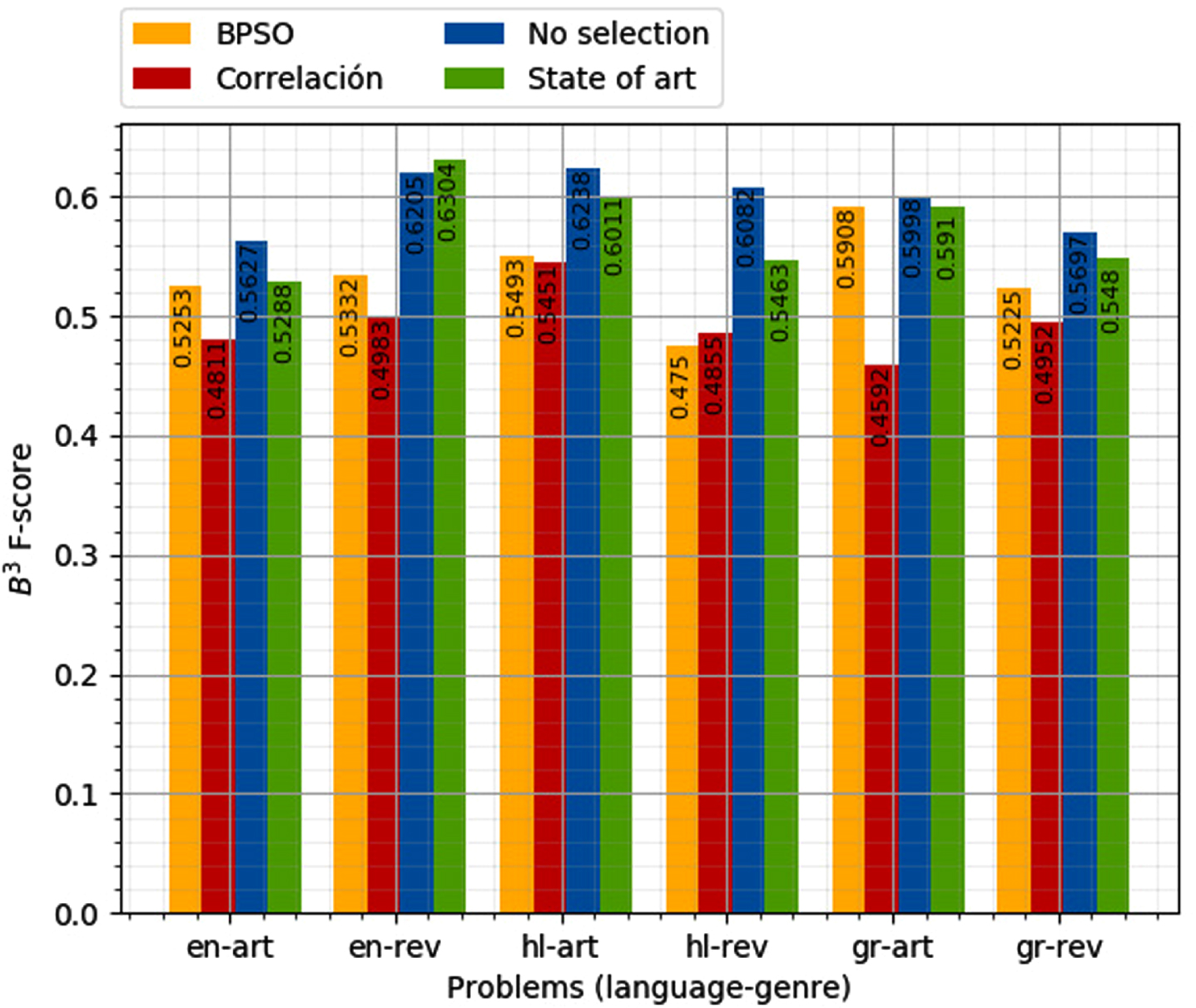
Comparison of the B³ F-score of feature selection with BPSO, correlation and no selection and state of the art (training dataset PAN 2017).

Fig. 2

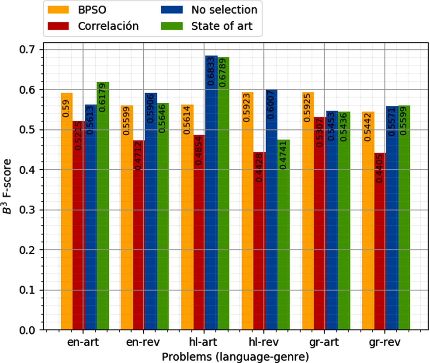
Comparison of the B³ F-score of feature selection with BPSO, correlation and no selection and state of the art (test dataset PAN 2017)

4.4 Weighted cosine similarity

Using the proposed feature extraction, log-entropy weighting, and feature selection using MAD (the method with the best performance), a hierarchical agglomerative clustering algorithm was used to determine the clusters (average). This algorithm was applied with the normal cosine distance and with the weighted cosine distance. The index Caliński-Harabaz was used to determine the number of clusters.

The w (from Eq. 5) value was determined with the training dataset. Table 10 shows the best result for the training. In 5 out of 6 categories (language-genre), weighted cosine had the best result.

Table 10
Results of using the weighted cosine similarity x_w and y_w equal. The value of w per category is the one with the best performance for the training dataset. MWC is the Modified Weighted Cosine; OCD is the Original Cosine Distance

Language, genre B³ F-score

w MWC OCD

English-articles 0 0.5716 0.5627

English-reviews 1 0.6205 0.6205

Dutch-articles 0.1 0.6314 0.6238

Dutch-reviews 0.2 0.6093 0.6082

Greek-articles 0.2 0.6108 0.5998

Greek-reviews 0.2 0.5742 0.5697

Average 0.6030 0.5974

Language, genre	B³ F-score
English-articles	0	0.5716	0.5627
English-reviews	1	0.6205	0.6205
Dutch-articles	0.1	0.6314	0.6238
Dutch-reviews	0.2	0.6093	0.6082
Greek-articles	0.2	0.6108	0.5998
Greek-reviews	0.2	0.5742	0.5697
Average		0.6030	0.5974

The highest B³ F-score value resulting from the variations from 0 to 1 of w in the training dataset was the one used for each problem (considering language and genre) in the test dataset. Table 11 shows the result and a comparison with results with the original cosine distance and the state of the art. Using weighted cosine distance improves the results in three out of six of the categories regarding the cosine distance; the most representative improvement is in English-articles however, this improvement was not enough to get the best result compared with the state of the art. Contrarily, there was an important decrease in the value obtained in Dutch-articles.

The average shows an improvement in the use of the weighted cosine distance and generally more stable results (around 60 percent for the majority of the categories).

Table 11

Results of using the weighted cosine similarity x_w and y_w equal in the test dataset. The value of w per category was kept for the value of the training. MWC is the Modified Weighted Cosine; OCD is the Original Cosine Distance

Language-genre	B³ F-score
	w	MWC	OCD	State of the Art
English-articles	0	0.5867	0.5613	0.6179
English-reviews	1	0.5906	0.5906	0.5646
Dutch-articles	0.1	0.6620	0.6833	0.6789
Dutch-reviews	0.2	0.5986	0.6007	0.4741
Greek-articles	0.2	0.5455	0.5453	0.5436
Greek-reviews	0.2	0.5630	0.5571	0.5599
Average		0.5911	0.5897	0.5732

4.5 Comparison per-category with the state of the art

In this section, a comparison with the best results of the state of the art (per category) was made. Table 12 shows the results. The proposal in this article improves the results in two categories (English-articles and Greek-reviews), while the proposal of the other three authors had the best result in the other four categories. On average, the joint results of the state of the art had the best result; despite this, following the same approach for the full dataset, the proposal in this article had the best result.

Table 12
Comparison of the proposal with the best result per category of the state of the art. BoSotApC is the Best of State of the Art per Category

Language-genre B³ F-score

Proposal BoSotApC - Author

English-articles 0.587 0.618 - [7]

English-reviews 0.591 0.578 - [6]

Dutch-articles 0.662 0.679 - [7]

Dutch-reviews 0.599 0.603 - [6]

Greek-articles 0.545 0.566 - [8]

Greek-reviews 0.563 0.552 - [7]

Average 0.5988 0.5993

Language-genre	B³ F-score
English-articles	0.587	0.618 - [7]
English-reviews	0.591	0.578 - [6]
Dutch-articles	0.662	0.679 - [7]
Dutch-reviews	0.599	0.603 - [6]
Greek-articles	0.545	0.566 - [8]
Greek-reviews	0.563	0.552 - [7]
Average	0.5988	0.5993

5 Discussion

The use of special punctuation allows identifying more aspects related to the style of the authors. Identifying each category of n-grams (adding a suffix) facilitates the identification of the different linguistic aspects.

The size of the texts (with a length between 100 and 500 characters) was not favorable to improve the maximum value obtained (0.6030 for the training dataset and 0.5911 for the test dataset); however, it was possible to overcome the best approach of the PAN 2017 (0.5743 for the training dataset and 0.5732 for the test dataset).

Feature selection using the correlation algorithm was the one with the worst performance. This could be due to the number of features selected tending to be smaller than the used for authorship attribution (around 500 dimensions).

Features selection using BPSO had a better average performance for some categories (language-genre) compared with the other methods of features selection, despite this, the algorithm has some problems to converge.

Filters for feature selection had the best performance. Both filters have a better B³ F-score than the state of the art. The filter based on MAD had the best performance, this could be related to the absence of the square in the equation; the MAD value gives a better approximation of the values regarding the average, so the scattered data is ignored.

The idea behind the weighted cosine distance is to give more importance to those dimensions where the vectors (representing the documents) are similar. Using this measure when clustering, can be considered as an extra filter for features.

6 Conclusion

In this work, through the use of specific features extractions, the use of filter MAD for feature selection and the use of weighted cosine distance as input for the hierarchical agglomerative clustering resulted in an improvement over the state of the art.

The method proposed for features extraction, unlike the one used by [7], captures a better separation of words per language; an improvement of +0.0127 in the test dataset, using this method, was achieved.

The correlation algorithm could have a better performance if a minimum number of features is set and the threshold redundant is increased.

Similarly, feature selection based on BPSO with a non-binary representation of the features could be used to improve the results.

The weighted cosine distance with different values of w for each vector could represent a performance improvement; investigation related to this topic to determine the values to set the values of w is required. However, the use of the same value of w gives an improvement regarding the cosine distance for some categories.

As future work, the use of embeddings for features representation and deep learning algorithms for clustering is propose.

Footnotes

Acknowledgment

The work was done with support from the Mexican Government through the grant A1-S-47854 of the CONACYT, Mexico and grants 20211784, 20211884, and 20211178 of the Secretaría de Investigación y Posgrado of the Instituto Politécnico Nacional, Mexico. The authors utilized the computing resources brought to them by the CONACYT through the Plataforma de Aprendizaje Profundo para Tecnologías del Lenguaje of the Laboratorio de Supercómputo of the INAOE, Mexico.

References

Abualigah

L.M.

, Khader

A.T.

and Hanandeh

E.S.

, A new featureselectionmethod to improve the document clustering using particleswarm optimization algorithm, Journal of Computational Science25 (2018), 456–466.

Amigó

, Gonzalo

, Artiles

and Verdejo

, A comparison ofextrinsic clustering evaluation metrics based on formal constraints, Information retrieval12 (2009), 461–486.

Batyrshin

, Kubysheva

, Solovyev

and Villa-VargasVisualization

, of similarity measures for binary data and2×2 tables, Computación y Sistemas20(2016), 345–353.

Dara

and Reddy

T.R.

, Authorship attribution using content basedfeatures and n-gram features, International Journal ofEngineering and Advanced Technology9 (2019), 1152–1156.

Ferreira

A.J.

and Figueiredo

M.A.

, Efficient feature selectionfilters for high-dimensional data, Pattern Recognition Letters33 (2012), 1794–1804.

García-Mondeja

, Castro-Castro

, Lavielle-Castro

and Munoz

, Discovering Author Groups Using a β- compact Graph-based Clustering, In CLEF 2017 Working Notes CEUR Workshop Proceedings, 2017.

Gómez-Adorno

, Aleman

, Vilariño

, Sanchez-Perez

M.A.

, Pinto

and Sidorov

, Author Clustering using Hierarchical Clustering Analysis, In CLEF 2017 Working Notes CEUR Workshop Proceedings, 2017.

Halvani

and Graner

, Author Clustering based on Compression-based Dissimilarity Scores, In CLEF 2017 Working Notes CEUR Workshop Proceedings, 2017.

Kocher

and Savoy

, UniNE at CLEF 2017: Author Clustering, In CLEF 2017 Working Notes CEUR Workshop Proceedings, 2017.

10.

Liu

, Kang

, Yu

and Wang

, A comparative study on unsupervised feature selection methods for text clustering, In 2005 International Conference on Natural Language Processing and Knowledge Engineering, 2005, pp. 597–601.

11.

Mahor

and Das

, Performance evaluation of various featureextraction and classification techniques for authorship attribution, International Journal of Innovation and Scientific Research16 (2015), 252–259.

12.

Markov

, Stamatatos

and Sidorov

, Improving Cross-Topic Authorship Attribution: The Role of Pre-Processing, In Proceedings of the 18th International Conference on Computational Linguistics and Intelligent TextProcessing CICLing 2017. Springer, 2017.

13.

Martín-del-Campo-Rodríguez

, Sidorov

and Batyrshin

I.Z.

, Enhancement of Performance of Document Clustering in the Authorship Identification Problem with a Weighted Cosine Similarity, In I.Z. Batyrshin, M. de Lourdes Martínez-Villaseñor, and H.E.P. Espinosa (Eds.), Advances in Computational Intelligence – 17th Mexican-InternationalConferenceonArtificial Intelligence, MICAI 2018, Guadalajara, Mexico, October 22–27, 2018, pp. 49–56.

14.

Pedregosa

, Varoquaux

, Gramfort

, Michel

, Thirion

, Grisel

, Blondel

, Prettenhofer

, Weiss

, Dubourg

, Vanderplas

, Passos

, Cournapeau

, Brucher

, Perrot

and Duchesnay

, Scikit-learn: Machine Learning in Python, Journal ofMachine Learning Research12 (2011), 2825–2830.

15.

Pramokchon

and Piamsa-nga

, An unsupervised, fast correlation-based filter for feature selection for data clustering, In Proceedings of the First International Conference on Advanced Data and Information Engineering, Springer Singapore, 2013, pp. 87–94.

16.

Sapkota

, Bethard

, Montes-y-Gómez

and Solorio

, Not All Character N-grams Are Created Equal: A Study in Authorship Attribution, In Proceedings of the 2015 Annual Conference of the North American Chapter of the ACL: Human Language Technologies. NAACL-HLT-15. Association for Computational Linguistics, 2015, pp. 93–102.

17.

Sidorov

, Syntactic n-grams in computational linguistics. (1st ed.). Springer International Publishing, 2019.

18.

Stamatatos

, A survey of modern authorship attribution methods, Journal of the American Society for Information Science andTechnology60 (2009), 538–556.

19.

Tschuggnall

, Stamatatos

, Verhoeven

, Daelemans

, Specht

, Stein

and Potthast

, Overview of the Author Identification Task at PAN-2017: Style Breach Detection and Author Clustering, In Working Notes of CLEF 2017 – Conference and Labs of the Evaluation Forum, Dublin, Ireland, September 11–14, 2017.

20.

and Wunsch

, Survey of clustering algorithms, IEEETransactions on Neural Networks16 (2005), 645–678.

Unsupervised authorship attribution using feature selection and weighted cosine similarity

Abstract

Keywords

1 Introduction

2 Related work

2.1 Proposed models for the edition of PAN 2017

3.1 Description of the dataset

3.3 Word n-grams

3.3.1 N equal to 1

3.3.2 N different to 1

3.4 Character n-grams

3.5 Typed character n-grams

3.5.1 Affix n-grams

3.5.2 Word n-grams

3.5.3 Punctuation n-grams

3.6 Feature selection

3.6.1 Feature selection based on filter

3.6.2 Feature selection using binary particle swarm optimization

Table 3 Solution representation for the feature selection using BPSO X 0 1 1 -1 -1 1 0 -1 1 0

4.1 Evaluation

4.2 Pre-processing and feature extraction

4.3.1 Feature selection based on filters

6 Conclusion

Footnotes

Acknowledgment

References

Table 3
Solution representation for the feature selection using BPSO

X 0 1 1 -1 -1 1 0 -1 1 0