The new approaches for solving hierarchical Chinese postman problem with stochastic travel times

Abstract

The hierarchical Chinese postman problem (HCPP) aims to find the shortest tour or tours by passing through the arcs classified according to precedence relationship. HCPP, which has a wide application area in real-life problems such as shovel snow and routing patrol vehicles where precedence relations are important, belongs to the NP-hard problem class. In real-life problems, travel time between the two locations in city traffic varies due to reasons such as traffic jam, weather conditions, etc. Therefore, travel times are uncertain. In this study, HCPP was handled with the chance-constrained stochastic programming approach, and a new type of problem, the hierarchical Chinese postman problem with stochastic travel times, was introduced. Due to the NP-hard nature of the problem, the developed mathematical model with stochastic parameter values cannot find proper solutions in large-size problems within the appropriate time interval. Therefore, two new solution approaches, a heuristic method based on the Greedy Search algorithm and a meta-heuristic method based on ant colony optimization were proposed in this study. These new algorithms were tested on modified benchmark instances and randomly generated problem instances with 817 edges. The performance of algorithms was compared in terms of solution quality and computational time.

Keywords

Optimization arc routing problems chance-constrained stochastic programming new efficient algorithm hierarchical Chinese postman problem

1 Introduction

The goal of the arc routing problems is to establish the shortest tour or tours that return to the starting point by stopping at least once at all arcs on a network [1]. In this study, Hierarchical CPP (HCPP), which considers the precedence relationship between the arcs was discussed. The most typical real-life examples of HCPP are activities such as garbage collection, street cleaning, snow shoveling, road maintenance, and repair which consider the precedence relationships between roads. HCPP attempts to find the optimal tours that traverse each arc in the offered network at least once, taking into account precedence relations of the paths roads (arc) in a given network.

A stochastic Vehicle Routing Problem (SVRP) occurs when one or more deterministic Vehicle Routing Problem (VRP) parameters are random. Because of the uncertainty, it includes SVRP that is more similar to real-life problems. Customers, inquiries, travel times, or service times may be random elements of this sort of issue. In the present era where the competitive environment is at its peak, it is necessary to know the travel times between nodes in order not to lose time for corporations in the public and private sectors and to avoid a reduction in the quality of the services while enabling accurate planning. It is an undeniable fact that optimal route planning needs to be generated by taking factors such as distance and time into consideration which are deemed essential for companies and customer satisfaction procedures. Yet, owing to unpredictable weather conditions, environmental circumstances, or traffic, it is not often feasible to articulate travel times and speeds with exact values. On the very same day, although the travel times rely on the distance, it may be stochastic due to accidents or multiple factors that hinder transport. In the literature, this form of problem, which was first discussed by Kao in 1978 expresses the stochastic state of traffic, is referred to as vehicle routing problem with Stochastic Travel Times (STT-VRP) or vehicle routing problem with Stochastic Service Times (SST-VRP) [2].

Concerning the literature research, most HCPP-related studies have used the distances while the arrival times, which differ due to uncertainties have not been taken into consideration. However, in urban traffic we experience in real life, the travel time between nodes is not constant owing to changing traffic intensity and weather conditions. Because of this uncertainty, HCPP has been solved within the scope of this study by using the chance-constrained stochastic programming method. Thus, it was shown that the STT-HCPP which was addressed within the scope of this paper, is a different form of problem that has never before been observed. In particular, a mathematical model for HCPP has been established in prior studies, and it can be stated that the mathematical model formed due to the problem’s NP-hard nature offers suitable solutions only for small-sized problems. Two new algorithms, one heuristic, and the other meta-heuristic were suggested within the framework of this study, to determine the best answer to the problem in a reasonable time. Sensitivity analyses on meta-heuristic were also performed concerning the different number of ants and number of iterations. It is also critical that the proposed new methods are focused on the chance-constrained stochastic approach. It is aimed at the problem type and suggested solution approaches to adapt HCPP to real life and to be the first study in the literature.

Briefly, the two main scientific contributions of this paper were described below.

This research is the first study to solve HCPP using a chance-constrained stochastic programming approach while taking into account the stochasticity of travel times in HCPP and as well as assuming that these parameters are appropriate for a certain distribution. In several of the VRP and Traveling Salesman Problem (TSP) studies [3, 4], which are the most general implementation areas of node routing problems before [3, 4] travel times and/or costs are regarded as stochastic. However, there is no similar study for HCPP which is an edge routing problem. A new STT-HCPP problem form was therefore introduced in this study.

In this study, two new algorithms were proposed for the solution of large-size STT-HCPP problems, which are easier to apply to real-life problems owing to the uncertainty it includes. The first is the heuristic method based on the Greedy Search (GS) algorithm, while the second is a meta-heuristic method based on ant colony optimization (ACO). The purpose of these methods is to find solutions to large-size problems in a brief time. Algorithms were tested and compared for their effectiveness by using these methods for test problems.

1.1 Literature survey

In this section, firstly, studies related to HCPP in the literature were discussed, and then studies related to stochastic parameters of CPP, STT-SVRP, and STT-TSP were examined, respectively.

HCPP was first proposed by Dror et al. by addressing a network of arcs divided into classes in which precedence relationships were described [5]. They demonstrated that the issue can be resolved in polynomial time if the precedence relationships are linear, and all sub-graphs are entangled in the hierarchy classes. In general, they proved that the problem is in the NP-hard class. In [6], the authors addressed a more rational scenario in which subgraphs are not entangled in hierarchical classes. In their study, they proposed an approach to the heuristic solution for HCPP that can be especially used in snow shoveling. In [7], the author developed a new heuristic method for the combination of disconnected hierarchical classes. It was claimed that this method established in the study accomplished better results than the heuristic model of Alfa and Liu [6]. In [8], the authors suggested an algorithm that needs less computational work and offers a clear solution in a shorter period than earlier studies. In this study, the first algorithm which provides a precise solution for HCPP was discussed. In [9], the authors established a method for converting the HCPP into an equivalent Rural Postman Problem. They suggested a splitting heuristic for unidirectional HCPP with linear precedence relations. The converted problem was subjected to a branch and cut algorithm to overcome HCPP, which has two objectives, namely, the hierarchical purpose and production time. In [10], the authors developed an existing algorithm that solves HCPP in their work and they reduced the time complexity of the original algorithm with their optimistic technique to the O(kn⁴) (where k is the number of layers in the graph and n is the number of nodes). Under such an algorithm, each sub-network’s distinct minimum cost routes were determined according to precedence levels. In [7], the authors established a heuristic approach that offers improved lower HCPP bound values compared to CPP. With this lower bound value, it was decided that in algorithms that provide exact solutions such as branch and bound algorithms, the optimum solution was achieved in a shorter period. In [11], the authors suggested a recent algorithm focused on the methodology of cell separation for efficient coverage of a defined location packed with random obstacles. First, the cells were separated into pieces in this hierarchical method, then, the CPP was resolved to determine a Euler tour that travels through these cells. In [12], the authors proposed a new method to eliminate the time complexity of algorithm O (kn⁵) (by Dror in [5]) and used the Kruskal method to reduce the number of edges in a network that has a time complexity of O (k²n²). In [13], the authors discussed the hierarchical mixed RPP in their study. A branch and cut algorithm offering a certain solution to the problem was presented in the study, and it has been shown that the results achieved with the algorithm were more effective and efficient than other existing methods. In [14], the authors discussed time-dependent HCPP when travel time changes according to the time of the day. A mixed-integer mathematical model for problem-solving was established in the research, and the genetic algorithm (GA) and hybrid simulated annealing were suggested as a solution approach to large-scale problems.

To the best of our knowledge, there are no studies in the literature concerned with stochastic travel times concerning HCPP. On the other hand, there is a very limited number of studies on the stochastic parameters of CPP. In [15], the authors addressed the CPP in the studies of networks with stochastic travel times. They proposed an algorithm as a solution. In [16], the authors studied three uncertain programming models for CPP with uncertain weights. They claimed that these models could be transformed into deterministic equivalent models. They used Dijkstra’s algorithm and Fleury’s algorithm to solve the problem. In [17], the authors proposed multi-objective CPP under the framework of uncertainty theory for an undirected connected network. They presented an expected value model as a solution approach.

There has been no prior research on STT-HCPP, as far as we know. However, a review of the related literature indicates that research on STT-SVRP and STT-TSP is present. Studies in this field were reached by entering the word group “stochastic routing problems” into the Web of Science (WoS) database. Keyword network analysis was performed using the VOSviewer (Version 1.6.9) package program. According to the bibliometric analysis made using the VOSviewer program, the most used keywords are those shown in Fig. 1.

Fig. 1

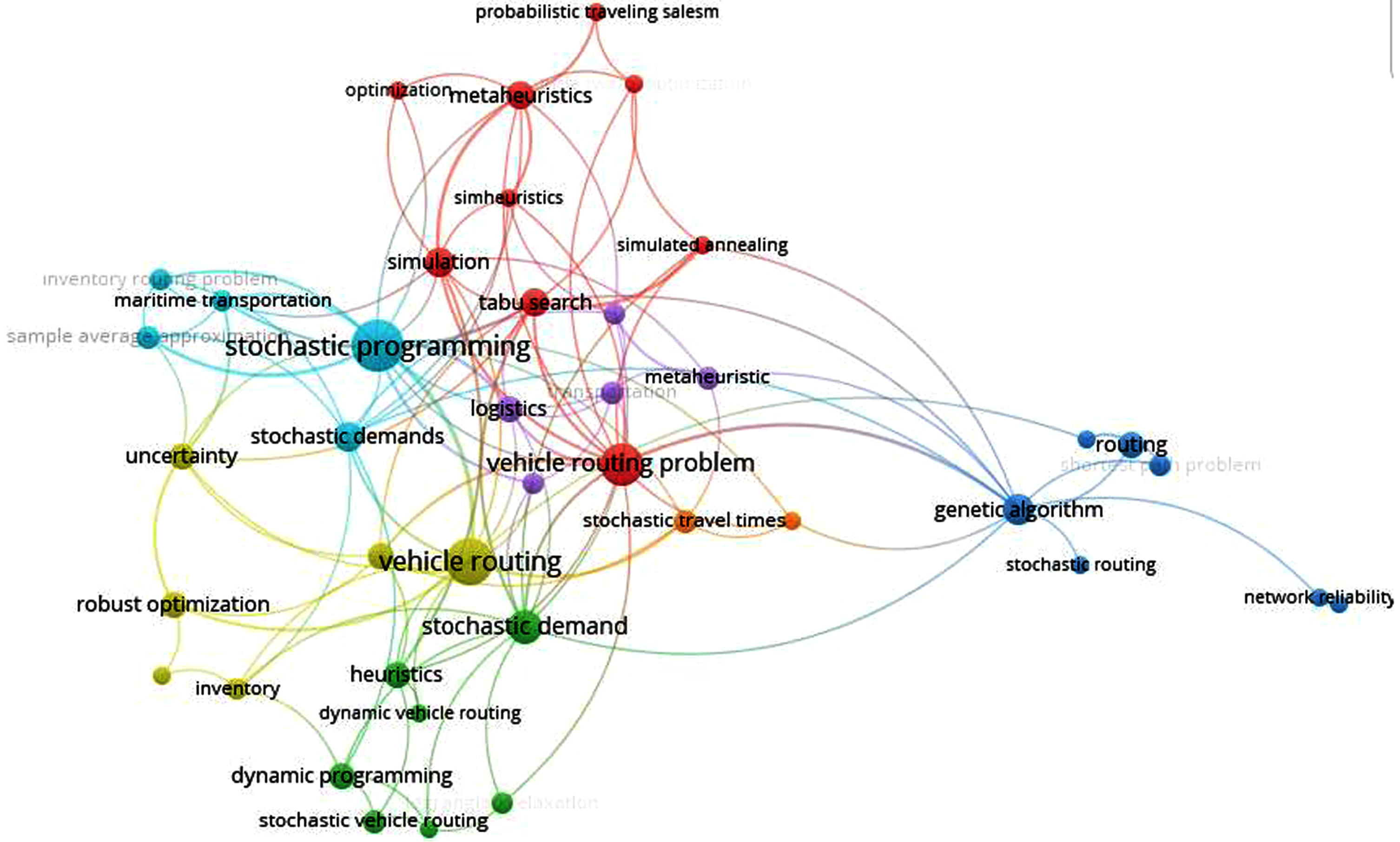
Keyword network analysis (VOSviewer).

As can be seen from Fig. 1, among the most used keywords in stochastic routing problems are “stochastic programming”, “vehicle routing”, and “stochastic demand”. In addition, it is seen that metaheuristic algorithms such as GA and simulated annealing used for the solution of large-scale problems are among these keywords. Some of the studies related to fuzzy routing problems were given in this section. In [2], the author discussed the TSP with stochastic travel time (STT-TSP) for the first time. In this research, a dynamic programming-dependent heuristic algorithm was suggested for problem-solving. In [18], the authors established generalized dynamic programming for STT-TSP, which even in the absence of uniformity, guarantees an optimum level. In [19], the authors conducted a study on stochastic travel and service time-based VRP. A banking example was examined in this study. For the issue under discussion, they proposed three separate models including the chance-constrained model. For the solution of these models, they proposed the branch and cut algorithm. In [20], the authors focused on SVRP on a network with random travel and service times in the study. Two stochastic programming models have been developed in the study. The first model minimizes the estimated delivery period, while the second model maximizes the likelihood of project completion at a specified period. In [21], the authors addressed the topic of vehicle routing in a stochastic network, utilizing real-time traffic information. A decision-making process was built in this research, based on the Markov decision procedure (MDP). In [22], the authors worked with the planning of truck routes within stochastic networks. A methodology for forecasting the arrival times of the customers was suggested in the process described in this study since travel and service times are uncertain. An approximate solution based on dynamic programming was provided using the estimated time of arrival. In [23], the authors studied vehicle routing with soft time windows and erlang travel times. In this research, travel times fit the gamma distribution. A tabu search algorithm was developed to solve the problem. In [24], the authors studied a TSP traveling with time windows and stochastic and dynamic travel time. In the research, it was presumed that arrival times in nodes were normally distributed, and a heuristic method for solving the problem was established. In [25], the authors addressed VRP with uncertain demand and travel time parameters to mitigate unmet demand. In the study, a chance-constrained programming technique was used, and a tabu search heuristic method was proposed to solve the model. In [26], the authors suggested a stochastic programming model that would take stochastic demand and travel time into account and introduced a GA created to solve this problem In [27], the authors examined a VRP with time windows and stochastic travel and service times in their study. The problem was modeled according to two different approaches namely the chance-constrained model and the two-stage stochastic programming with recourse model. A heuristic method based on tabu search which takes into account the stochastic nature of the problem was presented to overcome both models effectively. In [28], the authors have studied VRP with hard time windows and stochastic service times. In the study, it was accepted that the service times fit symmetrical triangular distribution and the chance-constrained stochastic programming model was used. In [3], the authors analyzed the VRP with stochastic travel times including soft time windows and service costs. The gamma distribution was used for travel time in the study. For the model’s solution, a tabu search method was suggested. In [29], the authors addressed the issue of stochastic vehicle orientation with soft time windows under uncertain travel and service time. They introduced a new stochastic programming model to reduce the carrier’s total expense, thus guaranteeing the likelihood of arrival to every customer in the minimum time. A recursive tabu search heuristic was developed to solve the problem. In [30], the authors examined VRP with hard time windows and stochastic service times. They used chance-constrained programming to model the problem. The study results indicated that the approach proposed is effective and that a stochastic chance-constrained model has benefits over deterministic models. In [31], the authors suggested a memetic algorithm for solving a VRP with time windows and stochastic travel and service times. The effects of the proposed Multipurpose Memetic Algorithm and the Multi-objective Recursive Local Search algorithms were contrasted, and their efficacy was demonstrated. In [32], the authors studied the problem of vehicle routing with a time window and stochastic travel times. A method for estimating the distribution of the initial service times and arrival times was suggested in the research. The results of the research demonstrate how solutions are influenced by adjusting customer care standards, distribution of travel time, and different parameter settings. In [33], the authors discussed VRPs with stochastic service and travel times. In the study, the mentioned time was examined concerning the triangular distribution. The model was first approached using a branch and cut algorithm or a Lagrange parsing method, and then, a heuristic method was used to create the solution. In [34], the authors studied the problem of VRP with hard time windows and stochastic travel and service time in their study. Travel and service times were regarded as parameters with normal distribution in this research, but it was noted that arrival times with normal distribution were not well modeled. A meta-heuristic based on Recursive Local Search was proposed for the solution to the problem. In [35], the authors focused on solving the stochastic VRP with time windows under uncertainty. In the research, given the complicated nature of chance-constrained stochastic programming, some measures were recommended for the uncertainties in the specific problem. Suggested suitable steps to solve the problem were introduced into an existing heuristic method of tabu-search. In [36], the authors studied the problem of multi-objective VRP with hard time windows and stochastic travel time and service time. Travel and service times were modeled as normal distribution in the study. Two separate algorithms were suggested for the solution to the problem, namely the Memetic Algorithm and Recursive Local Search, and the results were compared. In [37], the authors introduced some constrained covering solid TSPs in their study. In real-life situations, since some parameters cannot be expressed with crisp values, traveling costs are regarded as rough variables in their study. Covering distance is considered both a fuzzy and a rough variable. A new heuristic algorithm was suggested as a solution approach. In [38], the authors discussed the uncertain multi-objective multi-item fixed charge solid transportation problem with budget constraints. In the model suggested, many variables such as transportation costs, and transportation times were assumed as uncertain variables. In the uncertain model, the parameters were treated as zigzag and normal uncertain variables. Under the uncertainty theory, three different models, namely the expected value model, the chance-constrained model, and the dependent chance-constrained model were developed. Equivalent deterministic transformations of these models were generated, and they were solved through three different methods, which are the fuzzy programming method, linear weighted method, and global criterion method. In [39], the authors presented a new approach to the solution of open VRP. In this new method, the GA and modified Kruskal’s method were hybridized. This suggested approach is adaptable to real-life cases, and the obtained results of the suggested method have been compared with evolutionary methods. In [40], the authors examined the route-based MDP framework for stochastic dynamic routing problems. In this study, modeling techniques and solution methods used in the literature were compared. In [41], the authors have studied VRP with a makespan objective incorporating both stochastic and correlated travel times. A new method for solving the problem has been developed and the effect of the different correlation levels on the value of the objective function has been demonstrated. In [42], the authors examined the capacitated VRP under an uncertain paradigm. A fuzzy model was constructed for uncertain travel time and cost. As a solution approach, a hybrid metaheuristic algorithm based on GA and bacteria foraging optimization algorithm was designed. In [43], the authors discussed the Time Capacitated Arc Routing Problem with stochastic demands. To solve the problem, a strategic oscillation simheuristic algorithm was proposed. In [44], the authors presented a stochastic service network design model with an integrated VRP. A sample average approximation approach was proposed to solve the problem and combined with an iterated local search heuristic. In the study, a case study based on data for transport orders of a German freight forwarding company was discussed. In [45], the authors discussed a time-dependent VRP with soft time windows and stochastic factors. A Hybrid Algorithm was developed to solve the model. The sweep Algorithm and Improved Particle Swarm Optimization were combined. In [46], the authors addressed the issue of flying sidekick TSP with stochastic travel time. The problem was formulated as an MDP. The deep Q-network and Advantage Actor-Critic algorithms were proposed for the solution of MDP formulation.

When reviewing the HCPP studies in the literature, it was found that several of these studies do not take into consideration the travel times between nodes but acknowledge the distances between nodes. In addition, there was no research on this topic that deals stochastically with travel times. In order to fill this gap in the literature with this study, HCPP with Stochastic Travel Times (STT-HCPP), which is a new problem form, was taken into account. It was agreed in the analysis that travel times, which represent randomness, were normally distributed.

2 Preliminaries

2.1 Stochastic programming

Difficulties were generally experienced while trying to determine the values of model parameters (c_j,a_i,j, b_i) used in modeling real-life problems with linear programming. In this context, taking the parameter values as exact values by utilizing existing evidence or past studies is not a correct approach since it may impact the study’s impartiality. Moreover, model parameters do not necessarily have exact values but are represented with random variables. Problems that contain some or all of the parameters of their model as random variables are named stochastic programming problems (SPP) [47]. Concerning the Stochastic programming that George Dantzig first proposed in the 1950 s, substantial improvement has been achieved in understanding model properties and developing algorithmic methods to solve them [48].

Stochastic programming is one of the most commonly employed techniques for routing problems, where parameter values are hard to express as exact values. And also, the amount of garbage to be collected before the vehicle reaches the specific places cannot be identified precisely in real-life issues, in a garbage collection process. Likewise, even though the vehicle is always traveling on the same road path, the duration of the travel cannot be described with exact values, since the arrival times can vary due to weather and environment. Again, the punctuality of a flight can vary depending on weather conditions.

SVRP occurs when some parameters of Classic VRP are random. The most common examples of this are stochastic travel time and stochastic demands [49].

Among the SVRP studies which were analyzed, some have explored creating a suitable mathematical model and approaches to solutions. In some studies, it was aimed to suggest algorithms for the solution of SVRP. Looking once again at the literature studies when building the mathematical model, it is shown that SVRP’s chance-constrained stochastic programming and stochastic programming with recourse approaches were used [50]. For example, in [51] the authors suggested some reduction methods for type-2 fuzzy variables in a transportation problem, and the proposed models were reduced to chance-constrained programming problems with different credibility labels.

2.1.1 Chance-constrained stochastic programming

First introduced by Charnes and Cooper in [52] chance-constrained stochastic programming is about revealing the parameters that are random variables of a certain distribution of probability and expressing this probabilistic framework with the function of probability in the objective function and the constraints of the problem. The chance-constrained linear programming model is defined as follows; $\max (\min) Z^{(k)} (x) = \sum_{j = 1}^{n} c_{j}^{(k)} . x_{j} k = 1, . ., K$ (1)

$\begin{matrix} P [\sum_{j = 1}^{n} a_{ij} . x_{j} ⩽ b_{i}] ⩾ 1 - \propto_{i}, \\ i = 1, 2, 3, \dots . ., m \end{matrix}$ (2) $x_{j} ⩾ 0, j = 1, 2, \dots, n$ (3) $\propto_{i} (0, 1) i = 1, 2, \dots . ., m$ (4)

In the model, the c^(k), a_i,j, and b_i are model parameters, and some or all of them are random variables. ∝iare the predetermined possibilities. Here decision variables of x_j have a deterministic structure [53]. The stochastic parameters in the model must have certain distribution and probability levels ∝i should be determined. The model is solved using this information by rendering it a deterministic form [54].

2.1.1.1. Chance-Constrained Models whose Coefficients are Random Variables with Normal Distribution. In linear programming problems where at least one of the coefficients of $c_{j}^{(k)}$ , a_i,j and b_i is a random variable, it is assumed that these coefficients generally show normal distribution characteristics. Under this assumption, in the chance-constrained stochastic linear programming problem modeled in Section 2.1 $c_{j}^{(k)}$ , a_i,j and b_i are random variables with a normal distribution [55].

The only parameter that can be considered stochastic in HCPP is the objective function coefficients, $c_{j}^{(k)}$ , within the scope of this study the case in which “only $c_{j}^{(k)}$ coefficients are random variables” will be discussed.

Let’s assume $c_{j}^{(k)}$ , are random variables with a normal distribution and the z^(k) is the k^th objective function. The mean of E (z^(k)) is given in the form of E (z^(k)) Here the deterministic linear programming equation referring to the problem of probabilistic linear programming is as follows: $E (z^{(k)}) = \sum_{j = 1}^{n} E (c_{j}^{(k)}) x_{j}, k = 1, . ., K$ (5)

Here, $E (c_{j}^{(k)})$ is the mean of $c_{j}^{(k)}$ . Thus, the deterministic objective function that has the expected value model (E-model) will be as follows [47]. $\max (\min) = E (z^{(k)}) = \sum_{j = 1}^{n} E (c_{j}^{(k)}) x_{j}, k = 1, . ., K$ (6)

2.2 Mathematical formulation

For the HCPP belonging to the NP-hard problem class, paths/arcs are divided into classes and a precedence relationship is defined in these classes [5]. Therefore, in HCPP the order in which the paths/arcs are to be followed is set beforehand. The object of this type of problem is to establish the shortest tour/tours considering the precedence relationships and by traveling through each arc/path at least one time in a hierarchical network. Snow removal and salt dumping activities, where roads are categorized according to their importance (urban or rural, main road, secondary road, etc.) are one of the best examples that can be offered for HCPP in real life. Concerning these procedures, when the aforementioned procedures are performed on the main roads of the first precedence class firstly, and all the main roads are completed, we may pass to other roads.

One of the most important assumptions belonging to linear programming is the fact that model parameters have a deterministic structure. The classical mathematical model of HCPP is very useful in this context. However, these parameters take place in an uncertain way in most real-life problems. This uncertainty resulting from different factors can’t be represented with mathematical models. Therefore, chance-constrained stochastic programming has been used in this study to include this uncertainty in mathematical models. Most of the data excepted as exhibiting normal distribution since it would be more suitable for real life in terms of statistics. Therefore, within the scope of this study, c_ij objective function coefficients that show the travel time between two nodes in HCPP were considered random variables with normal distribution characteristics, and the model was transformed into STT-HCPP by making use of “the case where the only coefficients of c_j are random variables” which are explained in Section 2.1.1.1.

Let’s consider a G (V,E) network where V represents the set of nodes and E is a non-directional set of arcs (paths). This network is divided into m different sub-networks, each of these representing a hierarchical level. In this case, a hierarchical network is shown as; G (V,E) = G₁(V₁,E₁) ∪ G₂(V₂,E₂) ∪. . . ∪ G_m(V_m,E_m) [56]. Here, G_m is the mth sub-network showing the arcs/ roads that will be traveled on the mth order.

The indexes, sets, parameters, and decision variables used in the HCPP integer linear programming model are shown below under respective titles [14].

Indexes;

i,j: Nodes on the network

t: Number of the edge traversal in the route (steps)

h: Hierarchical levels.

Sets;

i, j / V: Set of vertices i, j = {1, 2, . . . , n},

h / H: Set of hierarchies {1, 2, . . . , h},

t≤L: Number of steps L = 2 ∥E∥

E _h : Set of edges of h^th hierarchy class

E: Set of all edges in the network, E = {E ₁ ∪ E ₂ ∪...∪ E _h }

∥E∥: The total number of edges of h^th hierarchy class

δ_h(i): The edges of E_h set that exist from node i, δ_h (i) ={ j^|(i,j) ∈ E_h }.

δ(i): Set of all edges that exist from node i, δ (i) =⋃ _hɛH δ_h (i) = { δ₁ (i) ∪ δ₂ (i) ∪ … ∪ δ_h (i) }

Parameters;

C _ij : Distance matrix of the edge (i, j)

B _ij : Connection matrix of the edge (i, j)

O _ij : Precedence matrix of the edge (i, j)

M: Is a sufficiently large number

n: The total number of nodes in the graph.

Variables;

$x_{ij}^{t} = {\begin{matrix} 1 \\ 0 \end{matrix}$ if traversed from node i to node j at t^th step1, otherwise 0.

$y_{ij}^{t} = {\begin{matrix} 1 \\ 0 \end{matrix}$ if traversed from node i to node j at t^th step for the first time 1, otherwise 0.

$φ_{ht} = {\begin{matrix} 1 \\ 0 \end{matrix}$ if traversed from all edges of h^th hierarchy in t^th step completed 1, otherwise 0.

Using this information, HCPP’s mixed-integer linear programming model can be written as follows [14]. This model is deterministic. The general aim of the paper is to handle the problem stochastically in order to make this deterministic model found in the literature more suitable for a real-life problem. In the mathematical model formulation, the arrival time between the nodes was taken as the basis instead of the distance in the objective function and it was aimed to minimize these times. Because, it is not always possible to express travel times with crisp values due to uncertain weather conditions, environmental conditions, or traffic conditions. Even on the same day, travel times between centers may vary due to different reasons such as accidents or construction-repair works that will prevent transportation. Stochastic programming is used to express these uncertainties arising from various reasons in the HCPP mathematical model. In this model; when the objective function coefficients of c_ij are considered as random variables with normal distribution characteristics, the problem transforms into STT-HCPP. As a matter of fact, the only parameter that can be considered stochastic due to the nature of HCPP is the objective function coefficients c_ij, which represent the travel times between nodes. Therefore, when the objective function coefficients are considered as random variables with c_ij normal distribution, the objective function z will also display normal distribution. Let the mean of the objective function z be expressed as E(z). In this case, the deterministic objective function that has the expected value model (E-model) equivalent to the HCPP probabilistic linear programming problem will be as in Equation (7). Here E(c_ij) is the mean value of c_ij . So the mixed integer linear programming model of STT-HCPP becomes as follows. $Min E (z) \sum_{i = 1}^{2} \sum_{j = 1}^{n} \sum_{t = 1}^{T} E (c_{ij}) x_{ij}^{t}$ (7)

Subject to; $\sum_{t = 1}^{L} (x_{ij}^{t} + x_{ji}^{t}) ⩾ 1 \forall (i, j) \in E$ (8) $\sum_{i} x_{ij}^{t - 1} = \sum_{s} x_{js}^{t} \forall j, t t > 1 i, j, s \in V$ (9) $\sum_{(i, j)} x_{ij}^{1} ⩾ 1 (i, j) \in δ_{1} (i_{0})$ (10) $\sum_{j} x_{ji}^{t} ⩾ 1 \forall t = t_{end}, i = i_{0}$ (11) $\sum_{(i, j) \in E} x_{ij}^{t} = 1 \forall t$ (12) $x_{ij}^{t} + x_{ji}^{t} ⩾ y_{ij}^{t} \forall i, j, ti < j$ (13) $\sum_{t^{'} < t} (x_{ij}^{t^{'}} + x_{ji}^{t^{'}}) ⩽ M^{*} (1 - y_{ij}^{t}) \forall i, j, t i < j$ (14) $\sum_{t = 1}^{L} y_{ij}^{t} = 1 \forall (i, j) \in E i < j$ (15) $\sum_{t^{'} ⩽ t} \sum_{(i, j) \in E_{h}} y_{ij}^{t^{'}} ⩾ ∥ E_{h} ∥ * φ_{ht} \forall h, t$ (16) $\sum_{t^{1} ⩽ t} \sum_{(i, j) \in E_{h + 1}} (x_{ij}^{t^{'}} + x_{ji}^{t^{'}}) ⩽ M * φ_{ht} \forall t, h = 1, . ., H - 1$ (17) $x_{ij}^{t}, y_{ij}^{t}, φ_{ht} \in {0, 1} \forall i, j, t, h$ (18)

Equation (7) expresses the deterministic objective function with the expected value model that aims to minimize the total tour time. Equation (8) is restriction representing the traveling from all roads on the graph at least once, Equation (9) is the provision of continuity among the nodes, Equation (10) is traveling from any one of the roads belonging to the 1st hierarchy that can be traveled from the i₀ start node in the first step (t = 1), Equation (11) is the return to the start node (I₀ = 1) at the last step, Equation (12) the travel from only one road in each step, Equation (13 –15) is the assignment of value to the $y_{ij}^{t}$ variable defining the step on which the (i, j) arc is traveled firstly. Equation (16) checks whether all the roads belonging to the h hierarchy have been traveled from in the t^th step. Equation (17) shows that without completing the roads in the h^th hierarchy, the roads of the (h + 1)^th hierarchy are not passed from, and Equation (18) presents that the road usage variables must have integer values {0,1} [14].

3 Solution approaches

When the literature was reviewed, it was found that exact algorithms and heuristic methods were commonly used in the HCPP research, which is one of the combinatorial optimization problems, and meta-heuristic methods were used to solve problems in just one sample. In this paper, two algorithms, one of them based on the GSA Algorithm, and the other based on the ACO among heuristic methods were proposed for the solution of STT-HCPP. The Greedy algorithm that provides results quickly is among the most used heuristic algorithms. While the ACO System, the ACO which was proposed by Dorigo et al. in [57] for the first time has been inspired by the natural behavior of ants for finding food. ACO is a method that is widely utilized in recent years to address several design issues, such as routing. On the other side, the current meta-heuristic method introduced in this research is rather a different dimension to the ACO, although it is built on it. The proposed meta-heuristic is a new algorithm that is differentiated due to the type of problem, although it is based on the ACO. Both methods proposed in the research were not used for the HCPP solution in previous studies. In this study, the STT-HCPP was addressed, and the algorithms used as an HCPP solution method are aimed at being the first in the literature.

3.1 Main steps of the proposed heuristic algorithm

The heuristic algorithm built within the framework of this study was based on a GSA algorithm and its logic can be stated as follows: by complying with the hierarchies, the list of roads that are not yet traveled will be recorded beginning from the starting node for the vehicle. This process occurs at two levels:

If there is an element in this list, the vehicle selects the closest road with minimal duration/distance between those roads which were not traveled before. To understand whether the arc selected in the algorithm has already been used, a matrix was generated that contains the visit information. If the value of an arc in the visit data is 0, it means that this arc has not been used, but if the value in the visit data is 1 or more, it means that the mentioned arc has been used before. Instant location updates are provided depending on the overall distance/time value and the node chosen.

However, if there is no road which is not previously chosen, in other words if all roads have been used, the shortest duration would be chosen among all selected roads. After this selection, the route, distance, and visit data updates are being performed again like in the previous level.

In either of these two levels, a node or arc will be selected. The selected node is then added to the route, and the selected arc’s cost value is applied to the overall cost value. Besides, an update is provided which shows that the selected arc is being used. Some controls are performed after reaching the new location. Firstly, if the algorithm has traveled all the arcs within all hierarchies and if its position is 1, we end the study. In other terms, where there is no path remaining on the network for all hierarchies and the vehicle returns from the current point to the starting point. The flow scheme concerning the developed algorithm is provided in Fig. 2. Also the pseudo-code of the heuristic algorithm developed using the programming language Matlab-2019b is illustrated in Algorithm 1.

Algorithm 1. Pseudo code of the heuristic algorithm
position: Current position
h: current hierarchy level value
MH: Maximum hierarchy value
route: keeps the entire route that the algorithm shall achieve as a result.
M: Distance matrix
% Assignment of start value
position = 1;
h = 1;
M = callfromfile ();
fori = 1:length(M)
forj = 1:length(M)
value = M[i,j]
end
end
while true
unvisitedNodes = unvisitedFind (position,h)
if isempty(unvisitedNodes)
[minCost, index] = minCall(unvisitedNodes)
else
optionNodes = CallAllOptions (position,h)
[minCost, index] = minCall(optionNodes)
totalDistance = totalDistance + minCost
route = routeAdd(index)
position = index
ifunusedArcControl () = =false
ifh = =MH & &position = =1
break;
else ifh < MH
h = h + 1;
end
end
end

Fig. 2

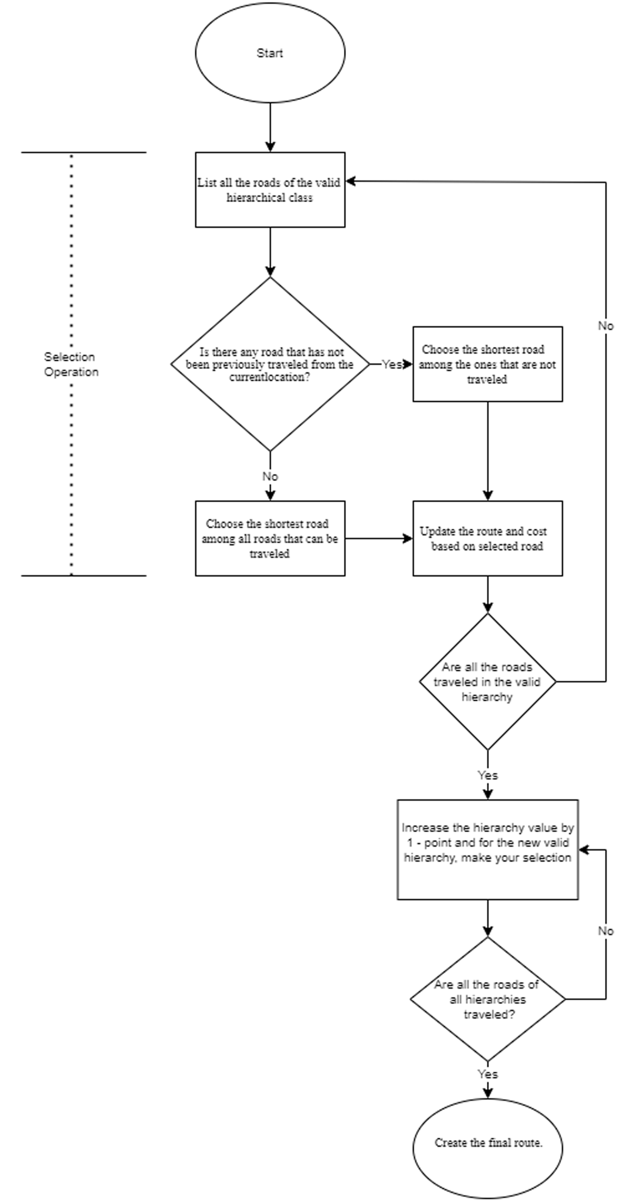
Flow chart of the heuristic algorithm.

3.2 Main steps of the proposed meta-heuristic algorithm

In this study, HCPP with Stochastic Travel Times (STT-HCPP), which is a new problem type, was taken into consideration. The proposed meta-heuristic algorithm was coded using the Matlab-2019b programming language.

Initial State: There are three parameters in the study that should be defined firstly: number of ants, number of iterations, and ant data table size.

The number of ants is one of the important parameters. More ants can deliver better outcomes and enhance the approach by increasing the chance. However, providing more ants raises the number of iterations, particularly in large-scale problems, causing the working period to be extended. According to the sensitivity analysis performed on the developed meta-heuristic, the number of ants was determined as 300. The number of iterations is the number of steps taken to obtain the optimum result. The low number of iterations might not be sufficient to achieve the outcome, but the high number of iterations often raises the calculation difficulties and thus, the working time [58]. According to the sensitivity analysis performed on the developed meta-heuristic, the number of iterations was determined as 1000. Besides, there is a visit matrix for each ant in the algorithm. This matrix of the visit indicates how many occasions the ant used a path on the routes it was traveling along. The general aim is to maintain these numbers in related visit data as low. As when we use these paths less, we will have the chance to keep the length of the route shorter. Unlike TSP, this new algorithm built for HCPP doesn’t depend on the amount of ant pheromone. In this type of problem, there is a possibility to cross a path more than one time. The usage aim of the algorithm’s visit data can be described as follows: reducing the cost, to prevent traveling at a constant local minimum.

There are two different route values of ants in the algorithm. The first of these is the general route. The general route is a path value that records the nodes the ant has visited beginning from the first node and following the rules of the hierarchy until it returns to the first node again. Another route value is the one in which the route of each hierarchy is recorded one by one.

Step 1. In the first iteration, each of the ants fills its visit matrix with “random choices, although it is likely to pursue the nearest node or the shortest path"

After the number of ants and iterations, the third parameter to be defined is the size of the ant data table. Two columns for each hierarchy are provided in the data table (1st hierarchy route is in the 1st column; while in the 2nd column, 1st hierarchy route length is provided). In the variable named “route capacity,” the value of rows in the table or how many ants’ data would be stored is established.

In the initial state, all data values were zero in the visit matrix since no location was visited. After the ant completes the whole path, a matrix is generated which is called “temporary visit data.”

Since there are 300 ants, there will be 300 matrices. These matrices are summed up with the mathematical logic and each value is divided by the number of ants to calculate the mean value for each path. With the equation below, in the temporary visit data matrix, we gathered the values for each ant.

$\begin{matrix} temporary visit data = temporary \\ visit data + k^{th} visit data; \end{matrix}$ (19)

The mean value of these 300 matrices was determined and reported at the end of the first iteration, as it is only applicable to the 1st iteration. Since we don’t have any other details on the visit because ants have not traveled them before. In other iterations, a ratio including the amount of evaporation or the coefficient of forgetting has been used. At this phase, 80% of the old mean data is taken and the 20% becomes evaporated, and the newest one is summed up with the mean value of the ants of that iteration and the mean value is measured. Therefore, both the past visit data were used, and the mean of the visit data obtained by the ant in this iteration was summed up and as a result, the mean of the values obtained was determined.

In this way; this data was also included in the arc data’s third element, which belongs to a 3-dimensional matrix, the first element being hierarchy values and the second element being distance/time values. With this step, we move to the 2nd iteration.

Step 2. (Selection process of the ant): The ant conducts the selection process in three different ways which are by looking at the routes in the database, looking at a single route, or looking at the visit data.

The Ant will start from the 1st node and will conduct step by step the procedures mentioned below. All of those procedures mentioned are repeated on every node in the same way. In a sense, a copy of the route database matrix is transmitted to the ant before beginning operations, which keeps all the good routes in the past.

1. Before making a selection when in the 1st or any node, it is initially tested at this moment if there are any other arcs in the hierarchy that have not been visited. If there is no arc, we move on without doing something, in other words, if all the paths in that hierarchy have been traveled, this time, the level of the ant’s arc, namely the level of the hierarchy it will traverse, would be increased by 1 point.

With this procedure, it is checked whether there is an arc that has not been traveled yet. If the ant is already in the max hierarchy and the arrived node is the first one, the ant has found a route and exits. If not, the arc level is increased by 1 point and the ant moves on to the next hierarchy. Furthermore, if the ant is in the max hierarchy and has not yet reached the first node even if it has traveled all the arcs, it can proceed to travel without doing anything as per the methods described below.

2. If it continues, it implies it also has to be navigated within the framework of the graph. Now it’s verified if there are any not visited arcs, on the condition that they’re in the same hierarchy. If any arcs are meeting this condition, only their list is recorded. In other words, if 1–3 arcs have been used before, this arc will not be included in the list. Only the list of unused arcs is included.

3. In the 3rd step, firstly, it is checked whether the ant is on the “new route” or not.

Selection by the database:

The “options” matrix is created for the possible targets that can be present in the second step. This matrix consists of 3 rows and n number of columns. The value n is the number of targets that are present in the second step. In the rows of the options matrix. In the first row, the possible targets that are present in the second step are provided, in the second row, the mean values of pheromones are stated, and in the third row, probability values are presented.

In this selection, the calculation of pheromones is performed as follows. The one with the best value (the lowest) among the shortest distance/time paths is selected from the node where the ant is placed and divided into a value such as 10000. The purpose of this step is to determine a value as the probability value. When the same procedure is finished with all the targets it can travel, the probability of choosing the path would rise with the higher value mentioned above.

Hereinafter, we can discuss the pheromone effect and distance effect parameters. As mentioned earlier, what is called the pheromone effect in this algorithm is essentially the effect of visit data, which is logically contrary to the pheromone effect in the ACO. However, it is called in the algorithm as a pheromone effect, just for the sake of clarity. The distance effect is the parameter that decides how the distance value would influence the likelihood of selecting the arc. Within the scope of the study, these values were regarded as Equation (20) and probability values are calculated using Equation (21). $pheromoneEffect = 4; distanceEffect = 0.3$ (20)

$\begin{matrix} Probability Value = {(\frac{1}{distance})}^{distanceEffect} \\ + {(\frac{1}{pheromoneMean})}^{pheromoneEffect} \end{matrix}$ (21)

Then the probability values are determined and the 3rd row of the matrix options are generated as well. Those probability values are normalized by leveling down to a value between 0–1. Then they are put on the roulette table when determining the value to be chosen, and a random number between 0–1 is obtained. This number is measured in terms of scale with the probability value, and the selection procedure is created accordingly.

After the node is selected, a different control mechanism is conducted. This control is about knowing whether there is another route in the database which matches the route generated after the target node has been selected.

By proceeding in this manner, eventually at some point, there will be only one route or no route will remain. If there is just one route remaining, the ant’s “one route” function is enabled, and the only path remaining is transferred to the ant from that database. After that, there will be no need to look at the database until you proceed to a new hierarchy.

Selection by single route:

If the ant follows this last remaining route, the probability to deviate from the route is modified. The brief checking takes place accordingly; “Should I select the next target on this one remaining route or should I quit this route?"

The probability of deviating from the route is determined as 0,003. A random number between the first node and the remaining number of nodes is determined up to 2 times the value of the remaining number of nodes in the test problems addressed within the scope of the research. This method aims to try to deviate as much as possible from a location to complete the route, that is to say, at least to follow a different path when the end of the route is attained. In this way;

If the value generated is less than or equivalent to 3, the target node is chosen in that single route as well as the single route is discarded. If abandoned, we will act with the visit data as we no longer have a database or route.

If the generated value is greater than 3, the only remaining route will be continued. Control is being performed by aiming the target and generating a random value again.

Selection based on visit data

Now we’ll look at the visit details as we get to the next method of selection. Yet again, as stated before, if there are nodes not chosen before and if all the nodes that the ant might go to have already been traveled, both of their list would appear in the matrix named “options”. In other terms, if there is even a single arc that was not previously used in that node, the arc is chosen without taking into consideration the arcs traveled before. No other negligence can be observed in probability calculations. But if there’s more than one unused arc, a selection is created among them this time. The previously visited arcs are not included in the process. Thus, irrespective of the selection process, the matrix of the target options to which the ant can go is established in this way. The four criteria listed below are used as per the visit data in the selection phase:

Alpha: It is the effect of the final pheromone (visit data) on the selection and its value is regarded as 0,7.

Beta: It is the coefficient that determines the effect of the arc length or cost on selection, and its value was calculated as 0,3.

Theta: The effect of the global pheromone (visit data) on the selection was regarded as 0,6.

Gamma: The effect value of the local pheromone (visit data) on the selection was regarded as 0,4.

The values calculated within the study scope are not of considerable significance, and their total is 1 because they are probabilities. Only theta must be selected as 0.6 since we seek to draw the best value to the global visit data. And the ant depends mostly on the memory of ants who completed their route.

There are two different visit data used here. The first of these, the global visit data, is the mutual matrix where the mean score of visit data of all ants is calculated and a certain amount of it becomes evaporated. The amount of local pheromone or visit data reflects the visit data obtained up to now by the current ant. Therefore, the ant focuses on both the number of instances itself used this path previously and how much it was used by other ants on average when deciding in this manner.

The final amount of pheromone (FAP) is the value to be derived from a calculation of the global and local visit data. The FAP and probability values of being selected are calculated as follows:

$\begin{matrix} FAP = (amount of local pheromone^{\land} gamma) * \\ (amount of global {pheromone}^{\land} theta) \end{matrix}$ (22) $value = ((1 / FAP)^{\land} alpha) * ((1 / distance)^{\land} beta)$ (23)

By evaluating the node choices from where the ant is positioned, according to the cases described above, the arc states of these nodes are determined with the variable named “value”. The probability of being chosen is then determined using these values and a random number between 0–1 is created by putting certain probability values on the roulette table using the same logic described in the previous sections. This probability value is taken into consideration and controlled and the selection is performed.

This is how the selection process ends. The node is chosen in three different ways which are by looking at the routes in the database, looking at a single route, or looking at the visit data.

Step 3. (Updates and ending): No matter how the node is chosen here, the following 3 procedures are applied:

The local visit data relating to the arc used by the ant (the matrix of the ant’s visit) is adjusted. The existing value is increased by 1 point to show that this arc has been used.

The overall distance to the ant travels and the present hierarchy road cost values are revised. The arc distance values which are used by the ant are added.

The selected node is added to the ant’s route.

The ant’s hierarchical route information passes through the following steps respectively. New information is added to the values which carry the best hierarchical routes in the matrix.

Firstly, it is checked whether the capacity of this table is full or not. In this way, how many routes the table will contain is determined in the algorithm by creating a variable called “route capacity”. If the route capacity has not been met yet, the ant’s hierarchical route data are respectively incorporated as it is.

If this route capacity is fulfilled, each hierarchical route of the ant is compared with the route costs that are listed in the table at the columns of that hierarchy. If it is better than any cost value, the route and cost value of the hierarchy we control of that ant is added instead of the worst (highest cost) route in the table. Then it proceeds to the other hierarchy route and that is checked as well. In this way, all hierarchy routes can be controlled.

With these procedures, the aim is to enable the table to maintain the best of each route of the hierarchy. These procedures are repeated after each ant completes its route. The iteration ends after all the ants finish their routes. At the end of the iteration, visit data are collected and updated. These procedures are carried out in the same way as defined in the preceding sections.

The algorithm’s pseudo code developed within the study scope and its detailed steps are shown in Algorithm 2.

Algorithm 2. Pseudo code of meta-heuristic algorithm
HN ← Number of hierarchies in the data set. h = 1,2,3,4,5 . . . ,HN
NN ← Total number of nodes in the data set
CM ← Cost / distance / time matrix between nodes
HM ← Dimensional matrix with the size of NNxNN that shows which hierarchy the roads between nodes have
VD (Visit Data) ← Matrix which has NNxNN dimensions to be allocated to each ant before initiating the route and with initial values as 0.
MVD (Mutual Visit Data) ← Matrix with dimensions of NNxNN which retains the visit data of ants that form a route in an iteration and whose values are reset if required after the iteration is completed.
GVD (General Visit Data) ← Matrix that has NNxNN dimensions and keeps the mean score of the ants’ past visit data.
GHR ← Table with column number of 2*HN, by acknowledging each hierarchy as different routes, the best of these routes their route distances are retained hierarchically that are received from the ants.
GBR ← Global Best Route (It represents the best route among all results until that moment.)
GBD ← Global Best Distance
k ← An empty ant object-sample
M = callfromFile();
fori = 1: NN
forj = 1: NN
value = CM [i,j]
end
end
For iter = 1:totalnumberofiterations
for antCount = 1:totalNumberofAnts
k ← Createant();
while true
if makekthchoice() = =- 1
break;
if kthrouteDistance > globalBestDistance>
GBR = kthRoute
GBD = kthrouteDistance
MVD = MVD+ kthVD
Forj = 1:HN
[hRoute, hCost] = kthhierarchyRoutes (h)
if GHR Findworse (hthRoute) = =true & &availableControl(hRoute)
Change (hRoute, hCost)
GVD = (GVD*Amountofevaporation + MVD/TotalNumberofAnts)/2
MVD = 0
Selection function for % ant
NTA(Not Traveled Arc)← It represents the arcs that the ant has not traveled before in the current hierarchy.
alpha ← Coefficient which is determining the effect of GVD and ant’s VD on mutual selection for a road.
beta ← Coefficient which is determining the effect of road length on selection
theta ← Coefficient which is determining the effect of the road between 2 nodes in GVD on the selection
gamma ← Coefficient which is determining the effect of the road between 2 nodes and the VD value of the ant on the selection NTA = FindnotvisitedArc(kthHN);
if NTA = =[] & &kthHN = =maxHierarchy & &kthlocation = =1
return -1;
else if NTA = =[] & &kthHN = maxHierarchy
kthHN = kthHN + 1;
else
NTA = FindnottraveledArc(kthHN);
if NTA = []
Options = NTA;
else
Options = Findarc(kthHN)
if (kthImonnewRoute = =false) & &isempty (kthsingleRoute)
fori = 1: length (options)
matchedRoute = min(GHR, [kthRoute + options (i)])
if matchedroute = 0
data (i) = 0;
else
data (i) = matchedRoute;
(data = =0)=0.0001 * min (data = 0);
selectedNode = rouletteSelection(options, data);
routes = control (GHR, [kthroute, selectedNode])
if length (routes) = =1
kthsingleRoute = routes;
else if length (routes) = =0
Imonkthnewroute = true;
elseif isempty (kthsingleRoute) = true
s→Deviation Rate
selectedNode = kthsingleRoute (1);
kthsingleRoute(1) = []
if generaterandomNumber ()<s
kthsingleRoute = [];
Imonkthnewroute = true;
Else // Decide Based On Visit Data
Options = Findarc(kthHN);
Fori = 1: length (options)
M1 = CM[kthLocation, options (i)]
X = kthVD[kthlocation, options (i)]
Y = GVD [kthlocation, options (i)]
ifX< = 0 & & Y = 0
Value (i) = ((1/M1)^∧beta);
elseifX< = 0 & & Y > 0
value (i)=(1/(Y^∧alpha)) * (1/(M1^∧beta));
elseifX > 0 & & Y > 0
value (i)=((1/(X^∧gamma * Y^∧theta))^∧alpha * (1/(M1^∧beta))
else
value(i)=((1/X)^∧alpha) * ((1/D1)^∧beta)
selectedNode = rouletteSelection(value);
kthroute = [kthroute, selectedNode]
kthrouteDistance = kthrouteDistance + CM [kthroute, selectedNode];
kthVD[kthlocation, selectedNode] + = 1;
return selectedNode;

Table 1

HCPP mathematical model, heuristic, and meta-heuristic approaches solution results

Name of the test problem	\|V\|	\|h\|	\| E\|	O ^Cplex	T^Cplex (s)	Gap (%)	O ^ACO	T^ACO (s)	O ^GSA	T^GSA (s)
Rnd_inst25	10	2	13	1281	0,94	0	1281	0,05	2422	0,08
Rnd_inst26	10	2	18	1417	483,28	0	1417	0,01	3687	0,01
Rnd_inst27	10	3	13	1386	32,14	0	1386	0,70	3762	0,02
Rnd_inst28	10	3	18	1516	124,25	0	1516	0,94	3226	0,04
Rnd_inst29	10	4	13	1249	2,02	0	1249	0,03	3400	0,01
Rnd_inst30	10	4	18	1582	65,34	0	1582	0,14	4210	0,03
Rnd_inst31	10	5	13	1013	0,77	0	1013	0,13	3978	0,20
Rnd_inst32	10	5	18	2006	182,53	0	2006	0,33	6397	0,02

Last but not least, distance values have been used directly for the HCPP solution in both algorithms in the objective function, but instead of the distance values for STT-HCPP, durations with defined mean and standard deviation values, which showed normal distribution characteristics have been used. Thus, the “random function” that generates random values for time values is applied in the algorithms.

4 Results

A sufficient amount of test problems was needed to test the heuristic and meta-heuristic algorithms of the STT-HCPP mathematical model which was presented in this study. The literature regarding HCPP has two small-sized test samples. Within the framework of this study, randomly generated test samples were mentioned in [14].

Considering a G = (V, E) graph, the test problems were stated as the set of nodes V = {10,20,30,40,50} and the set of hierarchies H = {2,3,4,5}. To assess the performance of the Cplex solver, the GSA-based heuristic and the ACO-based meta-heuristic were proposed comparatively and within the scope of the research, small-scale test problems were regarded as HCPP by considering the distances. Those examples were later modified to random travel times with normal distribution rather than the distances that are the study’s main subject. In these test problems, the distance values were transformed into time values based on the city’s legal speed limit. In algorithms, random time matrices were derived from defined mean and standard deviation values, and by using the suggested methods, solutions were pursued for test problems.

First, optimum findings were achieved by Cplex solver in General Algebraic Modeling System (GAMS) 24.2.3 for small-size problems by using HCPP mathematical model. These problems were the 13 and 18- edged test problems with 2,3,4, and 5 hierarchies while having 10 nodes. The maximum time to solve the aforementioned problems was determined as 1 hour (3600 seconds). Then the performance of the Cplex solver, the proposed GSA-based heuristic, and the ACO-based meta-heuristic was assessed comparatively with these results. The results are shown in Table 1.

The results that comparatively assess the performance of the Cplex solver, heuristic, and meta-heuristic approaches are in Table 1. In the problem solution, the results were obtained by using the Matlab-2019b program and a computer with 32 GB of memory and an Intel Core i9 9900K processor. In the first column of this table, the name of the test problem is given while in the second, third, and fourth columns, the number of nodes (|V|), the number of hierarchies (|h|), and the number of edges (|E|) of that problem are presented respectively. The fifth, sixth, and seventh columns describing the conclusions drawn from the Cplex solver indicate the best objective function value identified, the time of the computer solution, and the percentage difference between the best solution found by the Cplex solver and the best objective function value stated by Cplex. (O^Cplex, T^Cplex, Gap). While the eighth and ninth columns, showing the results obtained from the proposed ACO-based meta-heuristic approach, provide respectively the best objective function value (O^ACO) and the computer CPU time (seconds) of the best solution (T^ACO). Similarly, the tenth and eleventh columns showing the results obtained from the proposed GSA-based heuristic approach respectively present the best objective function value (O^GSA) and the computer CPU time (seconds) of the best solution (T^GSA).

The conditions for stopping the algorithms presented in this study were set as follows:

When the optimum solution is achieved in small-size problems,

For medium and large-sized problems, when the fixed number of iterations is reached, the algorithm termination process is performed.

Fig. 3

The objective function values for small-size HCPP.

For all 10-node, 13 and 18-edge problems; optimum solutions and routes were obtained in seconds/minutes with the Cplex solver and the proposed meta-heuristic. It was shown that with the suggested heuristic approach, those results were close to optimal. This is an expected result. Meta-heuristics perform better results than heuristics. Furthermore, these results are present in Fig. 3. When the computational times were evaluated, it was observed that the average score of computer CPU time used by the Cplex solver was 383 times higher than the suggested meta-heuristic, and the mean score of the computer CPU time used by the suggested meta-heuristic algorithm was 5,68 times higher than suggested heuristic. Thus, these three methods are successful at certain rates on these test problems. The results obtained regarding the computational times are in Fig. 4.

Fig. 4

Computational times for the small-size HCCP.

Tables 3 present the results obtained for STT-HCPP by using the algorithms created and the performance of the algorithms. In the first column of this table, the name of the test problem is given while in the second, third, and fourth columns, the number of nodes (|V|), the number of hierarchies (|h|), and the number of edges (|E|) of that problem are presented respectively. The fifth and sixth columns present respectively the best objective function value (O^ACO) obtained from the proposed ACO-based meta-heuristic approach and the computer CPU time (seconds) of the best solution (T^ACO). Similarly, the seventh and eighth columns showing the results obtained from the proposed GSA-based heuristic approach are respectively presenting the best objective function value (O^GSA) and the computer CPU time (seconds) of the best solution (T^GSA).

Table 2

Results of algorithms for instances with 10 and 20 nodes

Test Problems	\|V\|	\|h\|	\|E\|	O ^ACO	T^ACO (s)	O ^GSA	T^GSA (s)
Rnd_inst25	10	2	13	352,93	0,07	772,21	0,04
Rnd_inst26	10	2	18	382,44	0,23	866,87	0,01
Rnd_inst.annex1	10	2	30	625,66	3,98	1023,12	0,01
Rnd_inst27	10	3	13	393,09	0,18	1137,35	0,03
Rnd_inst28	10	3	18	410,59	5,16	942,59	0,01
Rnd_inst.annex2	10	3	30	643,76	5,72	1626,07	0,01
Rnd_inst29	10	4	13	362,71	0,31	1009,98	0,02
Rnd_inst30	10	4	18	418,11	0,60	1159,91	0,01
Rnd_inst.annex3	10	4	30	752,54	5,86	1512,15	0,01
Rnd_inst31	10	5	13	277,27	0,14	1135,04	0,02
Rnd_inst32	10	5	18	568,42	0,66	1652,14	0,02
Rnd_inst.annex4	10	5	30	758,23	5,40	2513,82	0,02
Rnd_inst33	20	2	55	1146,39	12,03	2441,45	0,04
Rnd_inst34	20	2	76	1658,10	1,871	2484,46	0,02
Rnd_inst.annex5	20	2	127	2329,00	12,67	4126,64	0,02
Rnd_inst35	20	3	55	1530,85	0,029	2259,77	0,02
Rnd_inst36	20	3	76	1674,52	11,49	3924,99	0,02
Rnd_inst.annex6	20	3	127	2466,04	15,15	5785,19	0,03
Rnd_inst37	20	4	55	1384,88	10,49	3795,34	0,03
Rnd_inst38	20	4	76	1708,00	11,37	5313,04	0,03
Rnd_inst.annex7	20	4	127	2721,70	15,43	7438,67	0,03
Rnd_inst39	20	5	55	1418,64	11,83	5436,73	0,12
Rnd_inst40	20	5	76	1821,66	13,48	4918,01	0,16
Rnd_inst.annex8	20	5	127	2632,03	16,02	8564,58	0,05

Table 3

Results of algorithms for instances with 30, 40, and 50 nodes

Test Problems	\|V\|	\|h\|	\|E\|	O ^ACO	T^ACO (s)	O ^GSA	T^GSA (s)
Rnd_inst41	30	2	125	2722,09	21,26	4821,46	0,05
Rnd_inst42	30	2	174	3434,05	99,91	5496,91	0,03
Rnd_inst.annex9	30	2	290	5802,46	49,71	9330,78	0,04
Rnd_inst43	30	3	125	2831,39	20,05	6515,62	0,04
Rnd_inst44	30	3	174	3791,72	33,71	6951,35	0,03
Rnd_inst.annex10	30	3	290	5939,79	33,29	12939,8	0,04
Rnd_inst45	30	4	125	2888,26	22,19	8046,46	0,03
Rnd_inst46	30	4	174	4139,53	28,40	10155,04	0,05
Rnd_inst.annex11	30	4	290	6165,37	40,24	13162,52	0,05
Rnd_inst47	30	5	125	3557,33	24,65	11733,46	0,05
Rnd_inst48	30	5	174	4050,81	28,64	13744,53	0,04
Rnd_inst.annex12	30	5	290	6656,80	35,87	23174,55	0,07
Rnd_inst49	40	2	223	4555,29	879,91	20488,21	0,25
Rnd_inst50	40	2	312	6381,16	39,54	10347,59	0,09
Rnd_inst.annex13	40	2	520	10015,17	94,71	17383,74	0,10
Rnd_inst51	40	3	223	5338,09	35,11	10404,01	0,14
Rnd_inst52	40	3	312	6500,28	108,63	13902,66	0,11
Rnd_inst.annex14	40	3	520	10528,82	64,94	22885,18	0,12
Rnd_inst53	40	4	223	5537,26	42,68	15607,80	0,13
Rnd_inst54	40	4	312	7655,61	53,73	15705,82	0,12
Rnd_inst.annex15	40	4	520	10939,70	187,26	27905,17	0,16
Rnd_inst55	40	5	223	6148,42	41,28	19498,20	0,19
Rnd_inst56	40	5	312	7766,13	48,61	23646,31	0,17
Rnd_inst.annex16	40	5	520	11776,57	78,08	35088,12	0,19
Rnd_inst57	50	2	350	7322,92	99,26	10628,49	0,09
Rnd_inst58	50	2	490	9513,57	896,83	14235,58	0,10
Rnd_inst.annex17	50	2	817	15671,36	667,35	23720,74	0,17
Rnd_inst59	50	3	350	7935,79	119,30	18032,64	0,17
Rnd_inst60	50	3	490	10710,27	72,16	18779,64	0,15
Rnd_inst.annex18	50	3	817	16414,84	150,80	28182,93	0,16
Rnd_inst61	50	4	350	8669,10	63,84	23577,02	0,18
Rnd_inst62	50	4	490	11633,40	73,47	31106,80	0,20
Rnd_inst.annex19	50	4	817	17155,59	108,33	44820,77	0,22
Rnd_inst63	50	5	350	9572,20	73,16	22751,62	0,19
Rnd_inst64	50	5	490	12434,50	76,82	37097,74	0,22
Rnd_inst.annex20	50	5	817	17939,30	198,57	47792,28	0,24

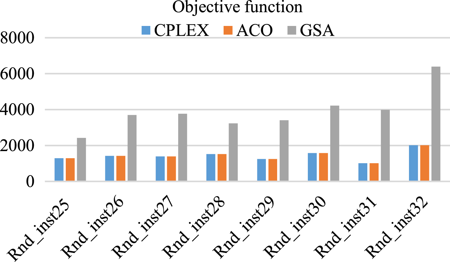
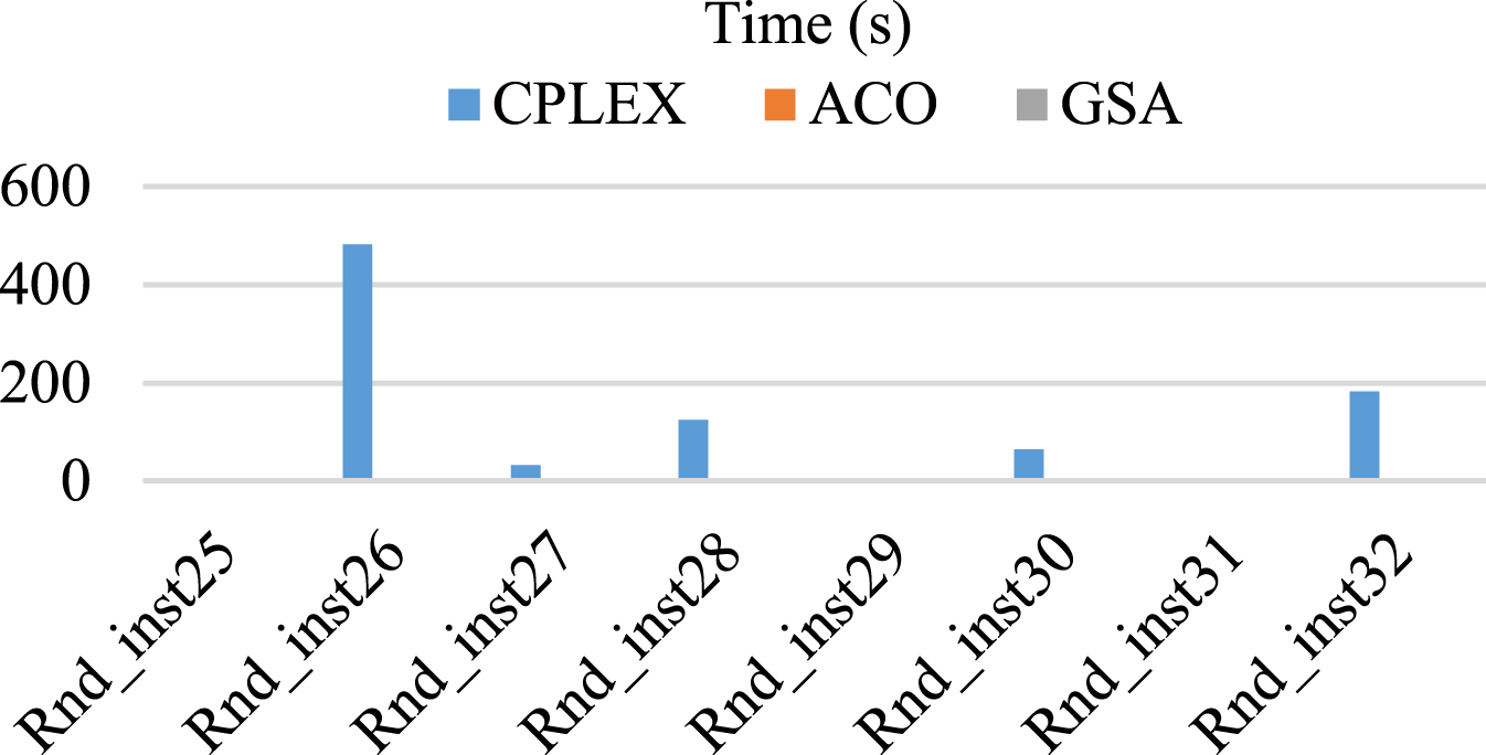
In all instances with 10 and 20 nodes, the ACO-based meta-heuristic approach found better objective function values than the GSA-based heuristic approach. In these problems, the average best objective function value found by the GSA-based heuristic was 2.44 times higher than the average best objective function value found by the ACO-based meta-heuristic. However, it was seen that the heuristic algorithm gives better results as the number of edges increases For example, for Rnd_inst25 with 10 nodes and 13 edges, the value of the objective function found by the heuristic was 2.19 times higher than the value of the objective function of the meta-heuristic; for Rnd_inst.annex1 with 10 nodes and 30 edges, the value of the objective function the heuristic finds was 1.64 times higher than the value of the objective function of the meta-heuristic. Although the ACO-based meta-heuristic algorithm finds better results in all of these test instances, the average time used by the ACO-based meta-heuristic algorithm was 204 times larger than the GSA-based heuristic. However, the average time used by ACO was less than 1 minute in all of these test instances. The average time used by GSA was less than 1 second. This shows that the algorithms are performing well.

As the problem size in STT-HCPP increases, the complexity of the network increases, and thus the time in both approaches for the solution increases. For example, network representations of Rnd_inst25 and Rnd_inst.annex20 are represented in Fig. 5.

Fig. 5

Hierarchical network of instances (a) for Rnd_inst25; (b) for Rnd_inst.annex20.

For the test problems discussed within the scope of the study, average objective function values, and computational times are in Figs. 6 7 respectively.

In short, a chance-constrained stochastic programming approach was used in this study to account for the uncertain environment of the traffic situation in HCPP which was caused by various factors (varying traffic density, weather conditions, environmental conditions such as accidents and roadworks, etc). In the HCPP mathematical model, the c_ij coefficients were considered as parameters with normal distribution, and STT-HCPP emerged, which better meets real-life problems. In this model, deterministic objective function E(z) with the expected value model was used. In the study, starting from instances having 10 nodes, 13 arcs and 2 hierarchies up to having 50 nodes,817 arcs and 5 hierarchies, total of 60 test instances have been solved. In the solution of large-sized problems (as many as 817 edges), two approaches have been proposed to reach the solution. As can be seen from the results, the proposed effective algorithms give good results in seconds/minutes for this arc routing problem with the NP-hard problem class. The results show that the proposed approaches perform well. While a general-purpose solver like General Algebraic Modeling System (GAMS) cannot provide a solution for instances with more than 10 nodes, the methods suggested in the study yielded results within seconds/minutes, even for instances having 50 nodes, 817 arcs and 5 hierarchies. Also, a sensitivity analysis was performed for the ACO-based meta-heuristic algorithm.

4.1 Sensitivity analysis

Sensitivity analyses were performed on the developed ACO-based meta-heuristic according to different ant number and iteration number parameters. A sensitivity analysis was conducted to show the changes in the main output related to the changes in different important parameters [42]. This analysis was performed for all test problems. As an example, results were provided for Rnd_inst61 with 50 nodes and 350 edges. The sensitivity is depicted in Fig. 8 and Fig. 9. In Fig. 8, assuming the ant number along the horizontal axis and the objective function value (O^GSA) along the vertical axis, and in Fig. 9, taking the horizontal axis as the iteration number and the vertical axis as the objective function value (O^GSA); two different graphs are plotted.

Fig. 6

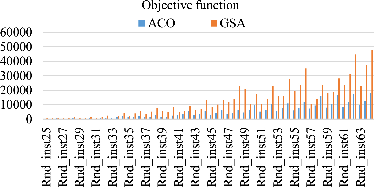
The objective function of the suggested algorithms.

Fig. 7

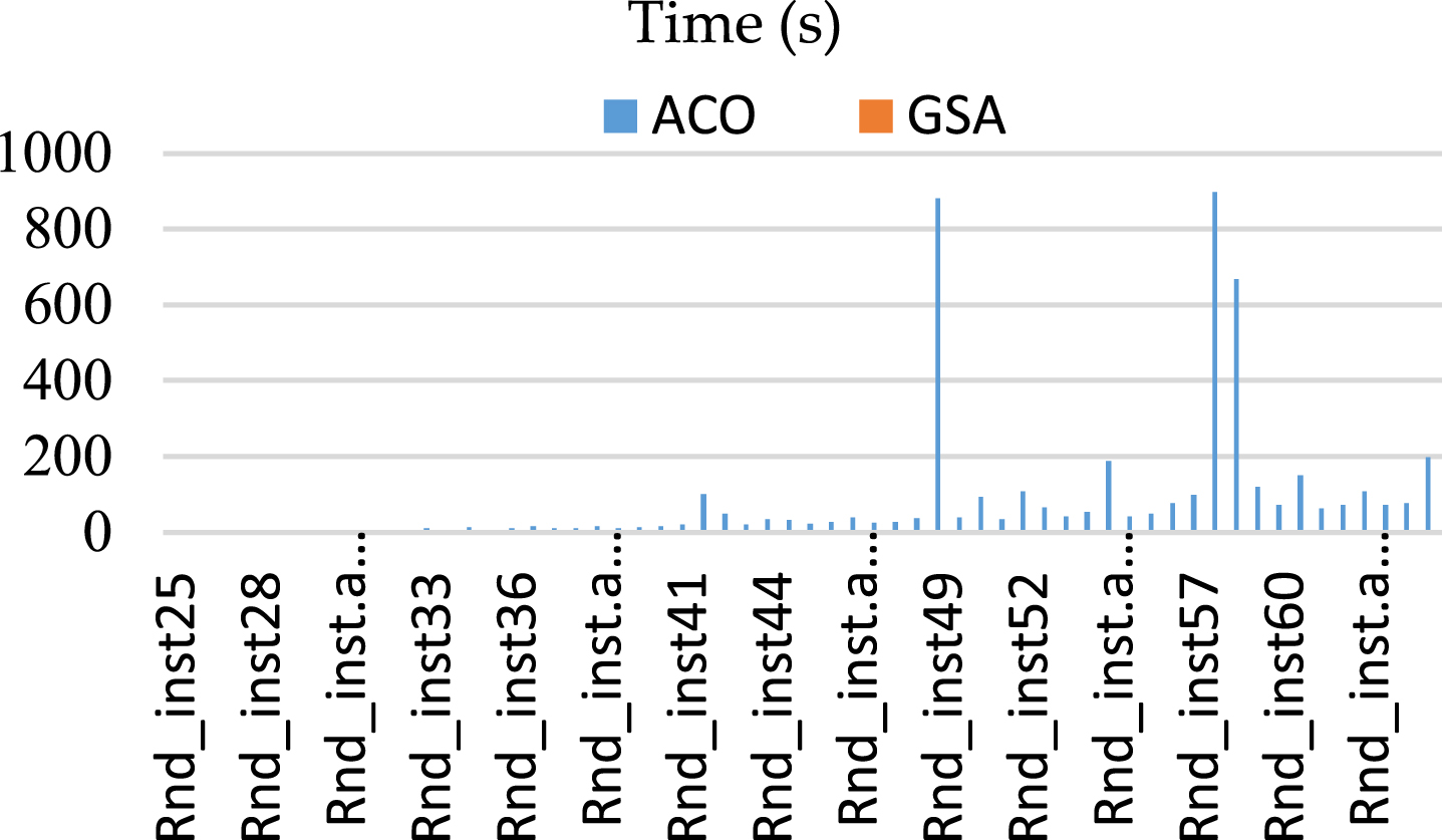
Computational times for the suggested algorithms.

Fig. 8

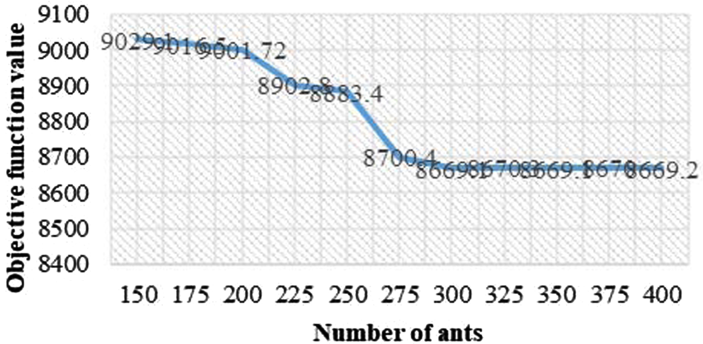
The sensitivity analysis results for the number of ants.

Fig. 9

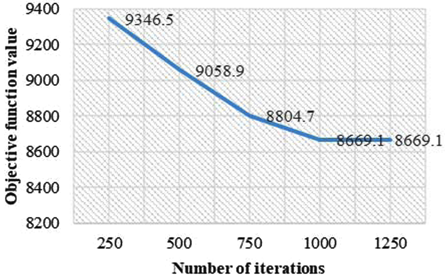
The sensitivity analysis results for the number of iterations.

Here, the change in the objective function was observed by changing the ant number parameter between 150 and 400 and the iteration number parameter between 250-1250. It can be noticed from Fig. 8 that keeping the ant count constant at 300 provides the best cost for Rnd_inst61. At this point (O^GSA) remains almost the same. Likewise, as can be seen in Fig. 9, the best cost value was obtained since the number of iterations was set to 1000.

5 Conclusion and future work

Although there are wide application areas such as street sweeping, garbage collection and snow removal in real life; HCPP has been the subject of research with a limited number of studies for about 35 years. In this study, a new problem type namely the STT-HCPP was presented. In many other HCPP studies in the literature, attention was given to the distance traveled by the vehicles throughout the routing. That being said, in today’s modern world in which the competition in the market is at its height, identifying the travel times between nodes is necessary in order not to waste time and execute the planning process accurately. In most real-life issues, due to unpredictable weather conditions, environmental factors, or changing traffic density, it is not always possible to express the travel times and speed with exact values. Although the travel times depend on the distance, on the very same day, it may be stochastic due to incidents or various factors that obstruct travel. Owing to this uncertainty, HCPP has been solved within the scope of this paper using the chance-constrained stochastic programming method. The stochastic analysis of travel times is significant in terms of meeting real-life situations. The objective function coefficients which constitute the randomness in the chance-constrained model are supposed to be compliant with a normal distribution. The suggested model was only able to find a solution for small-sized samples due to the NP-hard nature of the problem. Two new approaches, one of which is heuristic and the other meta-heuristic, were proposed through the use of Matlab-2019b programming language to solve sixty test instances addressed in the purview of the research to identify solutions on the proper time to medium and large problems. The suggested algorithms were tested by using the test problems and their effectiveness was compared. The algorithms suggested on the basis of these results offer suitable solutions in a short time, including for large-size problems. As can be seen in Tables 1 –3; although the ACO-based meta-heuristic algorithm returns better results in all test instances, the average time used by the GSA-based heuristic is less than the ACO-based meta-heuristic algorithm. These results are presented in Figs. 6 7. One possible explanation for this is that the meta-heuristic, unlike the heuristic, searches all space for the solution. Finally, the sensitivity of the meta-heuristic is analyzed based on the number of ants and the maximum number of iterations. It is aimed that the introduced problem type will be easier to adapt to real life due to the uncertainty involved and the proposed stochastic-based solution methods will be the first in the literature.

For further research, several examples can be illustrated. It is appropriate to discuss cases in which stochastic travel times suit various distributions (such as triangular, gamma, etc.). The meta-heuristic algorithm established can be evaluated under various parameter values. Different heuristic and/or meta-heuristic approaches can be developed for STT-HCPP. The solutions obtained can be compared with the ones obtained in this study.

References

Corberan

, Marti

and Sanchis

J.M.

, A grasp heuristic for the mixed Chinese postman problem, European Journal of Operational Research 142 (2002), 70–80.

Kao

E.P.C.

, A preference order dynamic program for a stochastic traveling salesman problem, Operations Research 26 (1978), 1033–1045.

Tas

, Dellaert

, Van Woensel

and De Kok

, Vehicle routing problem with stochastic travel times including soft time windows and service costs, Computers & Operations Research 40 (2013), 214–224.

Tadei

, Perboli

and Perfetti

, The multi-path traveling salesman problem with stochastic travel costs, EURO Journal on Transportation and Logistics 6 (2017), 3–23.

Dror

, Stern

and Trudeau

, Postman tour on a graph with precedence relation on arcs, Networks 17 (1987), 283–294.

Alfa

A.S.

and Liu

D.Q.

, Postman routing problem in a hierarchical network, Engineering Optimization 14 (1988), 127–138.

Damodaran

, Krishnamurthi

and Srihari

, Lower bounds for hierarchical Chinese postman problem, International Journal of Industrial Engineering: Theory, Applications and Practice 15 (2008), 36–44.

Ghiani

and Improta

, An algorithm for the hierarchical Chinese postman problem, Operations Research Letters 26 (2000), 27–32.

Cabral

E.A.

, Gendreau

, Ghiani

and Laporte

, Solving the hierarchical Chinese postman problem as a rural postman problem, European Journal of Operational Research 155 (2004), 44–50.

10.

Korteweg

and Volgenant

, On the hierarchical Chinese postman problem with linear ordered classes, European Journal of Operational Research 169 (2006), 41–52.

11.

, Viriyasuthee

and Rekleitis

, Efficient complete coverage of a known arbitrary environment with applications to aerial operations, Autonomous Robots 36 (2014), 365–381.

12.

Sayata

U.B.

and Desai

N.P.

, (12-13 June 2015). An algorithm for Hierarchical Chinese postman problem using minimum spanning tree approach based on Kruskal’s algorithm, IEEE International Advance Computing Conference (IACC), Banglore, India.

13.

Colombi

, Corberan

, Mansini

, Plana

and Sanchis

J.M.

, The hierarchical mixed rural postman problem: polyhedral analysis and a branch-and-cut algorithm, European Journal of Operational Research 257 (2017), 1–12.

14.

Kayacı Çodur

and Yılmaz

, A time-dependent hierarchical Chinese postman problem, Central European Journal of Operations Research 28 (2020), 337–366.

15.

Tan

, Cui

and Zhang

, (23-28 October 2005). Chinese postman problem in stochastic networks. In Joint International Conference on Autonomic and Autonomous Systems and International Conference on Networking and Services-(icas-isns’ 05), Papeete, Tahiti, French Polynesia.

16.

Zhang

and Peng

, Uncertain programming model for Chinese postman problem with uncertain weights, Industrial Engineering & Management Systems 11 (2012), 18–25.

17.

Majumder

, Kar

and Pal

, Uncertain multi-objective Chinese postman problem, Soft Computing 23 (2019), 11557–11572.

18.

Carraway

R.L.

, Morin

T.L.

and Moskowitz

, Generalized dynamic programming for stochastic combinatorial optimization, Operations Research 37 (1989), 819–829.

19.

Laporte

, Louveaux

and Mercure

, The vehicle routing problem with stochastic travel times, Transportation Science 26 (1992), 161–170.

20.

Kenyon

A.S.

and Morton

D.P.

, Stochastic vehicle routing with random travel times, Transportation Science 37 (2003), 69–82.

21.

Kim

, Lewis

M.E.

and White

C.C.

, Optimal vehicle routing with real-time traffic information, IEEE Transactions on Intelligent Transportation Systems 4 (2005), 178–188.

22.

Jula

, Dessouky

and Ioannou

, Truck Route Planning in Non-Stationary Stochastic Networks with Tine-Windows at Customer Locations, IEEE Transactions on Intelligent Transportation Systems 37 (2006), 51–63.

23.

Russell

R.A.

and Urban

T.L.

, Vehicle routing with soft time windows and Erlang travel times, Journal of the Operational Research Society 59 (2008), 1220–1228.

24.

Chang

, Wan

and Tsang

, A stochastic dynamic traveling salesman problem with hard time Windows, European Journal of Operational Research 198 (2009), 748–759.

25.

Shen

, Ordóñez

and Dessouky

, The stochastic vehicle routing problem for minimum unmet demand. In Optimization and logistics challenges in the enterprise, W. Chaovalitwongse., K. C. Furman., P. M. Pardalos., Eds.; In Springer Optimization and Its Applications, Springer: Boston, US. 2009; volume 30, pp. 349–371.

26.

Hou

and Zhou

, (28-31 May 2010). Stochastic vehicle routing problem with uncertain demand and travel time and simultaneous pickups and deliveries. 2010 Third International Joint Conference on Computational Science and Optimization, Huangshan, Auhui, China.

27.

, Tian

and Leung

S.C.

, Vehicle routing problems with time windows and stochastic travel and service times: Models and algorithm, International Journal of Production Economics 125 (2010), 137–145.

28.

Errico

, Desaulniers

, Gendreau

, Rei

and Rousseau

L.M.

, The vehicle routing problem with hard time windows and stochastic service times, EURO Journal on Transportation and Logistics 7 (2016).

29.

Zhang

, Lam

W.H.

and Chen

B.Y.

, A stochastic vehicle routing problem with travel time uncertainty: trade-off between cost and customer service, Networks and Spatial Economics 13 (2013).

30.

Errico

, Desaulniers

, Gendreau

, Rei

and Rousseau

L.M.

, A priori optimization with recourse for the vehicle routing problem with hard time windows and stochastic service times, European Journal of Operational Research 249 (2016), 55–66.

31.

Gutierrez

, Dieulle

, Labadie

and Velasco

, A multi population memetic algorithm for the vehicle routing problem with time windows and stochastic travel and service times, IFAC-Papers OnLine 49(12) (2016), 1204–1209.

32.

Ehmke

J.F.

, Campbell

A.M.

and Urban

T.L.

, Ensuring service levels in routing problems with time windows and stochastic travel times, European Journal of Operational Research 240 (2015), 539–550.

33.

Binart

, Dejax

, Gendreau

and Semet

, A 2-stage method for a field service routing problem with stochastic travel and service times, Computers & Operations Research 65 (2016), 64–75.

34.

Miranda

D.M.

and Conceicão

S.V.

, The vehicle routing problem with hard time windows and stochastic travel and service time, Expert Systems with Applications 64 (2016), 104–116.

35.

Nguyen

V.A.

, Jiang

, Ng

K.M.

and Teo

K.M.

, Satisficing measure approach for vehicle routing problem with time windows under uncertainty, European Journal of Operational Research 248 (2016), 404–414.

36.

Miranda

D.M.

, Branke

and Algorithms

S.V.

, for the multi-objective vehicle routing problem with hard time windows and stochastic travel time and service time, Applied Soft Computing 70 (2018), 66–79.

37.

Mukherjee

, Panigrahi

, Kar

and Maiti

, Constrained covering solid travelling salesman problems in uncertain environment, Journal of Ambient Intelligence and Humanized Computing 10 (2019), 125–141.

38.

Majumder

, Kundu

, Kar

and Pal

, Uncertain multi-objective multi-item fixed charge solid transportation problem with budget constraint, Soft Computing 23 (2019), 3279–3301.

39.

Dutta

, Barma

P.S.

, Kar

and De

, A modified kruskal’s algorithm to improve genetic search for open vehicle routing problem, International Journal of Business Analytics (IJBAN) 6 (2019), 55–76.

40.

Ulmer

M.W.

, Goodson

J.C.

, Mattfeld

D.C.

and Thomas

B.W.

, On modeling stochastic dynamic vehicle routing problems, EURO Journal on Transportation and Logistics 9 (2020), 100008.

41.

Bakach

, Campbell

A.M.

, Ehmke

J.F.

and Urban

T.L.

, Solving vehicle routing problems with stochastic and correlated travel times and makespan objectives, EURO Journal on Transportation and Logistics 10 (2021), 100029.

42.

Barma

P.S.

, Dutta

, Mukherjee

and Kar

, A hybrid GA-BFO algorithm for the profit-maximizing capacitated vehicle routing problem under uncertain paradigm, Journal of Intelligent &Fuzzy Systems 40 (2021), 8709–8725.

43.

Keenan

, Panadero

, Juan

A.A.

, Martí

and McGarraghy

, A strategic oscillation simheuristic for the time capacitated arc routing problem with stochastic demands, Computers & Operations Research 133 (2021), 105377.

44.

Müller

J.P.

, Elbert

and Emde

, Integrating vehicle routing into intermodal service network design with stochastic transit times, EURO Journal on Transportation and Logistics 10 (2021), 100046.

45.

Jie

K.W.

, Liu

S.Y.

and Sun

X.J.

, A hybrid algorithm for time-dependent vehicle routing problem with soft time windows and stochastic factors, Engineering Applications of Artificial Intelligence 109 (2022), 104606.

46.

Liu

, Li

and Khojandi

, The flying sidekick traveling salesman problem with stochastic travel time: A reinforcement learning approach, Transportation Research Part E: Logistics and Transportation Review 164 (2022), 102816.

47.

Atalay

K.D.

and Apaydın

, Şans kısıtlı stokastik programlama problemlerinin deterministik eşitlikleri, Anadolu Universitesi Bilim ve Teknoloji Dergisi 1 (2011), 1–18.

48.

Higle

J.L.

, Stochastic programming: Optimization when uncertainty matters. In Emerging Theory, Methods, and Applications; Informs: Catonsville, MD, USA, 2005. pp. 30–53.

49.

Gendreau

, Laporte

and Séguin

, Stochastic vehicle routing, European Journal of Operational Research 88 (1996), 3–12.

50.

Oyola

, Arntzen

and Woodruff

D.L.

, The stochastic vehicle routing problem, a literature review, part I: models, EURO Journal on Transportation and Logistics 7 (2018), 193–221.

51.

Pramanik

, Jana

D.K.

, Mondal

S.K.

and Maiti

, A fixed-charge transportation problem in two-stage supply chain network in Gaussian type-2 fuzzy environments, Information Sciences 325 (2015), 190–214.

52.

Charnes

and Cooper

W.W.

, Chance-constrained programming, Management Science 6(1) (1959), 73–79.

53.

Taha

H.A.

, Operations Research an Introduction. 7th ed.; Prentice Hall, NJ, United States. 2007.

54.

Aksaraylı

and Pala

, Şans kısıtlı stokastik programlama yaklaşımı ile ofis ürünleri üretim sistemi modellemesi. 15. Üretim Araştırmaları Sempozyumu 2015.

55.

Hulsurkar

, Biswal

M.P.

and Sinha

S.B.

, Fuzzy programming approach to multi–objective stochastic linear programming problems, Fuzzy Sets and Systems 88 (1997), 173–181.

56.

Yılmaz

, Route management for vehicles used in road maintenanceactivities through hierarchical Chinese postman problem approach, Journal of the Institute of Science and Technology 8(2018), 107–115.

57.

Dorigo

and Socha

, An introduction to ant colony optimization, IRIDIA, Bruxelles, technical report series 2007.

58.

Kapukaya

, Design of self tuning pid controller using adaptive particular swarm optimization and ant colony optimization (M.Sc. Thesis), Kahramanmaras Sştçü Imam University, Kahramanmaras, 2019.