Multivariate time-series anomaly detection via temporal convolutional and graph attention networks

Abstract

Multivariate time series anomaly detection has been investigated extensively in recent years. Capturing long-term time series information is one of the challenges in this field. We propose a novel multivariate time series anomaly detection framework MTAD-TCGA comprising several modules that efficiently and accurately capture dependencies in long-term multivariate time series. The proposed model contains a temporal convolutional module and uses two parallel graph attention layers to learn the complex dependencies of time series in both the temporal and feature dimensions. A Gated Recurrent Unit layer, based on an improved attention mechanism, and an auto-regressive model is used for prediction, and the prediction model and reconstruction model are jointly optimized. Finally, the threshold is selected by extreme value theory, and then anomalies are identified. The experimental results on three public datasets show our framework is superior to other state-of-the-art models, achieving F1 scores uniformly at levels above 0.9, verifying the effectiveness and feasibility of the MTAD-TCGA method.

Keywords

Long-term time series anomaly detection time convolution network graph attention network gated recurrent unit

1 Introduction

Time series data [12] are among the most common data types; the term refers to an ordered dataset obtained by sampling the same indicators in chronological sequence. Time series data are ubiquitous in many fields of study, so analysis and research on time series data is extensive, historically and currently. In analyzing time series, isolating data anomalies is critical; they must be either rejected or treated differently. Anomaly detection [26] of time series data [7] finds the samples that have obvious differences from normal samples; it is presently an important research topic. Anomaly detection in multivariate time-series is of great significance in machine learning and has a wide range of applications in industry [17], in financial transactions and in medical fields [11], and so on. Efficient and accurate anomaly detection helps organizations to monitor their key metrics continuously and receive timely alerts for potential incidents [14].

It remains a significant challenge to capture long-term time series information because of its complex characteristics, such as unevenness, time dependencies, and randomness. Recurrent neural networks (RNN) [20] serve as a starting point for modeling temporal dependencies in deep learning, and traditional RNN still has difficulty capturing long temporal dependencies due to gradient disappearance. Long Short-Term Memory (LSTM) [32] and Gated Recursive Unit (GRU) [18], which are its variants, mitigate this limitation by introducing a gate design. The attention mechanism has also become widely used to model temporal patterns of time series data because of its ability to focus on particular timestamps. As a result, GRU models based on the attention mechanism were proposed and used for time series anomaly detection, showing good performance in modeling temporal correlation.

Recently, graph networks have become popular in time series analysis, and many models use graph attention mechanisms to model the relationship between variables. One of the very good methods is MTAD-GAT, which was first proposed in 2020 [15]. It utilizes two graph attention mechanisms to simultaneously and comprehensively model the correlation between variables both over time and among the features of the multiple variables; it considers errors from both prediction and reconstruction perspectives and achieves high accuracy. Most graph-based models have performed well modeling correlations between different features in time series data, but research reported since the seminal 2020 proposal of MTAD-GAT has not, in our opinion, sufficiently treated the difficult problem of modeling long-term information in multivariate time series analysis; such consideration and attention in the research will improve data prediction and anomaly detection.

In order to better model the long-term time series dependencies of the data, this paper proposes a novel architecture MTAD-TCGA that first uses a Temporal Convolutional Network (TCN) specialized in long time series to extract features from the data, and then uses a time-based Graph Attention Network (GAT) and a GRU based on a temporal Gaussian kernel attention mechanism to jointly capture the series’ temporal information.

In contrast to most graph-based models, which would ignore the dependencies among modeled times, our architecture integrates both temporal and feature dimensions to model the complex dependencies of the data from two perspectives. As is MTAD-GAT, the whole process is modeled from both prediction and reconstruction perspectives, but to further simplify the model and improve its robustness, an auto-regressive (AR) model is added to the prediction to jointly, with the neural network, predict the time series data. The AR model improves the performance of the model at a different time scale than the deep learning model. The model is moderately simplified by replacing the variational self-encoder with an RNN decoder in the reconstruction module.

The principal contributions of this paper are as follows:

Modules such as TCN, GAT, and GRU are combined to model the correlation between multiple timestamps and better capture the long-term temporal dependencies of the data.

We propose a GRU-Attention layer based on the Gaussian kernel, and the Gaussian kernel function is used to focus the timestamp again to improve the accuracy of the model.

Based on integrated learning theory, a statistical auto-regressive model is parallelized with a neural network to reduce the complexity of the model and further improve its robustness.

The remainder of this paper is organized as follows:

Section 2 outlines some methods for time series anomaly detection. Section 3 discusses the details of the MTAD-TCGA model. Section 4 provides the experimental setups and discusses the results. Section 5 presents the conclusions.

2 Related work

Some common traditional methods for time series anomaly detection are 3-Sigma criterion, Boxplot method, Auto-Regressive Integrated Moving Average model (ARIMA) [19], and Local Outlier Factor algorithm (LOF) [2], which take the samples that deviate from the overall distribution as anomalies; they are classical probabilistic statistical models [27]. Li Quan et al. proposed an anomaly detection algorithm based on Kernel Principal Component Analysis (KPCA) [24]. Their kernel function can map the data to a high-dimensional space but avoids dimensional disasters. Their model combines the kernel function with principal component analysis to jointly process the data features, but the kernel function in Li Quan’s method has too large an impact on the detection results and the algorithm is less efficient.

Research developments during the ‘big data’ era found that deep learning is more suitable for handling large-scale complex data than traditional statistical methods. Several deep learning methods have been proposed in the literature for time series anomaly detection, based on progress in the field of deep learning, presented in the representative published works.

LSTM-VAE [8], which was proposed in 2017, is a variational self-encoder based on long and short-term memory; the model fuses variables and reconstructs the expected distribution of variables. In the encoding process, the method applies LSTM and VAE [9, 10] to project the time-series data of multiple variables into the hidden space, and the decoding process estimates a potential representation of the expected distribution of the multivariate input. The model performs very well on multiple datasets. In 2018, Kyle et al. [23] proposed the LSTM-NDT model, a dynamic unsupervised anomaly detection method without parameter threshold selection, which also proposed a pruning strategy to reduce the false alarm rate. In the same year, Zong et al. [5] proposed the DAGMM model for unsupervised anomaly detection, which combined self-encoder with the Gaussian model and achieved good results. In 2019, Ya Su [35] proposed OmniAnomaly, a stochastic model constructed to capture the normal patterns behind multivariate time series data by learning feature representations. The algorithm is to some extent able to find the variables that cause the appearance of anomalies and propose an explanation for the occurrence of the anomaly.

In 2020 and 2021, USAD [16] and DAEMON [34] combined self-encoder and GAN structures to find anomalies by reconstructing the original input data. Recently, graph neural networks (GNN) [25], including graph convolution networks (GCN) [33], graph attention networks (GAT) [30], and so on, have shown great success in modeling various types of data. The framework MTGNN [36], which was proposed in 2020 to incorporate GNN, learns one-way relationships between variables through graph learning modules, to better capture the dependencies in multivariate data. In the same year, Hang Zhao et al. [15] proposed the MTAD-GAT algorithm, which uses two parallel GATs to process the time and feature data separately, achieving better accuracy; the paper is also the main reference of this paper, which establishes an improvement to the MTAD-GAT method. In 2021, Ailin Deng et al. [1] proposed a Graph Deviation Network, or GDN, that uses a Graph Neural Network (GNN) to learn the relationship between variables and enhances the interpretability of the model. Since the publication of MTAD-GAT, Transformer and subsequent variations, including the Anomaly Transformer model [21] proposed by Xu in 2022, have also made great progress in many fields. Xu’s model draws on self-attention to perform correlation modeling on time series, and applies Transformer to time series anomaly detection.

The performance of these existing methods in detecting anomalies in multivariate time series is still unsatisfactory due to the difficulty of capturing the long-term time dependence of time series data and variable correlations, we propose MTAD-TCGA, which overcomes these difficulties.

3 Proposed framework

3.1 Problem statement

This paper focuses on multivariate time series anomaly detection. A set of time series data X = {x₁, x₂, …, x_T} is given, in which T is the length of the input window and the samples are multivariate at dimension k. We predict the future data in a rolling way; for example, the value of x_T+1 is predicted through x₁, x₂, …, x_T. The problem under study is written as follows: the input matrix is X = {x_t-T, x_t-T+1, …, x_t-1} ∈ R^k×T, the prediction is y_t, and finally, a threshold is selected to find the abnormal samples.

3.2 Overview

To further improve the modeling of long-term dependencies in time series, a novel multivariate time series anomaly detection model MTAD-TCGA is constructed. Its overall network architecture is shown in Fig. 1 and it comprises the following modules.

Feature extraction is performed first using the TCN, where the design of the dilated causal convolution in the TCN module allows for better extraction of longer time series features.

The processed data is delivered to two parallel graph attention (GAT) layer; one applies the attention mechanism to the multi-variate features, and the other applies it to the time dimensions, thus focusing on particular features and timestamps.

The outputs of the TCN layer and the two GAT layers are concatenated and fed to a GRU layer with kernel attention, which continues to capture the sequential patterns in the time series.

An AR model is parallelized with a neural network to reduce model complexity; the prediction-based model and the reconstruction-based model joint optimize by together defining the model error.

The Peaks Over Threshold (POT) method is used to analyze the prediction and reconstruction errors of the model, obtaining the threshold value and improving the anomaly detection accuracy.

Fig. 1

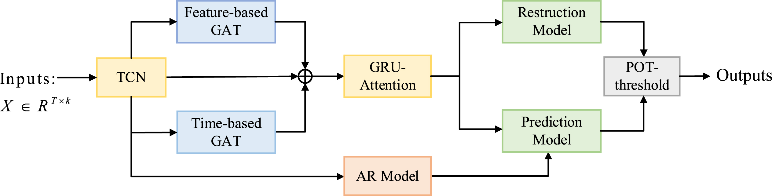
Overall structure of MTAD-TCGA.

3.3 Data preprocessing

Since the variable sets in different datasets are different, the dimensions of the data are generally different. In order to eliminate the influence of these differences and improve the robustness of the model, we use the maximum-minimum normalization method to process the data on all datasets first. $x_{scale} = \frac{x - min (X_{train})}{max (X_{train}) - min (X_{train})}$ (1) where max(X_train) and min(X_train) are the maximum and minimum values of the training set.

Following the approach of MTAD-GAT, the Spectral Residual method (SR) [14] is used in training to detect anomaly timestamps in each time series in the training data. The detected abnormal data at and near anomaly timestamps is replaced with normal values, thus clearing possible outliers from the training data set. This procedure effectively avoids misleading the reconstruction model and permits the model to learn more accurately the normal distribution of the time series.

3.4 Temporal convolutional network component

MTAD-GAT adopted 1D convolution, but that classical convolution is not sensitive to time in-formation. The quality of the analysis is substantially diminished, because the calculation results are not only related to the past state but also to the future state, which leads to information leakage without care. In order to avoid these problems of convolutional networks, a Temporal Convolutional Network (TCN) [31] is used for feature extraction of time series data. The TCN module combines dilated causal convolution with residual network, which enables it to better capture long-term time-series information. The structure diagrams of the dilated causal convolution and the TCN module are shown in Fig. 2.

Fig. 2

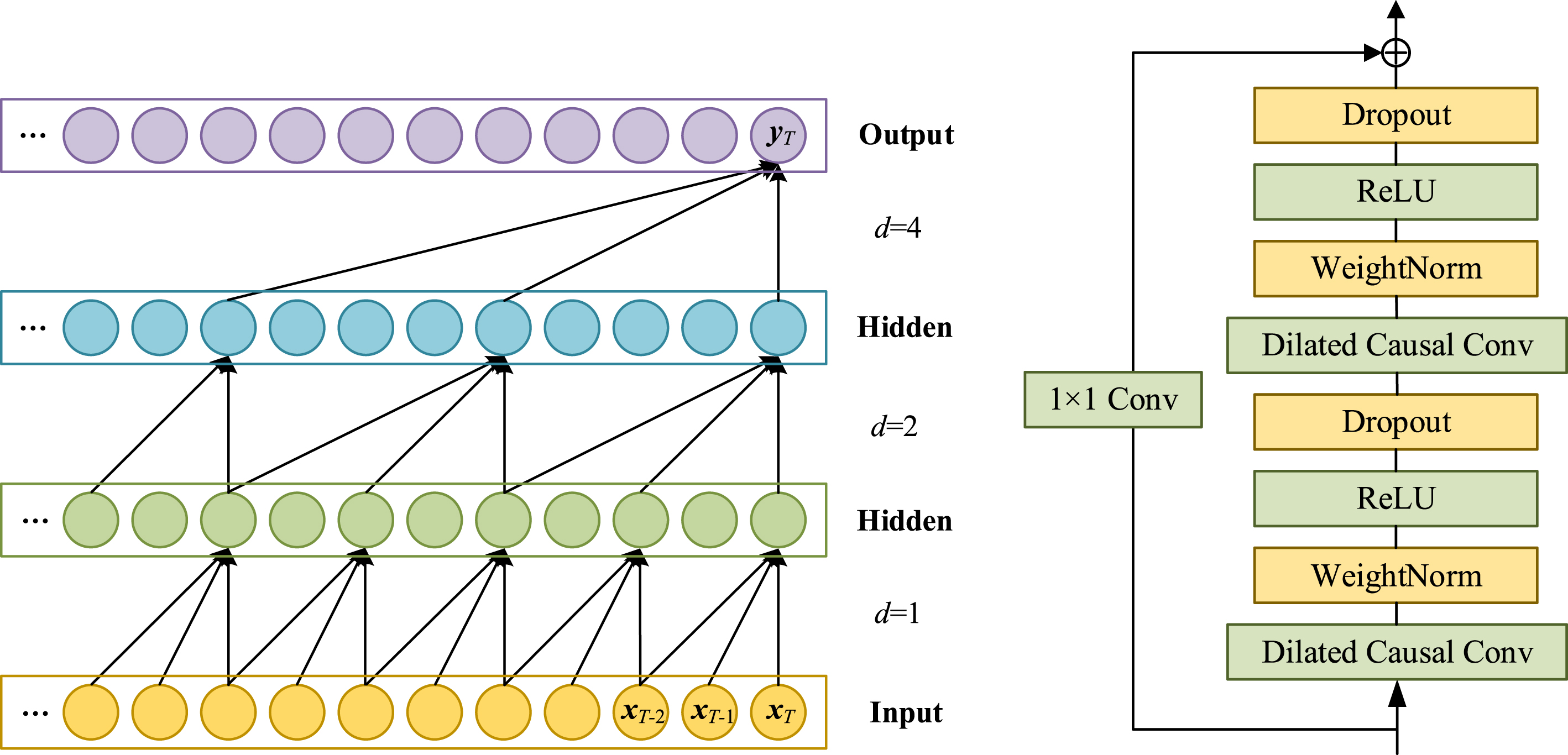
(a) The structure of the dilated causal convolution. (b) The structure of the TCN module.

As shown in Fig. 2 (a), the input layer sampling rate is d = 1, which represents that each input data is sampled in 1D (one-dimensional) convolution and fed into the next layer. The sampling rate of the first hidden layer, d = 2, represents that one sample is taken as input every 2 samples, and so on; as the layers deepen, the causal dilated convolution makes the size of the receptive field grow exponentially during the convolution operation, effectively acquiring a larger receptive field and capturing longer temporal information. The causal convolution structure ensures that the current output value depends only on the current and past data, i.e., the output y_T at time T is only relevant to x₁, x₂, …, x_T, preventing future data from being leaked during the prediction.

The size of the receptive field in the TCN module has a strong relationship to the number of network layers, and if the network is designed too deep in order to expand the receptive field, the existence of the dilated causal convolution will inevitably lead to a more complex network structure and reduced efficiency and stability, which can easily cause gradient disappearance and gradient explosion [28]. Therefore, the TCN module introduces residual connections, which alleviate the gradient disappearance [22] and effectively improve the performance. The overall network structure is shown in Fig. 2 (b).

3.5 Graph attention network component

The GAT belongs to one of the GNN models, which can better capture the correlations between different types of nodes than the traditional attention mechanisms.

The GAT layer can model the relationship between any two graph nodes. Let a graph have k nodes, denoted as {v₁, v₂, …, v_k}. v_i is the input vector of the node i, whose output vector h_i is calculated as: $h_{i} = σ (\sum_{j = 1}^{L} α_{ij} v_{j})$ (2) where h_i has dimension consistent with that of v_i, and is used to replace the original vector v_i as the output of the GAT layer; σ represents the sigmoid activation function; α_ij is the attention weight of node j for node i; and L is the total number of nodes neighboring node i. The attention weights α_ij can be calculated by the following equations. $e_{ij} = LeakyReLU (w^{T} \cdot (v_{i} \oplus v_{j}))$ (3) $α_{ij} = \frac{exp (e_{ij})}{\sum_{l = 1}^{L} exp (e_{ij})}$ (4)

Here, ⊕ denotes two vectors concatenate with each other, LeakyReLU is a nonlinear activation function [4] and w is a learnable weight parameter. This paper follows the literature [15] for the design, which uses a feature-based graph attention layer and a time-based graph attention layer in parallel.

Feature-based graph attention layer: A set of multivariate time series data is considered as a graph, where the time series data of each feature is represented by a node, and the relationship between two corresponding features is represented as an edge between two nodes. This allows modeling the relationship between adjacent nodes using graph attention, where T is the number of timestamps and k is the number of features. We take the number of nodes as 6 as an example, and the structure is schematically shown in Fig. 3.

Time-based graph attention layer: This layer uses the GAT to capture the temporal correlation in time series. Each node represents the vector at the moment of timestamp t, and its neighboring nodes are all other timestamps within the current sliding window. Just as feature-based GAT notices similarity between vectors corresponding to two feature nodes, time-based GAT notices similarity between vectors every two moments. The output of the time-oriented graph attention layer is also a k×T matrix.

Fig. 3

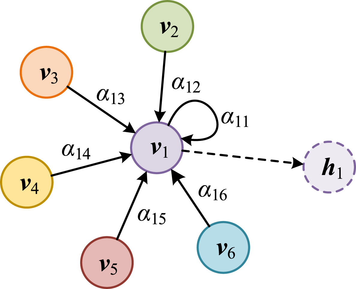
The structure of the feature-based GAT component. The dashed circle is the final output.

3.6 GRU-attention component

After concatenating the output of the two GAT layers with the output of the sample TCN module, we obtained a matrix of 3k×T and fed it into the GRU-Attention component. The component comprises a GRU followed by a layer of attention mechanisms based on the Gaussian kernel.

As an improved model of LSTM, the GRU model reduces the internal design of a door to simplify the model structure and better capture long-term time-series information to mitigate gradient disappearance in LSTM models.

The outputs of the GRU layer are fed into the temporal-Gaussian kernel attention mechanism, as shown in Fig. 4. The significant advantage of the attention mechanism is that it focuses on the relevant information and ignores the irrelevant information. The attention mechanism is calculated to increase the weight of critical information and decrease the weight of non-critical information. Therefore, it well models sequence data with variable length, and also has a strong ability to capture long-term dependent information, which can effectively improve the accuracy of temporal sequence modeling.

Fig. 4

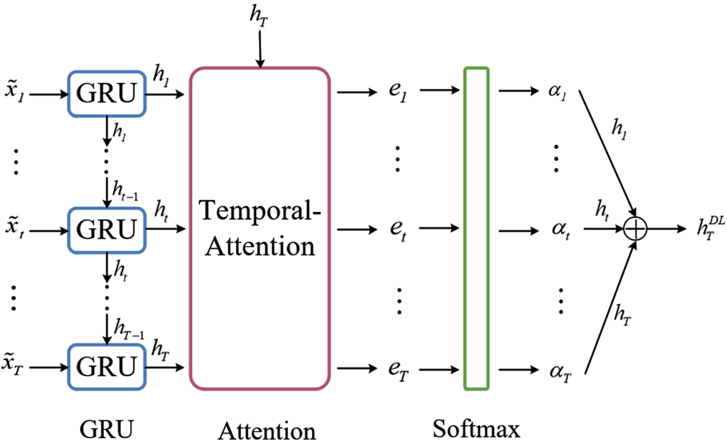
The structure of the GRU-Attention component.

In classical attention mechanism, similarity is generally measured by the inner product kernel function. Since the Gaussian kernel function is the more effective and stable, this paper introduces the Gaussian kernel function into the attention mechanism. It is also possible to combine multiple kernel functions to create a more suitable similarity measure formula. To reduce the operations of the model, only one kernel function of the Gaussian kernel is used in this paper, and taking the Fig. 4 as an example, the formula for measuring the similarity e_t (h_t, h_T) between two vectors h_t and h_T is as follows. $e_{t} (h_{t}, h_{T}) = exp (- \frac{{∥ h_{t} - h_{T} ∥}^{2}}{2 σ^{2}})$ (5)

The above t is taken as 1, …, T, h_t is the output of the GRU at time t, and then the e₁, …, e_T is input into the softmax layer as seen in Fig. 4, so we get the attention weights α₁, …, α_T. Specifically, the attention weight α_t is used to denote the similarity of the hidden layer state h_T at the ultimate moment T to the h_t at the moment t. It represents the importance of the hidden layer state at each timestamp to the output state at the ultimate moment. Finally, the GRU-Attention layer represents the output vector as a weighted sum of the hidden layer states at all times. $h_{T}^{DL} = \sum_{t = 1}^{T} α_{t} h_{t}$ (6)

3.7 Auto-regressive component

Due to the nonlinear nature of the convolution component, the graph attention component and the recurrent component, the neural network model may be complex and unstable. To reduce the model complexity and enhance its robustness, this paper follows the study in the literature [13] and decomposes the final prediction of the model into the sum of the linear component, which focuses on the overall trend, and the neural network component, which focuses on specific fluctuations. We use the classical AR model as the linear component, which is computed as: $y_{T + 1, i}^{AR} = \sum_{t = 1}^{T} W_{t}^{AR} x_{t, i} + b^{AR}$ (7)

The output prediction of the AR module is denoted as $y_{T + 1}^{AR} \in R^{k}$ , which spliced by the $y_{T + 1, i}^{AR}$ under each feature, where $W_{t}^{AR}$ is the weight matrix of the AR model. We implement this model using a dense layer of network to combine the weights and data.

3.8 Joint optimization

Since the prediction model and the reconstruction model have their respective advantages, we combine the two models in the same way as MTAD-GAT. The resultant model consists of a prediction-based model to predict the value of the next timestamp and a reconstruction-based model to reconstruct the data distribution of the whole time series. In the training process, the parameters of two modules are updated simultaneously and jointly optimized. We have made some robustness improvements and module simplifications for the prediction module and the reconstruction module, respectively.

In the prediction model, we first feed the output $h_{T}^{DL}$ of the GRU-Attention layer into a fully connected layer to obtain the prediction $y_{T + 1}^{DL} \in R^{k}$ of the neural network layer, and then add it to the prediction of the parallel AR module to obtain the total prediction value, which is calculated as follows. ${\hat{y}}_{T + 1} = y_{T + 1}^{DL} + y_{T + 1}^{AR}$ (8)Loss_pre denotes the loss function of the prediction model, and the loss function uses the root mean square, illustrated in Equation (9). $Los s_{pre} = \sqrt{\sum_{i = 1}^{k} {({\hat{y}}_{t, i} - y_{t, i})}^{2}}$ (9)

In the reconstruction model, unlike the MTAD-GAT model that used a Variational Auto-Encoder (VAE) [10], the RNN decoder is used to reconstruct the output of the GRU-Attention layer to simplify the module. We decode the implied vector $h_{T}^{DL}$ of GRU-Attention output using RNN decoder to obtain the reconstructed output vector ${\hat{x}}_{1}, \dots, {\hat{x}}_{T}$ of the original input x₁, …, x_T. Loss_rec denotes the loss function of the reconstruction model, illustrated in Equation (10). ${Loss}_{rec} = \sqrt{\sum_{t = 1}^{T} {({\hat{x}}_{t} - x_{t})}^{2}}$ (10)

The total loss function of the model is defined as the sum of the above two loss functions, i.e. $Loss = {Loss}_{pre} + {Loss}_{rec}$ (11)

3.9 Threshold selection

We also use Peak Over Threshold (POT) [3 , 28] to choose the threshold automatically. Specifically, the anomaly score at time T + 1 can be calculated by Equation (12). $s_{T + 1} = \frac{\sum_{i = 1}^{k} {({\hat{y}}_{T + 1, i} - y_{T + 1, i})}^{2} + c \times \sum_{t = 1}^{T} {({\hat{x}}_{t} - x_{t})}^{2}}{1 + c}$ (12)

For the time T + 1, the anomaly score is a linear combination of the prediction error at time T + 1 and the reconstruction error at times 1 to t; the coefficient c is used to balance the prediction-based error and the reconstruction-based error; k is the number of features. The anomaly score at each moment in the testing set is denoted as {s₁, s₂, …, s_Q} ∈ R^Q, where Q is the number of samples in the testing set.

The anomaly score is calculated for each timestamp, and if the anomaly score at time t is greater than the threshold, it is treated as an anomaly.

4 Experiments

4.1 Datasets

In this section, we illustrate the performance of the proposed model on three datasets including MSL, SMAP, and SMD. The first two, MSL and SMAP [29], are spacecraft public datasets from NASA, collected by the Mars Science Laboratory rover ‘Curiosity’ and Soil Moisture Active Passive Satellite, respectively, with anomalies flagged by experts. The SMD dataset [35] consists of five weeks of data from a company’s server.

The statistics of these three datasets are presented in Table 1.

Table 1
Dataset information

Dataset MSL SMAP SMD

Number of attributes 55 25 38

Training set size 58317 135183 708425

Testing set size 73729 427617 708420

Anomaly rate (%) 10.72 13.13 4.16

Dataset	MSL	SMAP	SMD
Number of attributes	55	25	38
Training set size	58317	135183	708425
Testing set size	73729	427617	708420
Anomaly rate (%)	10.72	13.13	4.16

4.2 Metrics and parameters

In this paper, Precision, Recall and F1 score are used to compare and evaluate the performance of MTAD-TCGA algorithm with other algorithms. The larger the values of the three indicators, the more desirable the model is. As with most methods, we used the point-adjust method [35] to measure performance. If the algorithm can detect any point in the anomaly region, we consider all points in the region to be correctly detected.

Some parameters of the model are set as follows: the sliding window T is taken as 100, the sampling rate d in the TCN module is taken as [1 , 8], the dimensionality of the GRU hidden layer is 200; the POT threshold q is selected with 0.001. We use the Adam optimizer for stochastic gradient descent for 40 epochs with an initial learning rate 0.001 during model training. All experiments in this study are conducted on NVIDIA GeForce GTX 3090 GPU.

4.3 Comparison with baselines

We compared the model of this paper with four other advanced models on three public datasets, including LSTM-NDT [23], DAGMM [5], Omni-Anomaly [35], and MTAD-GAT [15]. The comparative results of the metrics are shown in Table 2, and F1 scores for each model are shown in Fig. 5.

Table 2
Performance of MTAD-TCGA and four baseline approaches

Methods MSL SMAP SMD

Precision Recall F1 Precision Recall F1 Precision Recall F1

LSTM-NDT 0.5934 0.5374 0.564 0.8965 0.8846 0.8905 0.5684 0.6438 0.6037

DAGMM 0.5412 0.9934 0.7007 0.5845 0.9058 0.7105 0.5951 0.8782 0.7094

OmniAnomaly 0.8867 0.9117 0.8989 0.7416 0.9776 0.8434 0.8334 0.9449 0.8857

MTAD-GAT 0.8906 0.9123 0.9013 0.8754 0.9440 0.9084 0.9409 0.8524 0.8945

MTAD-TCGA 0.8530 0.9852 0.9144 0.9261 0.9283 0.9272 0.8709 0.9751 0.9201

Methods	MSL	SMAP	SMD
LSTM-NDT	0.5934	0.5374	0.564	0.8965	0.8846	0.8905	0.5684	0.6438	0.6037
DAGMM	0.5412	0.9934	0.7007	0.5845	0.9058	0.7105	0.5951	0.8782	0.7094
OmniAnomaly	0.8867	0.9117	0.8989	0.7416	0.9776	0.8434	0.8334	0.9449	0.8857
MTAD-GAT	0.8906	0.9123	0.9013	0.8754	0.9440	0.9084	0.9409	0.8524	0.8945
MTAD-TCGA	0.8530	0.9852	0.9144	0.9261	0.9283	0.9272	0.8709	0.9751	0.9201

Fig. 5

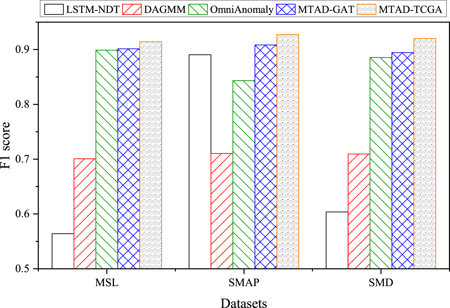
F1 scores of MTAD-TCGA and all baseline models.

By comparing these F1 scores of different models reported in Table 2, we find that MTAD-TCGA performs consistently and excellently, achieving the highest F1 score on all datasets, with no extreme values for Precision and Recall values, proving that our model has good accuracy and generalization ability. LSTM-NDT only has a high score on SMAP, indicating that the model may be sensitive to different types of datasets. The shortcoming of the DAGMM model is that it does not consider temporal time series information well, while the two time-based attentions designed in the model of this paper can effectively help capture the temporal dependencies of time series data. OmniAnomaly and MTAD-GAT, as one of the most advanced models at present, can perform well on all three datasets, but this in paper multiple modules are de signed with a more comprehensive consideration, which makes the models in this paper superior to those models on all three datasets.

Visualizing the effect of the models in this paper allows finding anomalies for further analysis of the model results. First, we take the 2-3 server in the SMD dataset as an example and plot the anomaly scores, predicted anomalies, and the actual anomalies for each moment in the testing set, and we selected part of the testing set data from the 1-6 server in the SMD dataset and plotted the anomaly scores with the thresholds. The two visualizations are shown in Figs. 6 7.

Fig. 6

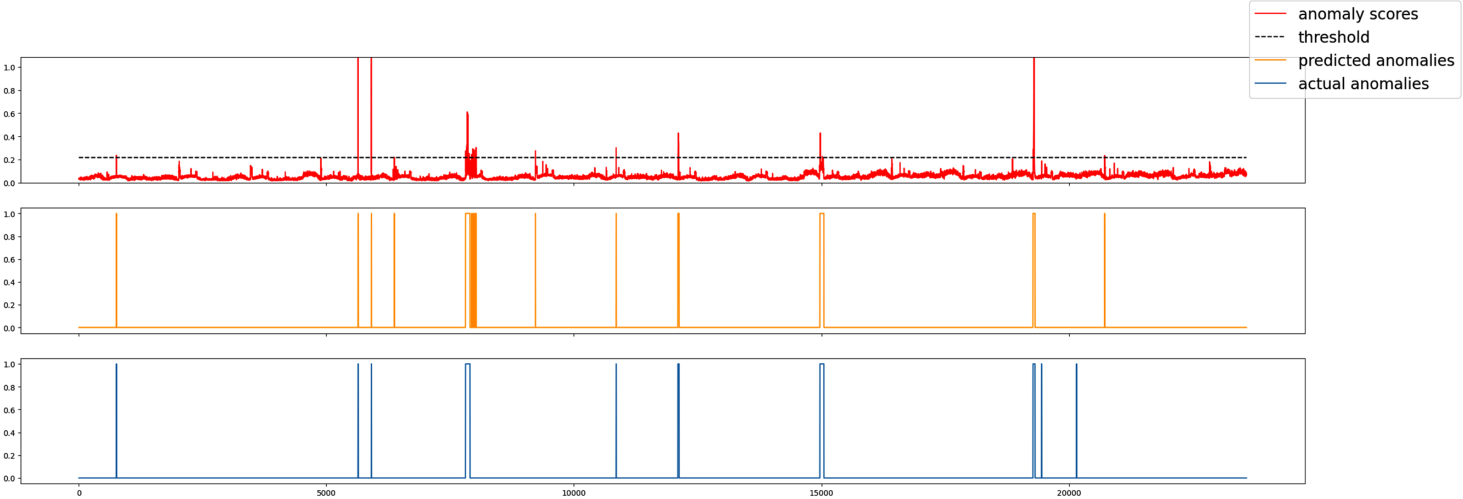
Comparison of anomaly scores, predicted anomalies, and actual anomalies (SMD).

Fig. 7

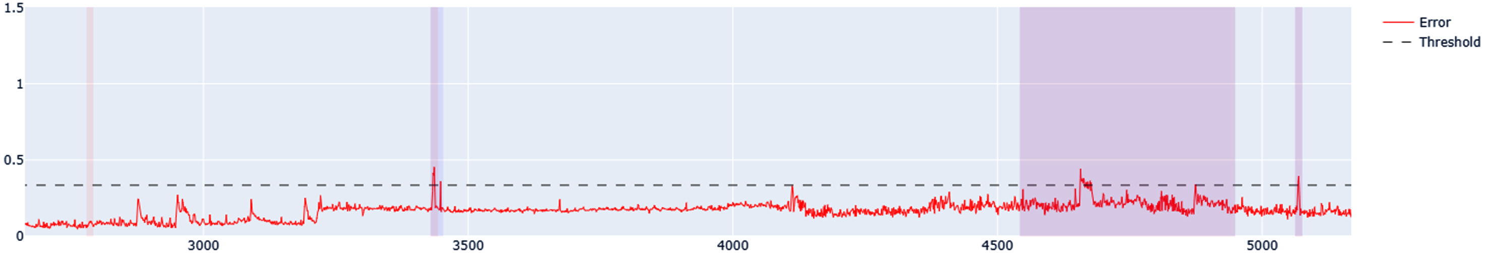
The effect of anomaly detection on the SMD dataset for some testing sets.

Comparing the three sections of Fig. 6 shows that the predicted anomalies of this paper’s model differ little from the actual anomalies, and it can clearly show which timestamps are anomaly moments. For Fig. 7, where the blue and red area indicate wrongly detected samples. The blue area denotes samples predicted to be anomalies but normal samples in fact and the red area denotes samples which predicted to be normal samples but anormal samples in fact. The purple area indicates correctly detected samples, i.e., samples predicted to be anomalies and also anomalies in fact, it can be seen that the model has a high accuracy in the prediction of anomalies. The effectiveness of the MTAD-TCGA model is visually con-firmed in Figs. 6 7.

4.4 Ablation study

In order to discuss the model components more completely and to clarify the necessity and validity of inclusion of each component used to improve performance, three sets of ablation experiments were designed, each changing a component. The experiments were conducted after using the TCN component, the Attention component, and the AR component from the original MTAD-GAT model. F1 scores were obtained from each experiment; the results are shown in Table 3.

Table 3
F1 scores in ablation study

Methods MSL SMAP SMD

MTAD-GAT 0.9013 0.9084 0.8945

+TCN 0.9096 0.9238 0.9144

+Attention 0.9080 0.9111 0.9121

+AR 0.9058 0.9096 0.9023

Methods	MSL	SMAP	SMD
MTAD-GAT	0.9013	0.9084	0.8945
+TCN	0.9096	0.9238	0.9144
+Attention	0.9080	0.9111	0.9121
+AR	0.9058	0.9096	0.9023

Table 3 shows that the several components have different effects on the results from the test datasets. Adding the AR layer has the least impact on the improvement of the overall model accuracy, which could be expected, because the AR layer is introduced mainly to enhance model stability. The TCN and Gaussian-Attention layers are involved in modeling the temporal dimension, and they all increase the F1 score. The ablation experiments show that each component added to the original model is individually effective in improving the modeling long time series relations contributing to the combined improvements re-ported in Table 2.

5 Conclusion

We improve on the MTAD-GAT framework and present a novel algorithmic framework, MTAD-TCGA, for anomaly detection on multivariate time series data. The model captures long-term time series dependencies more effectively by combining TCN, GAT, and GRU-Attention modules. Extensive experiments on public datasets from spacecraft and server show that the accuracy of our proposed algorithm outperforms other advanced methods. The direction of future work in seeking further improvement could involve two aspects: first, reducing the time and space complexity of the model while improving its accuracy, and second, enhancing the anomaly diagnosis capability and interpretability of the model.

Footnotes

Acknowledgments

This work is supported by National Natural Science Foundation of China (Nos. 62072024), R&D Program of Beijing Municipal Education Commission (KM202110016001, KM202210016002), Scientific Research Foundation of Beijing University of Civil Engineering and Architecture (Nos. KYJJ2017017 and Y19-19), Projects of Beijing Advanced Innovation Center for Future Urban Design, Beijing University of Civil Engineering and Architecture (Nos. UDC2019033324).

References

Deng

and Hooi

, Graph Neural Network-Based Anomaly Detection in Multivariate Time Series (2021).

Bianco

A.M.

, Martinez

E.J.

, Garcia Ben

and Yohai

V.J.

, Robust procedures for regression models with ARIMA errors, Physica-Verlag HD (1996).

Siffer

, Fouque

P.A.

, Termier

and Largouet

, Anomaly Detection in Streams with ExtremeValue Theory// Acm Sigkdd International Conference. ACM (2017).

, Wang

N.Y.

, Chen

T.Q.

and Li

, Empirical evaluation of rectified activations in convolutional network, Computer Science (2015).

Zong

, Song

, Min

M.R

, et al., Deep autoencoding gaussian mixture model for unsupervised anomaly detection// International Conference on Learning Representations (2018), 781–795.

Szegedy

, Liu

, Jia

, et al., Going deeper with convolutions, IEEE Computer Society (2014).

Hawkins

D.M.

, Identification of outliers, Biometrics 37(4) (1981), 860.

Park

, Hoshi

and Kemp

C.C.

, A multimodal anomaly detector for robot-assisted feeding using an LSTM-based variational autoencoder, IEEE Robotics and Automation Letters 3 (2018), 1544–1551.

Kingma

D.P.

and Welling

, Auto-Encoding Variational Bayes (2014).

10.

Kingma

D.P.

and Welling

, An Introduction toVariational Autoencoders (2019).

11.

Shafeiy

E.A.

, Desouky

A.I.

and Eghamrawy

S.M.

, Prediction of liver diseases based on machine learning technique for big data, International Conference on Advanced Machine Learning Technologies and Applications. Springer (2018), 362–374.

12.

Box

G.E.P.

and Jenkins

G.M.

, Time series analysis: forecasting and control, Journal of Time 31(3) (2010).

13.

Lai

, Chang

W.C.

, Yang

and Liu

, Modeling long and short-term temporal patterns with deep neural networks, ACM (2018).

14.

Ren

, Xu

, Wang

, et al., Time-Series Anomaly Detection Service at Microsoft// Acm Sigkdd International Conference. ACM (2019).

15.

Zhao

, Wang

, Duan

, Huang

and Zhang

, Multivariate Time-series Anomaly Detection via Graph Attention Network (2020).

16.

Audibert

, et al., USAD: UnSupervised Anomaly Detection on Multivariate Time, KDD (2020).

17.

Chen

, Yin

, Li

, Yang

and Hong

, One-dimensional convolutional neural network based bearing fault diagnosis, Open Access Library Journal 9(4) (2022), 11.

18.

Chung

, Gulcehre

, Cho

and Bengio

, Empirical evaluation of gated recurrent neural networks on sequence modeling (2014).

19.

Chou

J.S.

and Telaga

A.S.

, Real-time detection of anomalous power consumption, Renewable & Sustainable Energy Reviews 33(5) (2014), 400–411.

20.

Connor

J.T.

, Atlas

L.E.

and Martin

R.D.

, Recurrent networks and NARMA modelling, Advances in Neural Information Processing Systems (1992), 01–308.

21.

, Wu

, et al., Anomaly Transformer: Time Series Anomaly Detection with Association Discrepancy, ICLR (2022).

22.

, Zhang

, Ren

and Sun

, Deep Residual Learning for Image Recognition// 2016 IEEE Conference on ComputerVision and Pattern Recognition (CVPR). IEEE (2016).

23.

Hundman

, Constantinou

, Laporte

, Colwell

and Soderstrom

, Detecting Spacecraft Anomalies UsingLSTMs and Nonparametric Dynamic Thresholding (2018).

24.

Quan

and Zhou

, Research on multivariate time series data anomaly detection method based on KPCA[J], Computer Measurement and Control 19(4) (2011), 822–825.

25.

Defferrard

, Bresson

and Vandergheynst

, Convolutional neural networks on graphs with fast localized spectral filtering, Advances in Neural Information Processing Systems 3844–3852.

26.

Gupta

, Gao

, Aggarwal

C.C.

and Han

, Outlier detection for temporal data: a survey, IEEE Transactions on Knowledge & Data Engineering 26(9) (2014), 2250–2267.

27.

Breunig

M.M.

, Kriegel

H.P.

, Ng

R.T.

and Sander

, LOF: identifying density-based local outliers. Proceedings of the 2000 ACMSIGMOD international conference on Management of data (2000), 93–104.

28.

Hewage

, Behera

, Trovati

, Pereira

and Liu

, Temporal convolutional neural (TCN) network for an effective weather forecasting using time-series data from the local weather station, Soft Computing 24(21) (2020).

29.

O’Neill

, Entekhabi

, Njoku

and Kellogg

, The NASA Soil Moisture Active Passive (SMAP) mission: Overview// Geoscience & Remote Sensing Symposium. IEEE (2010).

30.

Velikovi

, Cucurull

, Casanova

, et al. Graph Attention Networks// 2017.

31.

Bai

, Kolter

J.Z.

and Koltun

, An Empirical Evaluation of Generic Convolutional and Recurrent Networks for Sequence Modeling (2018).

32.

Hochreiter

and Schmidhuber

, Long short-term memory, Neural Computation 9(8) (1997), 1735–1780.

33.

Kipf

T.N.

and Welling

, Semi-supervised classification with graph convolutional networks (2016).

34.

Chen

X.H.

, et al., DAEMON: Unsupervised Anomaly Detection and Interpretation for Multivariate Time Series, the 37th International Conference on Data Engineering, IEEE (2021).

35.

, Zhao

, Niu

, Liu

and Pei

, Robust Anomaly Detection for Multivariate Time Series through Stochastic Recurrent Neural Network// the 25th ACM SIGKDD International Conference. ACM (2019).

36.

Z.H.

, et al., Connecting the Dots: Multivariate Time Series Forecasting with Graph Neural Networks, KDD (2020).

Methods	MSL			SMAP			SMD
	Precision	Recall	F1	Precision	Recall	F1	Precision	Recall	F1
LSTM-NDT	0.5934	0.5374	0.564	0.8965	0.8846	0.8905	0.5684	0.6438	0.6037
DAGMM	0.5412	0.9934	0.7007	0.5845	0.9058	0.7105	0.5951	0.8782	0.7094
OmniAnomaly	0.8867	0.9117	0.8989	0.7416	0.9776	0.8434	0.8334	0.9449	0.8857
MTAD-GAT	0.8906	0.9123	0.9013	0.8754	0.9440	0.9084	0.9409	0.8524	0.8945
MTAD-TCGA	0.8530	0.9852	0.9144	0.9261	0.9283	0.9272	0.8709	0.9751	0.9201

Multivariate time-series anomaly detection via temporal convolutional and graph attention networks

Abstract

Keywords

1 Introduction

2 Related work

3 Proposed framework

3.1 Problem statement

3.2 Overview

4.1 Datasets

Table 1 Dataset information Dataset MSL SMAP SMD Number of attributes 55 25 38 Training set size 58317 135183 708425 Testing set size 73729 427617 708420 Anomaly rate (%) 10.72 13.13 4.16

4.3 Comparison with baselines

Table 3 F1 scores in ablation study Methods MSL SMAP SMD MTAD-GAT 0.9013 0.9084 0.8945 +TCN 0.9096 0.9238 0.9144 +Attention 0.9080 0.9111 0.9121 +AR 0.9058 0.9096 0.9023

Footnotes

Acknowledgments

References

Table 1
Dataset information

Dataset MSL SMAP SMD

Number of attributes 55 25 38

Training set size 58317 135183 708425

Testing set size 73729 427617 708420

Anomaly rate (%) 10.72 13.13 4.16

Table 3
F1 scores in ablation study

Methods MSL SMAP SMD

MTAD-GAT 0.9013 0.9084 0.8945

+TCN 0.9096 0.9238 0.9144

+Attention 0.9080 0.9111 0.9121

+AR 0.9058 0.9096 0.9023