A hybrid method of time series forecasting based on information granulation and dynamic selection strategy 1

Abstract

Forecasting trend and variation ranges for time series has been challenging but crucial in real-world modeling. This study designs a hybrid time series forecasting (FIGDS) model based on granular computing and dynamic selection strategy. Firstly, with the guidance of the principle of justifiable granularity, a collection of interval-based information granules is formed to characterize variation ranges for time series on a specific time domain. After that, the original time series is transformed into granular time series, contributing to dealing with time series at a higher level of abstraction. Secondly, the L₁ trend filtering method is applied to extract trend series and residual series. Furthermore, this study develops hybrid predictors of the trend series and residual series for forecasting the variation range of time series. The ARIMA model is utilized in the forecasting task of the residual series. The dynamic selection strategy is employed to identify the ideal forecasting models from the pre-trained multiple predictor system for forecasting the test pattern of the trend series. Eventually, the empirical experiments are carried out on ten time series datasets with a detailed comparison for validating the effectiveness and practicability of the established hybrid time series forecasting method.

Keywords

Granular computing information granule time series forecasting dynamic selection

1 Introduction

Time series data is a series of data points collected by their occurrence in time, which emerges in various areas, including economy [1], health care [2], energy management [3], hydrology [4], and electric power system [5], etc. Therefore, developing an ideal forecasting method is a crucial task in time-series modeling, which is a prerequisite for scientific decision-making. However, due to the characteristics of time series data presenting different patterns over time, selecting the most suitable forecasting models is a highly challenging task.

A large number of time series forecasting theories and methods have been proposed from different perspectives, including classical statistical models and machine learning algorithms.

The autoregressive (AR) model [6] and autoregressive moving average (ARMA) model [7] are well-known classical statistical models for stationary time series. By incorporating an initial differencing step in the ARMA model, the autoregressive integrated moving average (ARIMA) model [8] can work well on the time series with non-stationarity. Holt-Winters exponential smoothing [9] forecasts new samples by calculating the weighted average of the current value and the previous smoothed observation, which effectively deal with non-stationary series. To solve the problems with non-constant variance of the volatility of the time series, the non-linear autoregressive conditional heteroskedasticity (ARCH) model [10] and the generalized autoregressive conditional heteroskedasticity (GARCH) model [11] have been developed for characterizing the fluctuation levels. These classical models have been developed based on specific assumptions on trends or error distributions. Without relying too much on assumptions, machine learning models, including artificial neural networks (ANN) [12], support vector regression (SVR) [13], harmonic regression [14], and long short-term memory (LSTM) [15], offer promising alternatives to analyze the non-direct relationships hidden in time series. However, although these methods have been practical in diverse fields, no one forecasting algorithm performs well for all cases according to the no-free-lunch theorem [16]. Many scholars have attempted to construct various time series forecasting models to avoid a single model that may generate unsatisfactory results by incorporating an ensemble learning strategy.

The ensemble method has been acknowledged as a promising way of improving forecasting systems’ robustness. Li et al. [17] proposed a heterogeneous ensemble forecasting model with multi-objective programming for nonlinear time series, verifying that the forecasting performance is better than the individual models. Du et al [18] employed a Bayesian optimization-based dynamic ensemble method, overcoming the limitation of a single forecasting model.

Dynamic selection offers a strategy to identify the elite model from the multiple predictors to forecast each test pattern [16]. The merit of the dynamic selection makes multiple predictor system (MPS) not depend on the same models but dynamically select the ideal models for each new pattern according to the nature and behavior of the time series. The multiple predictor system (MPS) incorporating dynamic selection has exhibited better superiority and forecasting precision. However, the inputs and outputs of most forecasting methods are numerical values, and the variation ranges for future time series are not depicted enough. Therefore, the forecasting models with ideal variation ranges and accuracies are pursing in modeling time series.

Granular computing (GrC) [19] offers a novel way for data process and information interpretation based on simulating the human problem-solving mechanism. Information granule [20], as a base unit of granular computing, can hold the internal characteristics and critical information, on which some granular models have been developed for effectively solving problems at an abstract level. The principle of justifiable granularity [21] is a key guideline for constructing and optimizing information granules, involving two conflicting requirements: coverage and sound semantic. The principle of justifiable granularity has been employed to transform the original time series into the corresponding granular versions, efficiently capturing the primary information of the original time series. The time series forecasting models based on the principle of justifiable granularity [22, 23], exhibit competitive advantages in dimension reduction and long-term prediction. By incorporating information granulation into time series forecasting, the outputs are information granules, which can be used in characterizing variation ranges of the future time series.

This study is to develop a hybrid time series forecasting (FIGDS) model based on information granulation and dynamic selection strategy, aiming to offer variation ranges and sound forecasting performance. The developed method first obtains the interval granular time series for obtaining the variation ranges in the specific period. Second, we obtain the trend series and residual series by using L₁ trend filtering technique. In the prediction process, the dynamic selection strategy is employed to identify the predictor from the pre-trained multiple predictors for trend series forecasting, and the ARIMA model is utilized for forecasting residual series. Finally, the forecasting results on the trend series and residual series are integrated to form interval information granules. The contributions of the designed method can be summarized as follows:

The granular time series inherits the main essence of the original time series and characterizes the variation ranges in the specific period.

The information granules generated from the trend and residual series forecasting effectively describe the trends and the variation ranges of future time series.

The forecasting model incorporating a dynamic selection strategy exhibits sound forecasting accuracy in prediction.

The remaining parts of this study are structured as follows: Section 2 formulates the theoretical foundation for the designed hybrid model. Section3 details the procedure of the FIGDS model. The performance metrics are presented in Section 4 Section 5 focuses on carrying on experiment verification and exhibiting empirical results on ten datasets compared with other approaches. Finally, the conclusion is presented in Section 6.

2 Theoretical foundation

This section offers the theoretical foundation of the proposed hybrid time series forecasting model.

2.1 Time series granulation

Following the principle of justifiable granularity, the numeric time series can be transformed into the sequence of information granules in chronological order, through which the dimensionality is reduced. In what follows, let us firstly focus on how to realize the granulation of the time series.

Given a numeric time series x₁, x₂, ⋯ , x_n, the granulation is realized by dividing the time domain T = {1, 2, ⋯ , n} into k non-overlapping time intervals T₁, T₂, ⋯ , T_k. Therefore, the whole time series can be expressed as k non-overlapping sequences s₁, s₂, ⋯ , s_k. For i-th sequence s_i, an optimal interval-based information granule Ω_i = [a_i, b_i] is constructed by employing the principle of justifiable granularity [21]. In this process, two sound and intuitively appealing criteria, namely: coverage and sound semantics, are taken into account. The first one requires the information granule Ω_i to cover the data points as much as possible in the sequence s_i, which makes the information granule Ω_i more experimentally and serves as a reasonable quantification. In general, an increasing function f₁ of the cardinality card {x_j|x_j ∈ Ω_i} is employed to describe the role of coverage. The second criterion requires that the information granule constructed is as specific as possible, which can be characterized by a decreasing function f₂ of the length of interval m(Ω_i) = |b_i - a_i|. A smaller value of f₂ means well-articulated semantics. Keeping these two conflicting requirements into account, it is a reasonable way to consider the product of these functions: f = f₁ · f₂. The following way is considered to form the interval-based information granule [24]: $f_{1} = card {x_{j} | x_{j} \in Ω_{i}},$ (1) $f_{2} = 1 - \frac{m (Ω_{i})}{\max (s_{i}) - \min (s_{i})},$ (2) where max(s_i) and min(s_i) represent the maximum and minimum value of the sequence s_i, respectively.

The process to construct the interval-based information granule Ω_i is firstly realized by seeking the representative element rep (s_i), the optimal lower bound a_i, and optimal upper bound b_i. Since the average is a crucial measure to describe the central level of data, the average of the sequence s_i is experimentally regarded as the representative point, denoted as rep (s_i). Nextly, the optimal lower bound a_i and optimal upper bound b_i of the information granule Ω_i can be determined by applying the function f on the left part $Ω_{i}^{-} = [a_{i}, rep (s_{i})]$ and right part $Ω_{i}^{+} = [rep (s_{i}), b_{i}]$ of the representative element rep (s_i), independently. That is $a_{i, opt} = \max_{a_{i} \leq rep (s_{i})} (V (a_{i})),$ (3) $b_{i, opt} = \max_{rep (s_{i}) \leq b_{i}} (V (b_{i})),$ (4) and $V (a_{i}) = f_{1} (Ω_{i}^{-}) f_{2} (Ω_{i}^{-})$ , $V (b_{i}) = f_{1} (Ω_{i}^{+}) f_{2} (Ω_{i}^{+})$ .

Through the process mentioned above, each sequence s_i can be granulated into an interval-based information granule Ω_i = [a_i, b_i]. The information granulation of time series not only offers a way to represent and deal with time series at a higher abstract level for capturing its main essence but also provides a concise description for the original time series [24].

2.2 L₁ trend filtering

Since trend information is a critical feature in time series, developing a forecasting model considering trend information has attracted much attention. L₁ trend filtering [25], as an extension on Hodrick-Prescott (H-P) filtering [26], is an important method to analyze the primary linear trend of time series, which is an efficient algorithm for estimating the potential trend in time series. It is also an approximation way of the original time series with line segment representation. L₁ trend filtering gets plenty of potential applications in time series forecasting fields. For example, L₁ trend filtering is applied to produce an optimal segmentation of time series for time series clustering [27].

For the original time series x = {x₁, x₂, ⋯ , x_t}, the role of L₁ trend filtering is to extract a smooth trend series y_t existing in time series x and obtain a residual series z_t (t = 1, 2, ⋯ , n) which is as small as possible. L₁ trend filtering can be realized by minimizing the following optimization problem: $\begin{matrix} Min Q (x) = (1 / 2) \sum_{t = 1}^{n} (x_{t} - y_{t})^{2} + \\ λ \sum_{t = 2}^{n - 1} | y_{t - 1} - 2 y_{t} + y_{t + 1} |, \end{matrix}$ (5) which also can be written in the forming of the matrix as follows: $Min Q (x) = | | x - y | |_{2}^{2} + λ | | D x | |_{1},$ (6) where ||u||₁ = ∑_i|u_i|, ||u||₂ = (∑_i|u_i|²) ^1/2, λ is a nonnegative weighted parameter for balancing the smooth trend and the size of the residual time series. D ∈R^(n-2)×n is the second-order difference matrix.

2.3 Autoregressive integrated moving average (ARIMA)

The autoregressive integrated moving average (ARIMA) [8] model, as a representative of the econometric model, is one of the classical statistical time series analysis techniques, which has been widely applied for non-stationary time series data analysis in the reference literature. Driven by the Box-Jenkins model [28] (1960), ARIMA model is built to make full use of the past value to predict the future values of time series, which can be described as a linear combination of autoregressive (AR) and moving average (MA) components. The ARIMA model consists of three stages: model identification, parameter estimation, and diagnostic check, through which an adaptive and optimal forecasting model is determined. The ARIMA(p,d,q) model can be expressed as follows. $\begin{matrix} x_{t} = c + Φ_{1} x_{t - 1} + \dots + Φ_{p} x_{t - p} \\ + ɛ_{t} + φ_{1} ɛ_{t - 1} + \dots + φ_{q} ɛ_{t - q}, \end{matrix}$ (7) where the non-negative integers p and q represent the orders of autoregressive and moving average polynomials; d is the difference order for making the difference-process time series stationary; x_t represents the observed historical value at time t; Φ₁, Φ₂, ⋯ , Φ_p; φ₁, φ₂, ⋯ , φ_q denote the regression coefficients to be estimated; ɛ_t, ɛ_t-1, ⋯ , ɛ_t-q are the random errors. With the aid of the Akaike information criterion (AIC), the optimized p and q are determined to control a trade-off between trail error and model complexity.

3 The hybrid time series forecasting method based on information granulation and dynamic selection strategy

In this study, we design a hybrid time series forecasting method. The flowchart of the designed model is presented in Fig. 1. As illustrated in Fig. 1(I), the time series is firstly granulated following the principle of justifiable granularity, obtaining a collection of well-articulated interval-based information granules. Due to forming the interval-based information granules in chronological order, we call the interval-based granular time series Ω = {Ω₁, Ω₂, ⋯ , Ω_k}. Secondly, we apply the L₁ trend filtering on the upper and lower bounds of interval-based granular time series Ω to extract the linear trend series Y (t) = {Y₁, Y₂, ⋯ , Y_k} and the residual series Z (t) = {Z₁, Z₂, ⋯ , Z_k} of Ω , as shown in Fig. 1(II).

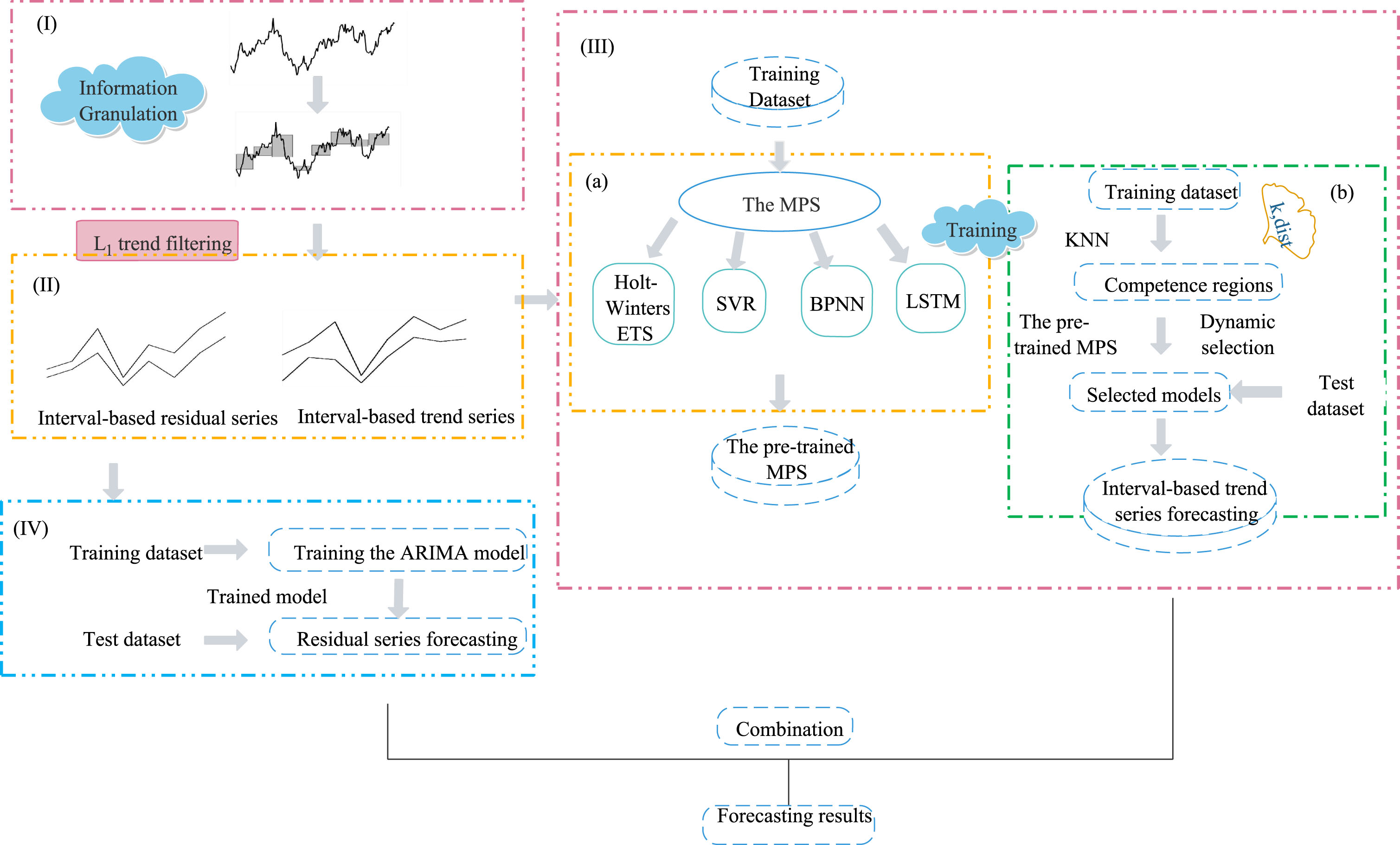
This study is to use a dynamic selection strategy to produce the desired predictive performance for interval-based trend series Y (t). In the training phase, it is vital to stress that using the training dataset trains each predictor in the MPS. The detailed training process for the MPS is introduced in the following subsection, and a brief procedure is described in Fig. 1(III)(a). Besides, considering the random fluctuation characteristics of residual series, the ARIMA model is utilized to forecast new pattern of residual series, as shown in Fig. 1(IV). The orders of AR(p) and MA(q) are chosen to forecast with the help of Akaike information criterion (AIC).

Fig. 1

Framework of the designed hybrid time series forecasting method based on information granulation and dynamic selection strategy.

3.1 The training process of multiple predictor system

Fig. 1(III)(a) presents the stage of model generation. Due to the superiority of the dynamic selection strategy, the MPS consists of four mainstream time series forecasting models: Holt-Winters exponential smoothing (Holt-Winters ETS) [9], support vector regression (SVR) [13], back propagation neural network (BPNN) [29] and long short-term memory (LSTM) network [15]. Four time series predictors in the MPS are trained on different datasets for the interval-based trend series. The parameters of predictors in the MPS are described in Table 1, which are associated with the model construction and influence dynamic selection. In this study, the values of model parameters are optimized by minimizing the root mean square error (RMSE). Besides, the parameter γ of the RBF kernel function is equal to the inverse of the lagged order L.

Table 1
The values of Parameters used in the MPS

Model Parameters Values

Holt-Winters ETS α (0,1]

β (0,1]

SVR Kernel function RBF

BPNN Units in hidden layer [10,20, 10,20]

Algorithm Adam

Activation function Sigmoid

The learning rate 0.001

Epoch 10000

LSTM Units in hidden layer [100,300]

Algorithm Adam

Model	Parameters	Values
Holt-Winters ETS	α	(0,1]
	β	(0,1]
SVR	Kernel function	RBF
BPNN	Units in hidden layer	[10,20, 10,20]
	Algorithm	Adam
	Activation function	Sigmoid
	The learning rate	0.001
	Epoch	10000
LSTM	Units in hidden layer	[100,300]
	Algorithm	Adam

The lagged order L means applying the previous L data to predict the test data. Aiming at different datasets, we are supposed to fix a suitable lagged order L for each predictor to alleviate the overfitting problem when training the MPS. With the guidance of structural risk minimization [30], the lagged order L of each predictive model in the MPS is defined in the following manners: $\underset{L}{argmin} \frac{\sum_{i = L + 1}^{N} | y_{i} - {\hat{y}}_{i} |}{N - L} C + λ \times L$ (8) where C, λ are penalty coefficients for controlling the balance between the ability of the model and model complexity, respectively; y_i and ${\hat{y}}_{i}$ are the real value and forecasting value of the i-th moment, respectively.

3.2 Dynamic selection and test process

The dynamic selection aims to select the most appropriate predictors for the local test pattern in dealing with the interval-based trend series Y (t). We can find a subset of training dataset similar to the test pattern, and there exist some differences between their forecasting values. These training samples are regarded as the competence region [31]. The competence regions can comprehensively evaluate individual models for test samples in the MPS. During the dynamic selection process, the competence region can be generated using the K-nearest neighbors (KNN) algorithm. The competence regions of each test pattern are the inputs of each pre-trained model in the MPS, and the average of the RMSE results is employed to identify the ideal model for predicting the test pattern. Different values of k may make a minor difference in forecasting performance. Thus we consider the average level of the forecasting accuracies of the FIGDS model with the different competence regions. In this study, the values of k are set to 1, 3, 5. The most suitable model from MPS for each test pattern can be identified by comparing RMSE values.

With regard to the test stage, a test input pattern of the trend series Y (t) = {Y_t-L+1, ⋯ , Y_t} is given, where L is the lagged order of the selected model from the MPS. Then, the test data Y_t+1’s forecasting value ${\hat{Y}}_{t + 1}$ is attained. The above-mentioned process is shown in Fig 1(III)(b).

4 Performance metrics of the hybrid time series forecasting method

In this study, we employ two classical evaluation indexes to measure the performance and forecasting accuracy of the FIGDS model.

4.1 Root mean square error (RMSE)

Root mean square error (RMSE) [32] is an important measure that generally appears in the literature to evaluate the forecasting performance of classical time series models. Because of obtaining interval-based information granules, RMSE can be calculated by

$RMSE = \sqrt{\frac{\sum_{j = 1}^{m} ({\hat{a}}_{j} - a_{j})^{2}}{m}} + \sqrt{\frac{\sum_{j = 1}^{m} ({\hat{b}}_{j} - b_{j})^{2}}{m}}$ (9) where $a_{j}, {\hat{a}}_{j}, b_{j}, {\hat{b}}_{j}$ are the lower bounds and upper bounds of the j-th information granule and predictive information granule, respectively; m represents the number of the predictive information granules.

4.2 Performance index of information granule

Since the outputs of the FIGDS model are a series of interval-based predictive information granules ${\hat{Ω}}_{1}, {\hat{Ω}}_{2}, \dots, {\hat{Ω}}_{m}$ , the forecasting performance of the FIGDS model can be measured by calculating the average value of coverage and specificity of the granular outputs [33], that is: $Q = Q_{1} \times Q_{2},$ (10) $Q_{1} = \frac{1}{m} \sum_{j = 1}^{m} cov (j),$ (11) $Q_{2} = \frac{1}{m} \sum_{j = 1}^{m} sp (j),$ (12) where $cov (j) = \frac{card {x_{k} | x_{k} \in {\hat{Ω}}_{j}}}{| s_{j} |}$ ;|s_j| is the cardinality of data contained in time series segment s_j; ${\hat{Ω}}_{j}$ is the j-th predictive information granule; $sp = \exp (- | \frac{{\hat{b}}_{j} - {\hat{a}}_{j}}{\max (s_{j}) - \min (s_{j})} |)$ ; max(s_j) and min(s_j) are the maximum and minimum values in time series segment s_j, respectively.

5 Experiments and results analysis

The outputs of the FIGDS model are interval information granules that can describe the variation ranges of future time series. Moreover, the designed method also offers a dynamic selection for forecasting tasks. In this section, experiments are carried out to highlight its effectiveness and practicality by comparison of the forecasting models without a dynamic selection strategy.

5.1 Experimental data description

The experiments are conducted on ten real-world time series datasets, which are respectively futures settlement price of WTI, Refined Oil Transportation Index (BCTI) and Sea Dry Bulk Index (BDI) both in Baltic Shipping, Shanghai Composite Index (SHCI), Shanghai Composite B Share Index, China Securities 100 Index, the closing price of COMEX gold, the closing price of the National Association of Securities Dealers Automated Quotations Index (NASDAQ), variation of atmospheric pressure in Beijing with time, temperature change in a region. The last two datasets all come from the UCI repository. A brief description of the ten time series datasets is shown in Table 2.

Table 2
Description of the ten time series datasets

Dataset Samples Date Numbers

Futures settlement price of WTI Training dataset 2000.1.4-2019.12.31 240

Test dataset 2020.1.2-2021.12.31 24

Refined Oil Transportation Index (BCTI) Training dataset 2002.1.2-2018.12.24 204

Test dataset 2019.1.2-2020.12.24 24

Sea Dry Bulk Index (BDI) Training dataset 2000.1.4-2018.12.24 228

Test dataset 2019.1.2-2020.12.24 24

Shanghai Composite Index (SHCI) Training dataset 2017.5.9-2019.12.31 643

Test dataset 2020.1.2-2020.1.23 22

Shanghai Composite B Share Index Training dataset 2000.1.4-2019.12.31 240

Test dataset 2020.1.2-2021.12.31 24

China Securities 100 Index Training dataset 2007.1.4-2020.12.31 168

Test dataset 2021.1.4-2021.12.31 12

The closing price of COMEX gold Training dataset 2000.1.5-2019.12.31 240

Test dataset 2020.1.2-2021.12.31 24

The closing price of NASDAQ Training dataset 2000.1.3-2018.12.31 240

Test dataset 2019.1.2-2019.12.31 24

Variation of atmospheric pressure in Beijing Training dataset 2010.1.1-2014.12.31 60

Test dataset 2015.1.1-2005.12.31 12

Temperature change in a region Training dataset 1981.1.1-1989.12.31 108

Test dataset 1990.1.1-1990.12.31 12

Dataset	Samples	Date	Numbers
Futures settlement price of WTI	Training dataset	2000.1.4-2019.12.31	240
	Test dataset	2020.1.2-2021.12.31	24
Refined Oil Transportation Index (BCTI)	Training dataset	2002.1.2-2018.12.24	204
	Test dataset	2019.1.2-2020.12.24	24
Sea Dry Bulk Index (BDI)	Training dataset	2000.1.4-2018.12.24	228
	Test dataset	2019.1.2-2020.12.24	24
Shanghai Composite Index (SHCI)	Training dataset	2017.5.9-2019.12.31	643
	Test dataset	2020.1.2-2020.1.23	22
Shanghai Composite B Share Index	Training dataset	2000.1.4-2019.12.31	240
	Test dataset	2020.1.2-2021.12.31	24
China Securities 100 Index	Training dataset	2007.1.4-2020.12.31	168
	Test dataset	2021.1.4-2021.12.31	12
The closing price of COMEX gold	Training dataset	2000.1.5-2019.12.31	240
	Test dataset	2020.1.2-2021.12.31	24
The closing price of NASDAQ	Training dataset	2000.1.3-2018.12.31	240
	Test dataset	2019.1.2-2019.12.31	24
Variation of atmospheric pressure in Beijing	Training dataset	2010.1.1-2014.12.31	60
	Test dataset	2015.1.1-2005.12.31	12
Temperature change in a region	Training dataset	1981.1.1-1989.12.31	108
	Test dataset	1990.1.1-1990.12.31	12

5.2 Hybrid time series forecasting for granular time series

In this part, we take the futures settlement price of WTI as an example to illustrate the detailed process of the FIGDS model. In the first process, the original time series of the futures settlement price of WTI is granulated by taking a month as a unit, following the principle of justifiable granularity. The granulation results, shown in Fig. 2(b), are more intuitive and keep the primary information in the original time series, as depicted in Fig. 2(a).

Table 3
Performance comparisons among different models (I)

Dataset Method RMSE Q Q ₁ Q ₂

Futures settlement price of WTI Holt-Winters ETS 82.7687

BPNN 12.4972

SVR 14.1901

LSTM 24.7438

ARIMA 57.8905

Holt-Winters ETS+ARIMA 111.60

BPNN+ARIMA 9.7743

SVR+ARIMA 11.2332

LSTM+ARIMA 23.7582

Mean_DS+ARIMA 8.5884

IG_Holt-Winters ETS+ARIMA 101.3902 0.0112 0.0326 0.3447

IG_SVR+ARIMA 12.3920 0.1623 0.2591 0.6266

IG_BPNN+ARIMA 11.0161 0.1857 0.3007 0.6176

IG_LSTM+ARIMA 15.3847 0.1551 0.2246 0.6904

FIGDS 9.2112 0.1861 0.2717 0.6847

Refined Oil Transportation Index (BCTI) Holt-Winters ETS 637.3040

BPNN 436.0732

SVR 338.3943

LSTM 360.0312

ARIMA 425.3838

Holt-Winters ETS+ARIMA 640.8412

BPNN+ARIMA 532.1675

SVR+ARIMA 333.3246

LSTM+ARIMA 356.5412

Mean_DS+ARIMA 247.8532

IG_Holt-Winters ETS+ARIMA 669.6300 0.1505 0.3472 0.4334

IG_SVR+ARIMA 387.8883 0.1552 0.3657 0.4162

IG_BPNN+ARIMA 512.3954 0.1157 0.2083 0.5555

IG_LSTM+ARIMA 416.0740 0.1734 0.3032 0.5719

FIGDS 261.5737 0.2082 0.4005 0.5199

Sea Dry Bulk Index (BDI) Holt-Winters ETS 4008.5

BPNN 789.5847

SVR 666.8283

LSTM 872.4484

ARIMA 997.1241

Holt-Winters ETS+ARIMA 3934.2

BPNN+ARIMA 771.8156

SVR+ARIMA 661.7089

LSTM+ARIMA 869.5184

Mean_DS+ARIMA 531.5312

IG_Holt-Winters ETS+ARIMA 3528.6 0.0127 0.0486 0.2608

IG_SVR+ARIMA 672.5922 0.1385 0.2315 0.5982

IG_BPNN+ARIMA 836.4104 0.1364 0.2477 0.5505

IG_LSTM+ARIMA 894.8885 0.0923 0.1574 0.5864

FIGDS 552.0646 0.1891 0.3241 0.5836

Shanghai Composite Index (SHCI) Holt-Winters ETS 105.0727

BPNN 36.0476

SVR 35.9261

LSTM 46.6751

ARIMA 132.7758

Holt-Winters ETS+ARIMA 105.1497

BPNN+ARIMA 33.3502

SVR+ARIMA 32.8540

LSTM+ARIMA 39.4780

Mean_DS+ARIMA 22.5379

IG_Holt-Winters ETS+ARIMA 102.1430 0.0210 0.0360 0.5847

IG_SVR+ARIMA 34.5516 0.2008 0.2008 0.5279

IG_BPNN+ARIMA 36.0042 0.2239 0.4242 0.5279

IG_LSTM+ARIMA 42.4205 0.1463 0.2254 0.6491

FIGDS 24.1657 0.2402 0.3807 0.6310

Shanghai Composite B Share Index Holt-Winters ETS 224.1978

BPNN 27.4148

SVR 22.0549

LSTM 36.2814

ARIMA 79.0476

Holt-Winters ETS+ARIMA 117.9506

BPNN+ARIMA 21.6146

SVR+ARIMA 23.5036

LSTM+ARIMA 45.2314

Mean_DS+ARIMA 13.2666

IG_Holt-Winters ETS+ARIMA 126.6204 0.0247 0.0978 0.2528

IG_SVR+ARIMA 22.7449 0.0657 0.0924 0.7111

IG_BPNN+ARIMA 19.3651 0.0626 0.0888 0.7049

IG_LSTM+ARIMA 40.9424 0.0867 0.1196 0.7251

FIGDS 12.7763 0.1487 0.2319 0.6411

Dataset	Method	RMSE	Q	Q ₁	Q ₂
Futures settlement price of WTI	Holt-Winters ETS	82.7687
	BPNN	12.4972
	SVR	14.1901
	LSTM	24.7438
	ARIMA	57.8905
	Holt-Winters ETS+ARIMA	111.60
	BPNN+ARIMA	9.7743
	SVR+ARIMA	11.2332
	LSTM+ARIMA	23.7582
	Mean_DS+ARIMA	8.5884
	IG_Holt-Winters ETS+ARIMA	101.3902	0.0112	0.0326	0.3447
	IG_SVR+ARIMA	12.3920	0.1623	0.2591	0.6266
	IG_BPNN+ARIMA	11.0161	0.1857	0.3007	0.6176
	IG_LSTM+ARIMA	15.3847	0.1551	0.2246	0.6904
	FIGDS	9.2112	0.1861	0.2717	0.6847
Refined Oil Transportation Index (BCTI)	Holt-Winters ETS	637.3040
	BPNN	436.0732
	SVR	338.3943
	LSTM	360.0312
	ARIMA	425.3838
	Holt-Winters ETS+ARIMA	640.8412
	BPNN+ARIMA	532.1675
	SVR+ARIMA	333.3246
	LSTM+ARIMA	356.5412
	Mean_DS+ARIMA	247.8532
	IG_Holt-Winters ETS+ARIMA	669.6300	0.1505	0.3472	0.4334
	IG_SVR+ARIMA	387.8883	0.1552	0.3657	0.4162
	IG_BPNN+ARIMA	512.3954	0.1157	0.2083	0.5555
	IG_LSTM+ARIMA	416.0740	0.1734	0.3032	0.5719
	FIGDS	261.5737	0.2082	0.4005	0.5199
Sea Dry Bulk Index (BDI)	Holt-Winters ETS	4008.5
	BPNN	789.5847
	SVR	666.8283
	LSTM	872.4484
	ARIMA	997.1241
	Holt-Winters ETS+ARIMA	3934.2
	BPNN+ARIMA	771.8156
	SVR+ARIMA	661.7089
	LSTM+ARIMA	869.5184
	Mean_DS+ARIMA	531.5312
	IG_Holt-Winters ETS+ARIMA	3528.6	0.0127	0.0486	0.2608
	IG_SVR+ARIMA	672.5922	0.1385	0.2315	0.5982
	IG_BPNN+ARIMA	836.4104	0.1364	0.2477	0.5505
	IG_LSTM+ARIMA	894.8885	0.0923	0.1574	0.5864
	FIGDS	552.0646	0.1891	0.3241	0.5836
Shanghai Composite Index (SHCI)	Holt-Winters ETS	105.0727
	BPNN	36.0476
	SVR	35.9261
	LSTM	46.6751
	ARIMA	132.7758
	Holt-Winters ETS+ARIMA	105.1497
	BPNN+ARIMA	33.3502
	SVR+ARIMA	32.8540
	LSTM+ARIMA	39.4780
	Mean_DS+ARIMA	22.5379
	IG_Holt-Winters ETS+ARIMA	102.1430	0.0210	0.0360	0.5847
	IG_SVR+ARIMA	34.5516	0.2008	0.2008	0.5279
	IG_BPNN+ARIMA	36.0042	0.2239	0.4242	0.5279
	IG_LSTM+ARIMA	42.4205	0.1463	0.2254	0.6491
	FIGDS	24.1657	0.2402	0.3807	0.6310
Shanghai Composite B Share Index	Holt-Winters ETS	224.1978
	BPNN	27.4148
	SVR	22.0549
	LSTM	36.2814
	ARIMA	79.0476
	Holt-Winters ETS+ARIMA	117.9506
	BPNN+ARIMA	21.6146
	SVR+ARIMA	23.5036
	LSTM+ARIMA	45.2314
	Mean_DS+ARIMA	13.2666
	IG_Holt-Winters ETS+ARIMA	126.6204	0.0247	0.0978	0.2528
	IG_SVR+ARIMA	22.7449	0.0657	0.0924	0.7111
	IG_BPNN+ARIMA	19.3651	0.0626	0.0888	0.7049
	IG_LSTM+ARIMA	40.9424	0.0867	0.1196	0.7251
	FIGDS	12.7763	0.1487	0.2319	0.6411

Table 4

Performance comparisons among different models (II)

Dataset	Method	RMSE	Q	Q ₁	Q ₂
China Securities 100 Index	Holt-Winters ETS	1762.9
	BPNN	879.2139
	SVR	565.1289
	LSTM	889.2399
	ARIMA	350.5036
	Holt-Winters ETS+ARIMA	1765
	BPNN+ARIMA	876.6421
	SVR+ARIMA	539.3152
	LSTM+ARIMA	885.0780
	Mean_DS+ARIMA	354.1871
	IG_Holt-Winters ETS+ARIMA	1437.1	0.0435	0.0725	0.6006
	IG_SVR+ARIMA	547.9714	0.1509	0.2246	0.6717
	IG_BPNN+ARIMA	873.5337	0.1323	0.1993	0.6639
	IG_LSTM+ARIMA	886.4154	0.1236	0.1957	0.6319
	FIGDS	346.3987	0.1956	0.3043	0.6428
The closing price of COMEX gold	Holt-Winters ETS	350.9350
	BPNN	112.0094
	SVR	105.8932
	LSTM	113.7111
	ARIMA	373.9328
	Holt-Winters ETS+ARIMA	356.3653
	BPNN+ARIMA	125.0193
	SVR+ARIMA	101.7293
	LSTM+ARIMA	107.4133
	Mean_DS+ARIMA	89.7068
	IG_Holt-Winters ETS+ARIMA	428.3260	0.0597	0.3841	0.1555
	IG_SVR+ARIMA	108.2825	0.2147	0.4185	0.5130
	IG_BPNN+ARIMA	117.7370	0.1327	0.1938	0.6846
	IG_LSTM+ARIMA	112.3549	0.1966	0.3098	0.6345
	FIGDS	100.4181	0.2271	0.4040	0.5621
The closing price of NASDAQ	Holt-Winters ETS	2259.7
	BPNN	1094.6
	SVR	567.1675
	LSTM	1031.7
	ARIMA	724.8003
	Holt-Winters ETS+ARIMA	2460.2
	BPNN+ARIMA	1085.7
	SVR+ARIMA	555.4310
	LSTM+ARIMA	1030.4
	Mean_DS+ARIMA	379.4480
	IG_Holt-Winters ETS+ARIMA	2688.4	0.0387	0.0833	0.4649
	IG_SVR+ARIMA	545.5318	0.2130	0.3254	0.6547
	IG_BPNN+ARIMA	1103	0.0931	0.1706	0.5458
	IG_LSTM+ARIMA	1044.2	0.1081	0.1786	0.6052
	FIGDS	396.3178	0.2369	0.3690	0.6420
Variation of atmospheric pressure in Beijing	Holt-Winters ETS	31.8697
	BPNN	6.9493
	SVR	12.2716
	LSTM	18.2981
	ARIMA	20.0543
	Holt-Winters ETS+ARIMA	32.5106
	BPNN+ARIMA	5.8600
	SVR+ARIMA	6.6606
	LSTM+ARIMA	18.3372
	Mean_DS+ARIMA	5.1057
	IG_Holt-Winters ETS+ARIMA	31.4134	0.2001	0.5685	0.3520
	IG_SVR+ARIMA	6.0694	0.2374	0.3383	0.7019
	IG_BPNN+ARIMA	6.2567	0.2340	0.3263	0.7174
	IG_LSTM+ARIMA	9.6595	0.2282	0.3295	0.6925
	FIGDS	5.3623	0.2982	0.4511	0.6609
Temperature change	Holt-Winters ETS	6.7577
	BPNN	4.8815
	SVR	5.6419
	LSTM	7.8910
	ARIMA	8.0836
	Holt-Winters ETS+ARIMA	8.2646
	BPNN+ARIMA	3.0474
	SVR+ARIMA	3.8354
	LSTM+ARIMA	2.4843
	Mean _ DS+ARIMA	2.2238
	IG_Holt-Winters ETS+ARIMA	7.2383	0.2184	0.3199	0.6826
	IG_SVR+ARIMA	4.1056	0.2975	0.4032	0.7378
	IG_BPNN+ARIMA	3.1095	0.3271	0.4543	0.7200
	IG_LSTM+ARIMA	3.3441	0.3127	0.4382	0.7137
	FIGDS	2.3801	0.3347	0.4651	0.7197

5.2.1 Extracting the trend of granular time series and experimental data division

Following the Fig. 1(II), L₁ trend filtering is employed to extract the potential trend of the granular time series of the futures settlement price of WTI. Additionally, the corresponding residual series can be gained by making the difference between the granular time series and the trend series. The parameter λ is set to 2. By observing Fig. 2(b) and (c), the L₁ trend filtering method can extract the linear trend in the futures settlement price of the WTI series. Moreover, the corresponding residual series is generated, as shown in Fig. 2(d). As shown in Table 1, the granular time series of the futures settlement price of WTI includes 240 training data and 24 test data.

Fig. 2

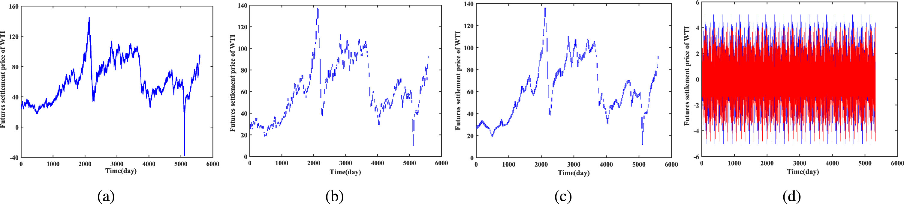
Futures settlement price of WTI:(a) The original time series; (b) The interval-based granular time series; (c) The interval-based trend series using L₁ trending filtering; (d) The residual time series.

5.2.2 Model training and dynamic selection

The upper bounds of the granular time series taken as an example are used for model training. In Fig. 1(IV), the residual series of the futures settlement price of WTI is stationary by the Augmented Dickey-Fuller (ADF) [34] test. With the help of the AIC, the autoregressive order p and the moving average q of the ARIMA model are fixed to 2 and 5, respectively. The ARIMA(2,0,5) model is employed for forecasting the residual series. Besides, we take four predictors to form MPS for forecasting for the trend series. By minimizing RMSE, the parameters of forecasting models can be determined. The α and β of the Holt-Winters ETS are both equal to 0.1; For the BPNN, a three-layer neural network with 19 nodes in the hidden layer is employed for forecasting tasks; The parameter γ of the RBF kernel function is equal to 0.5.

After obtaining the pre-trained MPS, we combine the competence regions and the dynamic selection strategy to choose the most suitable model for test pattern by comparing RMSE, as presented in Fig. 1(III)(b). Similar steps are used for the lower bound granular time series. Finally, the interval-based trend series prediction is completed for the futures settlement of WTI. For other experimental datasets, we can conduct the above-mentioned steps to establish the FIGDS model.

5.3 Analysis of experimental results

Guiding the evaluation index RMSE and the performance index Q of information granule, the forecasting performance of the FIGDS model is compared with the five single predictors Holt-Winters ETS, BPNN, SVR, LSTM and ARIMA. Other hybrid systems without dynamic selection strategy, including Holt-Winters ETS+ARIMA, SVR+ARIMA, BPNN+ARIMA, LSTM+ARIMA, Mean_DS+ARIMA, IG_ Holt-Winters ETS+ARIMA, IG_SVR+ARIMA, IG_BP NN+ARIMA and IG_LSTM+ARIMA, are conducted as comparative experiments. These comparative models are listed in Table 3 and Table 4. In Table 3, the inputs of the first ten models are the mean values time series and others are the interval granular time series. Fig. 3(a) and (b) correspond to the granulation results and the predictive performance of the futures settlement price of WTI on the test samples. We can observe that the generated predictive information granules are, to an extent, consistent with the original time series and offer future variation ranges.

Fig. 3

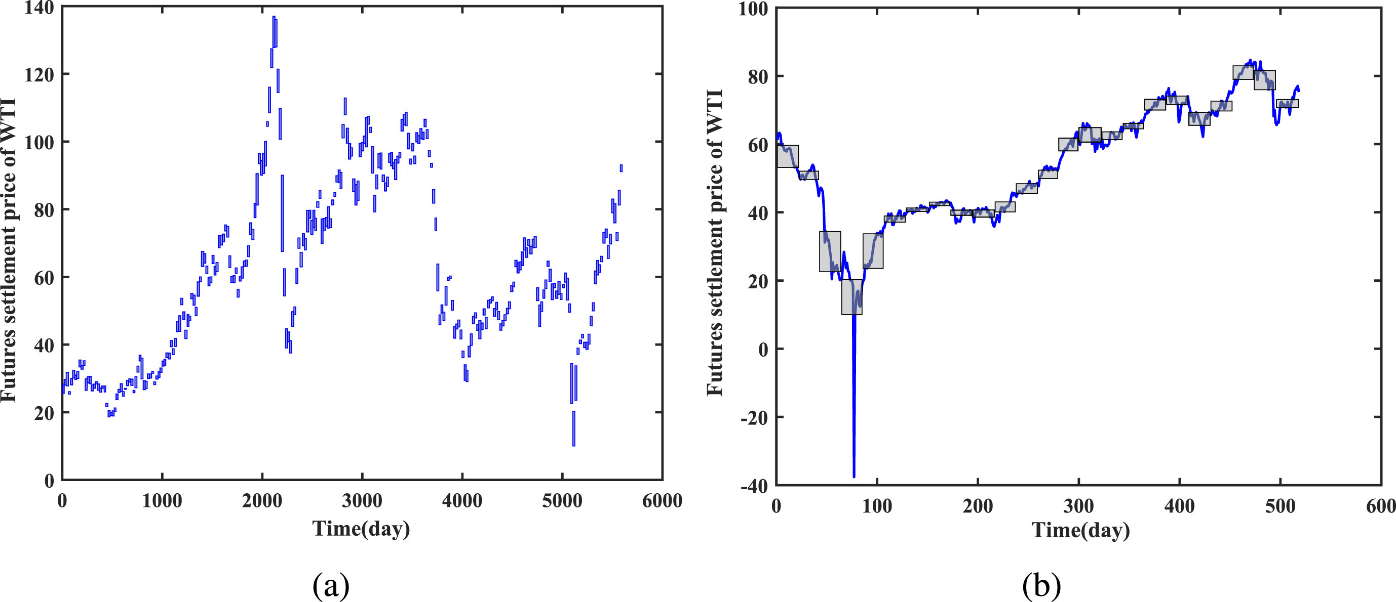
Prediction results of the hybrid method about futures settlement price of WTI: (a) The granulation results; (b) The forecasting results.

Table 3 and Table 4 present the empirical results of RMSE and Q. The lowest RMSE value and the highest Q value for each dataset are also highlighted in bold. By comparing the RMSE values on all datasets, we can observe that individual predictor is hard to achieve the best forecasting performance for all the cases. The FIGDS model can outperform the other models by some different margins.

Table 5

The Holm test

i	Forecasting method	$z_{i} = \frac{R_{i} - R_{0}}{SE}$	p _i	$\frac{α}{k - i}$
1	Holt-Winters ETS+ARIMA	6.1500	0.0000	0.0035
2	IG_Holt-Winters ETS+ARIMA	5.9000	0.0000	0.0038
3	Holt-Winters ETS	5.8000	0.0000	0.0041
4	ARIMA	4.5000	0.0000	0.0045
5	LSTM	4.0500	0.0000	0.0050
6	IG_LSTM+ARIMA	3.6000	0.0003	0.0056
7	BPNN	3.2500	0.0011	0.0062
8	LSTM+ARIMA	3.1000	0.0019	0.0071
9	IG_BPNN+ARIMA	2.700	0.0069	0.0083
10	BPNN+ARIMA	2.3500	0.0187	0.0100
11	SVR	2.1500	0.0315	0.0125
12	IG_SVR+ARIMA	1.8500	0.0643	0.0167
13	SVR+ARIMA	1.3500	0.1770	0.0250
14	Mean_DS+ARIMA	0.2500	0.8026	0.0500

The Friedman test [35] and the Holm test [36] are applied to examine the significant difference between the FIGDS model and other comparative models. In the Friedman test, the null hypothesis is that all models have the same performance based on their ranks in terms of RMSE. The value of the $χ_{F}^{2}$ is 109.3, while the critical value is 23.68 at the significance level α = 0.05. Thus, the null hypothesis is rejected, which means that all models have significant differences in forecasting accuracy. R_i, R₀ are the average rank of the i-th forecasting model and the FIGDS model, respectively, and SE is equal to 2 in Table 5. Following the Holm step-down procedure, the tenth null-hypothesis can not be rejected and all the remaining hypotheses are retained. That is, the FIGDS model is significantly different with Holt-Winters ETS, BPNN, LSTM, ARIMA, Holt-Winters ETS+ARIMA, LSTM+ARIMA, IG_Holt-Winters ETS+ARIMA, IG_BPNN+ARIMA and IG_LSTM+ARIMA and has no significant difference in BPNN+ARIMA, SVR, IG_SVR+ARIMA and Mean_DS+ARIMA.

Due to the interval information granules as the final outputs, the average level of coverage Q₁ and specificity Q₂ are also taken as performance indicators. We observe from Table 3 and Table 4 that the Q₁ is smaller when the Q₂ is larger and vice versa, which reflects the conflicting relationship between coverage and specificity. The FIGDS model exhibits sound performances compared to IG_Holt-Winters ETS+ARIMA, IG_SVR+ ARIMA, IG_BPNN+ARIMA, and IG_LSTM +ARIMA in terms of the Q. The comparisons also illustrate that the outputs of the FIGDS model are more representative. The FIGDS model realizes a trade-off between the future variation ranges and forecasting accuracy when compared with the model on mean values time series.

6 Conclusions

This study designs a hybrid time series forecasting (FIGDS) model based on information granulation and dynamic selection strategy. The method first translates the original time series into granular time series following the principle of justifiable granularity, retaining the primary information in the numerical time series. Predictive systems are established by considering the granular trend and residual item. The dynamic selection strategy selects the most appropriate models for the trend series test pattern. The ARIMA model achieves the forecasting of the residual series. The results of two predictive systems form interval information granules to reflect variation ranges of future time series. The proposed model can reach promising forecasting accuracy than other comparative models and is feasible for forecasting real-world time series.

References

Nayak

S.C.

, Misra

B.B.

and Behera

H.S.

, An adaptive second order neural network with genetic-algorithm-based training (ASONN-GA) to forecast the closing prices of the stock market, International Journal of Applied Metaheuristic Computing 7(2) (2016), 39–57.

Katris

, A time series-based statistical approach for outbreak spread forecasting: Application of COVID-19 in Greece Expert Systems with Applications, 166 (2021). https://doi.org/10.1016/j.eswa.2020.114077.

Niu

, Wang

and Zhang

, Carbon price forecasting system based on error correction and divideconquer strategies, Applied Soft Computing 118 (2022), https://doi.org/10.1016/j.asoc.2021.107935.

Hussain

, Hussain

, Khan

A.A.

, Naqvi

S.A.A.

and Jamil

, A deep learning approach for hydrological time-series prediction: A case study of Gilgit river basin, Earth Science Informatics 13(3) (2020), 915–927.

Fan

F.G.

, Yu

, Dong

S.Q.

, Yeh

Y.H.

, Hong

Fore-casting short-term electricity load using hybrid support vector regression with grey catastrophe and random forest modeling, Utilities Policy. https://doi.org/10.1016/j.jup.2021.10129.

Kitagawa

and Gersch

, A smoothness priors time-varying AR coefficient modeling of nonstationary covariance time series, IEEE Transactions on Automatic Control 30(1) (2021), 48–56.

Chen

J.F.

, Wang

W.M.

and Huang

C.M.

, Analysis of an adaptive time-series autoregressive moving-average (ARMA) model for short-term load forecasting, Electric Power Systems Research 34(3) (1995), 187–196.

Newbold

, ARIMA model building and the time series analysis approach to forecasting, Journal of Forecasting 2(1) (1983), 23–35.

Maia

A.L.S.

and Maia

F.D.A.T.D.

, Holt’s exponential smoothing and neural network models for forecasting intervalvalued time series, International Journal of Forecasting 27(3) (2011), 740–759.

10.

Engle

R.F.

, Autoregressive conditional heteroscedasticity with estimates of the variance of United Kingdom inflation, Econometrica 50 (1982), 987–1007.

11.

Bollerslev

, Generalized autoregressive conditional heteroscedasticity, Journal of Econometrics 31 (1986), 307–327.

12.

Muhammad

E.R.

, Simon

S.P.

and Venkateswaran

P.R.

, Day-ahead forecasting of solar photovoltaic output power using multilayer perceptron, Neural Computing and Applications 28(12) (2017), 3981–3992.

13.

Cao

L.J.

and Tay

F.E.H.

, Support vector machine with adaptive parameters in financial time series forecasting, IEEE Transactions on Neural Networks 14(6) (2003), 1506–1518.

14.

Akdi

, Gölveren

, Ünlü

K.D.

and Yücel

M.E.

, Modeling and forecasting of monthly PM2.5 emission of Paris by periodogram-based time series methodology, Environmental Monitoring and Assessment 193(10) (2021), 307–327.

15.

Fischer

and Krauss

, Deep learning with long short-term memory networks for financial market predictions, European Journal of Operational Research 270(2) (2018), 654–669.

16.

Yao

, Dai

and Song

, Several novel dynamic ensemble selection algorithms for time series prediction, Neural Processing Letters 50(2) (2018), 1789–1829.

17.

, Hao

, Feng

Q.Q.

, Sun

and Liu

, Optimal selection of heterogeneous ensemble strategies of time series forecasting with multi-objective programming, Expert Systems with Applications 116 (2022). https://doi.org/10.1016/j.eswa.2020.114091.

18.

, Gao

, Suganthan

P.N.

and Wang

D.Z.W.

, Bayesian optimization based dynamic ensemble for time series forecasting, Information Sciences 591 (2022), 155–175.

19.

Pedrycz

, Hirota

, Pedrycz

and Dong

, Granular representation and granular computing with fuzzy sets, Fuzzy Sets and Systems 203 (2012), 17–32.

20.

Zadeh

L.A.

, Fuzzy sets and information granularity, Advances in Fuzzy Set Theory and Applications 11 (1979), 3–18 4830–4839.

21.

Pedrycz

and Homenda

, Building the fundamentals of granular computing: A principle of justifiable granularity, Applied Soft Computing 13(10) (2013), 4209–4218.

22.

Guo

H.Y.

, Pedrycz

and Liu

L.D.

, Hidden markov models based approaches to long-term prediction for granular time series, IEEE Transactions on Fuzzy Systems 26(5) (2018), 2807–2817.

23.

Wang

W.N.

, Pedrycz

and Liu

X.D.

, Time series long-term forecasting model based on information granules and fuzzy clustering, Engineering Applications of Artificial Intelligence 41 (2015), 17–24.

24.

Guo

H.Y.

, Wang

L.D.

, Liu

X.D.

and Pedrycz

, Trend-based granular representation of time series and its application in clustering, IEEE Transactions on Cybernetics 99 (2021), 1–10.

25.

Kim

S.J.

, Koh

, Boyd

and Gorinevsky

, L1 trend filtering, SIAM Review 51(2) (2009), 339–360.

26.

Leser

C.E.V.

, A simple method of trend construction, Journal of the Royal Statistical Society 21(1) (1961), 91–107.

27.

Duan

, Yu

, Pedrycz

, Wang

and Yang

, Time-series clustering based on linear fuzzy information granules, Applied Soft Computing 73 (2018), 1053–1067.

28.

Makridakis

and Hibon

, ARMA models and the Box-Jenkins methodology, Journal of Forecasting 16(3) (1997), 147–163.

29.

Hosseini

H.G.

, Luo

and Reynolds

K.J.

, The comparison of different feed forward neural network architectures for ECG signal diagnosis, Medical Engineering & Physics 28(4) (2006), 372–378.

30.

Vapnik

, Principles of risk minimization for learning theory, Advances in Neural Information Processing Systems 4 (1991), 831–838.

31.

Sergio

A.T.

, de Lima

T.P.F.

, Ludermir

T.B

, Dynamic selection of forecast combiners, Neurocomputing 218 (2016), 37–50.

32.

Gupta

K.K.

and Kumar

, Hesitant probabilistic fuzzy set based time series forecasting method, Granular Computing 4(4) (2019), 739–758.

33.

Ouyang

T.H.

, Pedrycz

and Pizzi

N.J.

, Rule-based modeling with DBSCAN-based information granules, IEEE Transactions on Cybernetics 99 (2019), 1–11.

34.

Harris

R.I.D.

, Testing for unit roots using the augmented Dickey-Fuller test: Some issues relating to the size, power and the lag structure of the test, Economics Letters 38(4) (1992), 381–386.

35.

Friedman

, The use of ranks to avoid the assumption of normality implicit in the analysis of variance, Journal of the American Statistical Association 32(200) (1937), 675–701.

36.

Demsar

, , Statistical comparisons of classifiers over multiple data sets, The Journal of Machine Learning Research 7 (2006), 1–30.