In this paper, the second-order fuzzy homogeneous differential equation is transformed into a more special simplest form under the condition that the solution of the boundary value problem of the equation exists and is unique. Then the eigenvalues of the boundary value problem of the second-order simplest fuzzy homogeneous differential equation are studied and the theorems that make the eigenvalues exist are proposed and then illustrated with examples. Finally, it is proved that when the second-order fuzzy coefficient in the second-order fuzzy homogeneous differential equation is a fuzzy number, the solution set of its corresponding second-order granular homogeneous differential equation becomes larger, that is, the solution set of fuzzy differential equations with real numbers is a subset of the solution set with fuzzy coefficients as fuzzy numbers.
Fuzzy differential equations (FDEs), first proposed by Kandel in 1978 [17], are equations with uncertain conditions, coefficients or parameters, which are commonly used to model the propagation of epistemic uncertainty in dynamical environments, and fuzzy numbers are often used to express the uncertainty in these equations. By solving FDEs, practical problems with uncertain factors in many fields such as physics, control theories and neural networks can be solved. The research of FDEs focuses on the study of the properties of solutions, that is, existence, uniqueness, periodicity and so on. The properties of solutions can well explain the long-term reflection of the model in the dynamic environment with uncertain phenomena.
As we all know, the concept of fuzzy derivative is indispensable when defining fuzzy differential equations. However, in view of the particularity of fuzzy number subtraction, that is, the difference between two fuzzy numbers after subtraction is not necessarily a fuzzy number, so the definition of fuzzy derivative is facing difficulties and it is always a challenge for researchers to solve fuzzy differential equations. In recent years, in order to overcome this difficulty, researchers have sought a variety of methods to study FDEs. After 30 years of development, the study of FDEs has formed three types: ZEP-type(see [7, 28]), DI-type(see [3, 15],etc) and H-type(see[1, 16], etc). Additionally, more applications and studies of fuzzy differential equations are listed in references [18] and [21].
In 1997, Zadeh put forward the idea of fuzzy information granulation for the first time in the literature [30], pointing out that granulation of object A is actually a collection of gathered points. W.Pedrycz pointed out that granular computing imitated the thinking mode of human beings to granulate abstract data. In accordance with the idea of dividing complex problems into simple problems at different levels, various information granules at different levels were obtained through information granulation, and then different granular characteristics were observed [4, 23].
The idea of granular computing is also applicable to solving fuzzy differential equations. In 2018, Mazandarani proposed a new method to study FDEs in [19], which is called granular differentiability. By introducing relative distance measure variable αx and membership degree μ, the abstract fuzzy differential equation is transformed into concrete granular differential equation, and the characteristics of each granular differential equation can be discussed in layers. This method solves some difficult problems in solving FDEs in the past and makes us have a thorough reform in solving FDEs. We do not need to consider the monotony of the supporting closure length of the solution, nor do we need to consider the non-natural behavior phenomenon and the pairing of these problems in the modeling. It not only overcomes the disadvantages of the previous methods, but also inherits the advantages of the previous methods, and provides great convenience for solving FDEs. It can not be ignored that the application of granular differentiability of fuzzy-number-valued-function provides great convenience in solving practical mathematical problems(see [2, 29]).
In this paper, we aim to study a class of second-order FDEs with fuzzy parameter , i.e.,
where is a fuzzy numerical function, is the first-order granule derivative, is the second-order granule derivative and , , are the corresponding coefficients respectively. The idea of granular differentiability is applied to granulate the fuzzy differential equation. In other words, the abstract fuzzy differential equation (1.1) is transformed into a differential equation with multiple information granules. We can explore the solution of the differential equation under each information granule and finally get the information of the solution of the fuzzy differential equation.
The paper is organized as follows. In Section 2, we introduce some definitions and theorems of fuzzy numbers and granular derivatives. In Section 3, we demonstrate in detail how to transform the second-order homogeneous FDE into the simplest form. In Section 4, we solve the eigenvalues of homogeneous BVP for the simplest second order FDEs. Meanwhile, two examples, corresponding diagram descriptions and some new definitions are given. Our conclusions are given in Section 5.
Preliminaries
The symbols encountered in this paper show that “-" stands for subtraction in real number sense, “+" for addition in real number sense, “⊖" for subtraction in fuzzy sense, “⊕” for addition in fuzzy sense, “⊙" for number multiplication in fuzzy sense and “⊗" for multiplication in fuzzy sense.
Definition 2.1 Denote
is a fuzzy number space, where
(1) is normal, i.e., there exists an such that
(2) is fuzzy convex, i.e., for any and 0≤ μ ≤ 1 ;
(3) is upper semi-continuous;
(4) is compact.
Here, cl (X) denotes the closure of set X. For 0 < μ ≤ 1, the μ-level set of (or simply the μ-cut) is defined by The core of is the set of elements of having membership grade 1, i.e., .
Definition 2.2 ([19]) Let be a fuzzy number. The horizontal membership function ugr : [0, 1] × [0, 1] → [a, b] is a representation of as ugr (μ, αu) = x in which “gr" stands for the granule of information included in x ∈ [a, b] , μ ∈ [0, 1] is the membership degree of x in is called RDM variable, and .
The horizontal membership function of triangular fuzzy numbers , then, . The horizontal membership function of trapezoidal fuzzy numbers , .
Definition 2.3 ([19]) The horizontal membership function of is also denoted by . Moreover, using
the μ-level sets of the vertical membership function of , which is in fact the span of the information granule, can be obtained.
Definition 2.2 and Definition 2.3 are difficult to understand intuitively, so an example is given to help us understand.
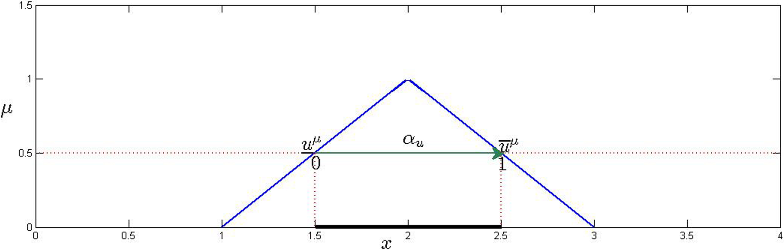
Example 2.1 For , the vertical membership function is expressed as follows,
when μ = 0.5, then μ-level sets is [1.5, 2.5].
According to Definition 2.2, the horizontal membership function of is , μ ∈ [0.1] , αu ∈ [0.1]. Next, let’s consider the case when μ = 0.5, , αu ∈ [0.1]. Here, we focus on αu,
By observing the above expressions, it is noticed that the value of is also changing during the range from αu = 0 to αu = 1, and the change process from to is gradual. Therefore, when αu takes the value in [0, 1], takes every value in the μ-level sets [1.5, 2.5] with membership degree μ = 0.5. Crucially, each resulting is called an “information granule".(See Figure 2.1)
The triangular fuzzy number .
Definition 2.4 ([19]) Two fuzzy numbers and are said to be equal if and only if for all αu = αv ∈ [0, 1] , and μ ∈ [0, 1].
Definition 2.5 ([19]) Let and be two fuzzy numbers whose horizontal membership functions are ugr (μ, αu) and vgr (μ, αv), respectively, and “⊙gr” denotes one of the four basic operations, i.e., addition, subtraction, multiplication and division. Then, is a fuzzy number such that . It should be noted 0 ∉ vgr (μ, αv) when “⊙gr” denotes the division operator.
Note 2.1 ([19]) Let . Then, always presents μ-level sets of the fuzzy number .
Note 2.2 ([19]) The difference between two fuzzy numbers defined in Definition 2.5 is called granular difference (gr-difference).
Definition 2.6 ([19]) Based on RDM fuzzy interval arithmetic, the following relations hold for :
(1) ;
(2) ;
(3) ; and
(4)
Definition 2.7 ([19]) Let . The function , is a distance between two fuzzy numbers and .
Note 2.3 ([19]) The metric space (E1, Dgr) is called granular metric on the space of fuzzy numbers.
Theorem 2.1([19]) The metric space (E1, Dgr) is a complete metric space.
Definition 2.8 ([19]) Let includes n ∈ N distinct fuzzy numbers . The horizontal membership function of at the point t ∈ [a, b] is denoted by , and defined as in which αf ≜ (αu1, αu2, ⋯ , αun) are the RDM variables corresponding to the fuzzy numbers.
Definition 2.9 ([19]) The fuzzy function is said to be granular differentiable at the point t ∈ [a, b] if there exists a fuzzy number , such that the following limit exists:
The limit is taken in the metric space (E1, Dgr).
Definition 2.10 ([19]) Let mapping be a continuous fuzzy function whose horizontal membership function, i.e., fgr (t, μ, αf) is integrable on t ∈ [a, b]. Let denotes the integral of on [a, b]. Then, the fuzzy function is said to be granular integrable on [a, b] if there exists a fuzzy number such that .
Note 2.4 ([19]) Suppose the fuzzy function mapping is gr-differentiable, and is continuous on [a, b], then, .
Definition 2.11 The fuzzy function is said to be granular differentiable at the point t ∈ [a, b], and f is first order granular differentiable. If there exits a fuzzy number , such that the following limit exists:
The limit is taken in the metric space (E1, Dgr).
Theorem 2.2(See [19] Theorem 5) The fuzzy function is gr-differentiable at the point t ∈ [a, b] if and only if its horizontal membership function is differentiable with respect to t at that point. Moreover,
Theorem 2.3The fuzzy function is gr-differentiable at the point t ∈ [a, b], and is first order granular differentiable if and only if its horizontal membership function is first order granular differentiable at that point. Moreover,
Transforming the second-order homogeneous FDEs into the simplest form
Using the granular derivative and horizontal membership function of fuzzy numerical function, the second-order homogeneous FDE is transformed into the simplest form after many transformations. The detailed transformation process is as follows.
The general form of our second-order homogeneous FDE is as follows,
Through Theorem 2.3, (3.1) is transformed as follows,
We select the following appropriate variable transformation,
Both sides of equation (3.3) are multiplied by function ggr (t, μ, αx) at the same time,
Let’s make
Let’s make
Then
where μ ∈ [0, 1], αx ∈ [0, 1], t ∈ [a, b].
Firstly, the coefficient of is changed to 1. In fact, as long as the independent variable transformation is introduced,
(t should be represented by ξgr). Secondly, the transformations of independent variables and unknown functions are introduced,
We continue to substitute the expression of into (3.3) as follows,
To further simplify, we can choose kgr so that (kgr) 4rgrpgr = 1 and then , so that the equation (3.3) can be simplified into the following form,
Therefore, (3.5) is called the simplest second-order fuzzy homogeneous differential equation.
Solving the eigenvalues of homogeneous BVP for the simplest second order FDEs
Consider the following second order linear fuzzy differential equation with fuzzy parameters,
where αx ≜ (αx1, αx2, αx3, αx4) .
Definition 4.1 The fuzzy homogeneous boundary value problem consisting of (4.1) and (4.2) with fuzzy parameter “" is called the fuzzy eigenvalue problem.
Note 4.1 The granular homogeneous boundary value problem consisting of (4.5) and (4.6) with parameter “λgr" is called the granular eigenvalue problem.
Definition 4.2 is called the fuzzy eigendeterminant of fuzzy eigenvalue problems.
Note 4.2 Δ (λgr) is called the granular eigendeterminant of granular eigenvalue problems.
Definition 4.3 The fuzzy eigendeterminant determined by causes (4.1) to have a solution, which is called the fuzzy eigenvalue.
Note 4.3 The eigendeterminant Δ (λgr) determined by λgr causes (4.5) to have a solution, which is called the granular eigenvalue.
Theorem 4.1The necessary and sufficient condition for the existence of a unique solution to a fuzzy homogeneous boundary value problem composed of (4.1) and (4.2) is that there exists a unique solution to the homogeneous boundary value problem of a granular differential equation composed of (4.5) and (4.6).
Theorem 4.2If and are the two linearly independent solutions of the granular differential equation (4.5). Let nonempty sets
when A∩ B ≠ ∅ and A = B, for a given μ, αx, both ∃x0, y0 ∈ A ∩ B, we have x0 - y0 = 0, which x0 ∈ A, y0 ∈ B. Namely,
Then the solutions to boundary value problems (4.5) and (4.6) exist and are unique.
As can be seen from Theorem 4.2, the following theorems can be deduced, so that the homogeneous boundary value problem of the simplest second-order fuzzy differential equation has eigenvalue.
Theorem 4.3The homogeneous boundary value problem of fuzzy homogeneous differential equation composed of (4.1) and (4.2) has eigenvalue if and only if the homogeneous boundary value problem of granular homogeneous differential equation composed of (4.5) and (4.6) has eigenvalue.
Theorem 4.4In order for the homogeneous boundary value problem of homogeneous differential equation composed of (4.5) and (4.6) to have eigenvalues, it must be satisfied,
Proof. It can be obtained from (4.5),
then
namely
Obviously, it is difficult to solve the eigenvalue λgr we need in (4.8), so we further convert (4.8) to the form (4.9). However, when we solve the eigenvalue λgr through (4.9), we find it difficult to get an explicit expression. Here, an implicit expression can be expressed as λgr = λgr (μ, αx), where αx ≜ (αx1, αx2, αx3, αx4). It’s clear that the value of λgr only depends on μ and αx.
Example 4.1 Let us consider the homogeneous boundary value problem of a second order FDEs with a fuzzy parameter known as ,
According to Theorem 2.3, there is
According to (4.12),
In order to have a solution to the granular homogeneous boundary value problem composed of (4.12) and (4.13), the conditions in Theorem 4.2 must be satisfied. The following
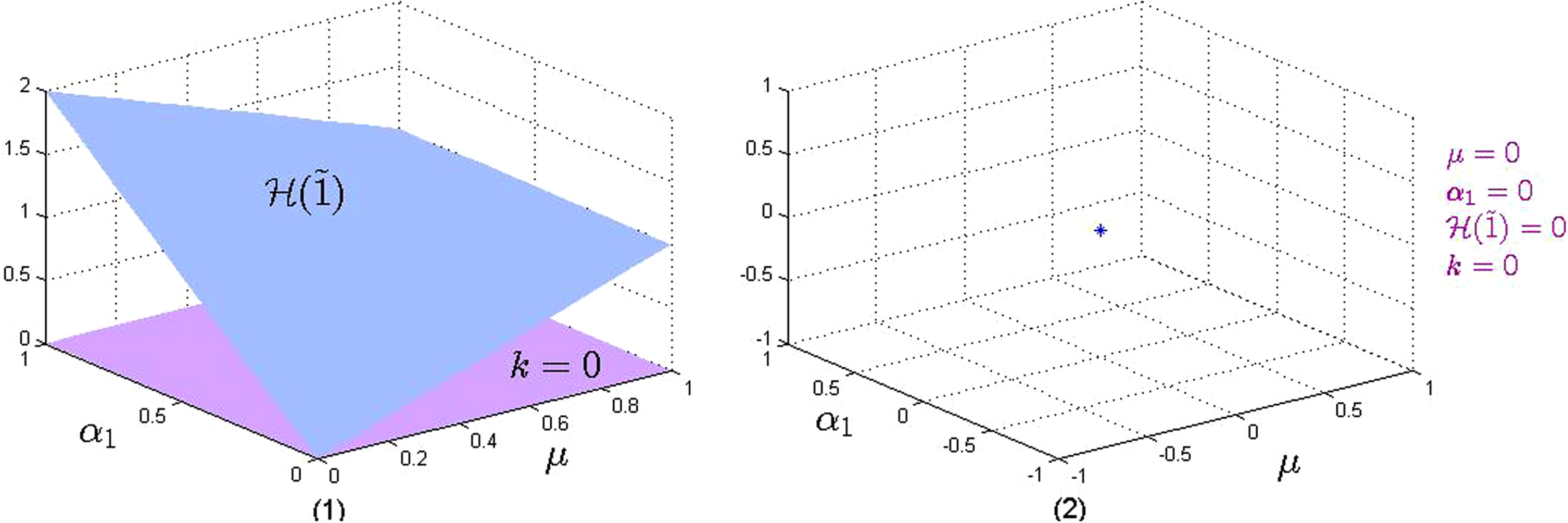
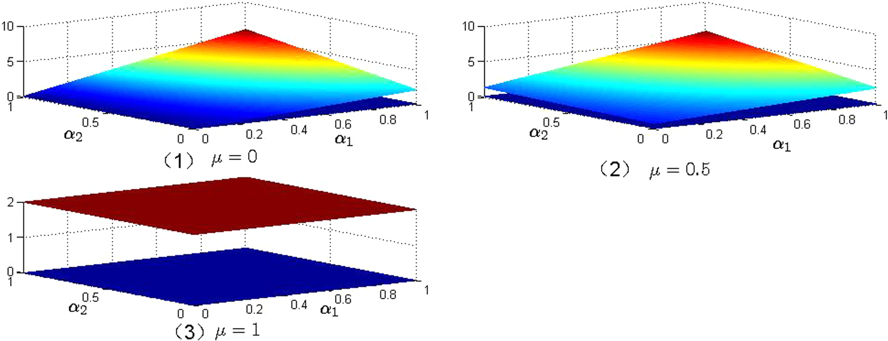
where k = 0, 1, 2, ⋯ , μ ∈ [0, 1] , α1 ∈ [0, 1] . More importantly, the left and right sides of Equation (4.15) must be kept identical. Next, we will observe how μ and α1 on the left change according to the value of k on the right, so as to keep the left and right sides of Equation (4.15) identical.
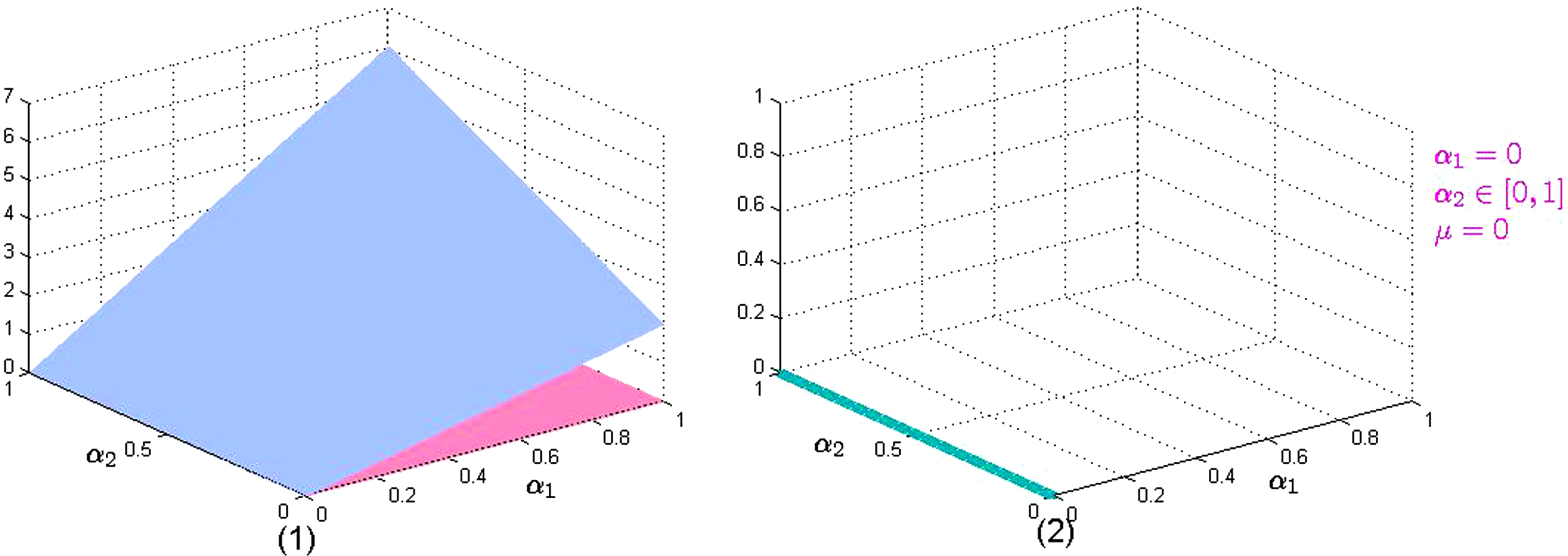
When k = 0, then μ + 2 (1 - μ) α1 = 0. It can be seen from (2) in Fig 4.1 that the left and right sides of Equation (4.15) are identical only when μ = 0 and α1 = 0. Only in this way can the homogeneous boundary values of granular composed of (4.12) and (4.13) be guaranteed to have a solution. When μ ∈ (0, 1] and α1 ∈ (0, 1], there is no guarantee that the homogeneous boundary value of granular composed of (4.12) and (4.13) has a solution.
The intersection of the horizontal membership function and the plane k = 0.
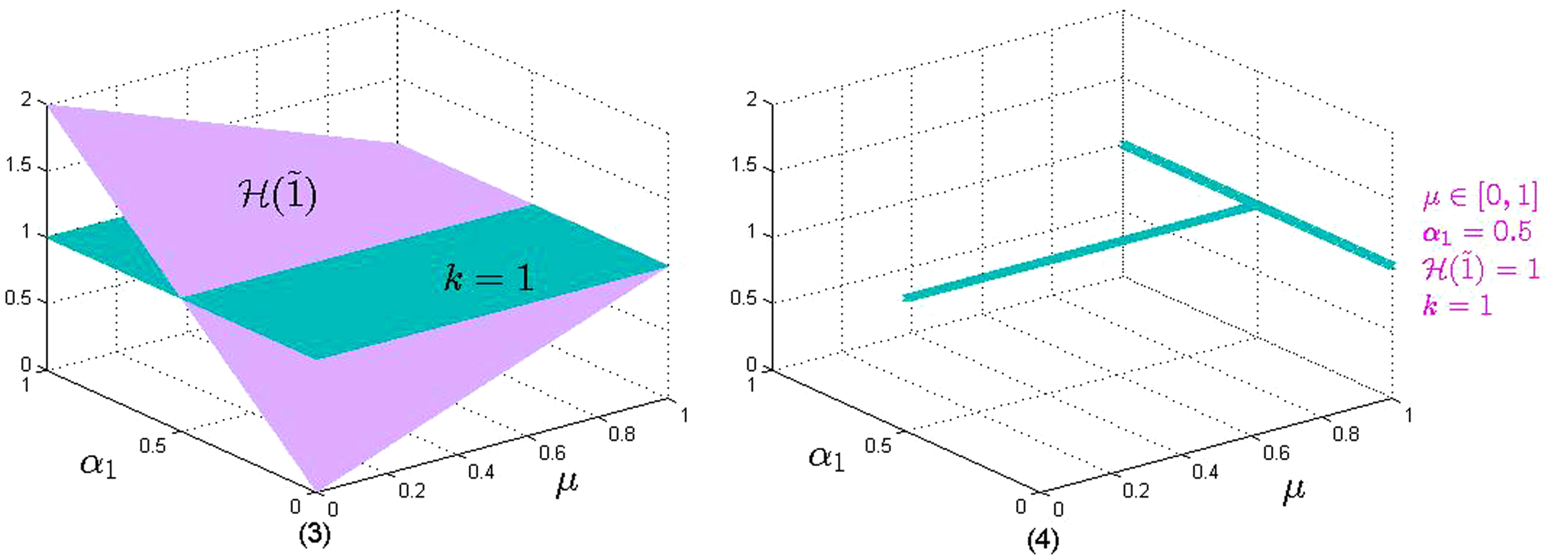
When k = 1, then μ + 2 (1 - μ) α1 = 1. It can be seen from (2) in Fig 4.2 that the left and right sides of Equation (4.15) are identical only when μ ∈ [0, 1] and α1 = 0.5. Only in this way can the homogeneous boundary values of granular composed of (4.12) and (4.13) be guaranteed to have a solution. When μ ∈ [0, 1] and α1 ∈ [0, 0.5) ∪ (0.5, 1], there is no guarantee that the homogeneous boundary value of granular composed of (4.12) and (4.13) has a solution.
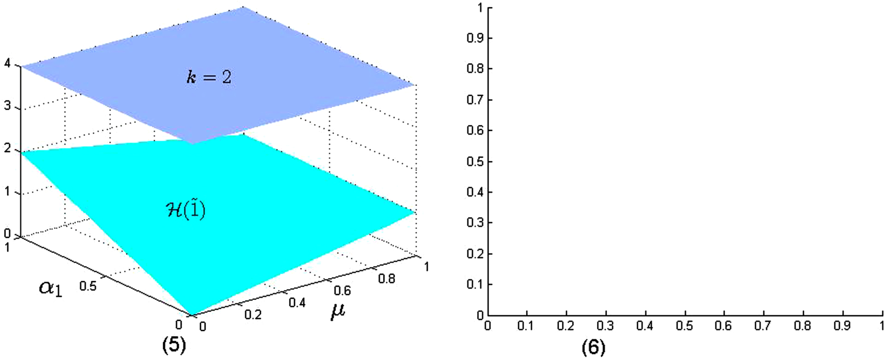
When k = 2, then μ + 2 (1 - μ) α1 = 4. As can be seen from Fig. 4, no matter any values of μ and α1 are taken, the left and right sides of Equation (4.15) are not identical. Then the granular homogeneous boundary value problem composed of (4.12) and (4.13) has no solution. It can be seen from the case of k = 2 that the left and right sides of Equation (4.15) cannot be identical at k = 3, 4, ⋯.
The intersection of the horizontal membership function and the plane k = 1.
The intersection of the horizontal membership function and the plane k = 2.
To sum up, it is only when k = 0 and k = 1 that the left and right sides of Equation (4.15) are always identical through further values of μ ∈ [0, 1] and α1 ∈ [0, 1]. When k = 0 or k = 1, we can only take some individual values of μ and α1 such that the granular homogeneous boundary value problem composed of (4.12) and (4.13) has a solution. But that doesn’t satisfy Theorem 3.1. Therefore, the fuzzy homogeneous boundary value problem composed of (4.10) and (4.11) has no solution.
Example 4.2 Let’s consider the homogeneous BVP of a second-order FDE with unknown fuzzy parameter ,
According to Theorem 2.3, there is
In order to have a solution to the granular homogeneous BVP composed of (4.18) and (4.19), the conditions in Theorem 4.1 must be satisfied. The following
When μ takes each of the values of [0,1] (i.e., μ is given), the intersection of plane M with plane K = 0.
When μ = 0, the intersection of plane M with plane K = 0.
According to Fig 4.4 and Fig 4.5, when μ, α1 and α2 meet the conditions of μ = 0, α1 = 0 and α2 ∈ [0, 1], the left and right sides of Equation (4.20) can be made identical.
Similarly, when μ ∈ (0, 1], α1 ∈ (0, 1] and α2 ∈ [0, 1], then μ (1 + μ) +2μα2 (1 - μ) +2α1 (1 - μ2) +4α1
α2 (1 - μ2) ≠0. We have
Case 3:
It can be seen from case 2 that case 3 is satisfied for μ = 0, α1 = 0 and α2 ∈ [0, 1].
From the three cases above, different conditions must be required for μ, α1 and α2 to make the left and right sides of Equation (4.22) identical. In each case, the granular homogeneous boundary value problem composed of (4.18) and (4.19) can be solved, but the fuzzy homogeneous boundary value problem composed of (4.16) and (4.17) has no solution.
It can be known from the above discussion that the second-order fuzzy coefficient in the second-order fuzzy differential equation (4.1) has always been treated as a real number 1. Furthermore, we consider the fuzzy coefficient as a fuzzy number. Therefore, when the range of the coefficient changes from real number to fuzzy number, what will happen to the second-order fuzzy differential equation we solved and its second-order fuzzy differential equation with eigenvalue problem.
When (where ), consider a simple second-order fuzzy differential equation, that is,
From (4.1) to (4.5), that is, (4.23) can be transformed as follows,
Case 1: If μ + 2α1 (1 - μ) ≠0 (where μ ∈ (0, 1] , α1 ∈ (0, 1]), then (4.24) can be organized as:
The granular differential equation (4.24) has a corresponding basic solutions group.
Case 2: If μ + 2α1 (1 - μ) =0 (where μ = 0, α1 = 0), obviously, the corresponding granular differential equation (4.24) has an infinite number of solutions. There are countless granules of information xgr at the same time.
We can see that when , the solution set of the second-order granular differential equation (4.24) corresponding to the second-order fuzzy differential equation (4.23) becomes larger and the number of solutions increase obviously. Furthermore, we notice that when , the solution of fuzzy differential equation (4.23) is just the Case 1. Therefore, when the second-order fuzzy coefficient changes from a real number to a fuzzy number, the corresponding solution sets of the second-order granular differential equations have inclusion relations. That is to say, in the corresponding fuzzy differential equation, it is a special case that is a real number and is a fuzzy number.
Of course, it is worth noting that the solution xgr obtained by (4.25) is a part of the solution obtained by (4.24). In essence, we can think of “xgr" as a “granule" here.
Conclusions
In this study, we find that when studying fuzzy differential equations in the sense of granular differentiability, there must be two closely related variables, namely, the membership degree μ and RDM variable αu. When μ ∈ [0, 1] and αu ∈ [0, 1], the second-order fuzzy differential equation and the second-order granular differential equation can be transformed. And we will encounter different situations, that is, when the range of μ and αu is only a subset of [0, 1], we can also transform fuzzy differential equations into granular differential equations. In addition, we also study the conditions for μ and αu in fuzzy differential equations with fuzzy parameters to make the fuzzy parameters become fuzzy eigenvalues. Finally, we find that the solution set of fuzzy differential equations with real numbers is a subset of the solution set with fuzzy coefficients as fuzzy numbers.
However, for the second order linear fuzzy differential equation with fuzzy parameters, we can solve the eigenvalues of homogeneous BVP for the simplest second order FDEs according to the Theorems 4.1-4.4 proposed in this paper. But in fact, since the randomness of parameters combinations to solve the eigenvalues of homogeneous BVP for the simplest second order FDEs, it is pretty difficult to solve concrete examples and we can only give some very simple examples in our paper.
The following example is used to illustrate the difficulties encountered and further research plans.
Example 5.1 Let’s consider the homogeneous BVP of a second-order FDE with unknown fuzzy parameter ,
According to the Theorem 2.3, there is
According to (4.12),
In order to obtain the solution of the granular homogeneous boundary value problem composed of (4.12) and (4.13), the conditions in the Theorem 4.2 must be satisfied. The following
namely
Representing in terms of triangular fuzzy numbers, then
then
where μ ∈ [0, 1], α
λ ∈ [0, 1], α1 ∈ [0, 1] .
In the following three cases, the left and right sides of the equation must intersect:
(1) let μ = 1, then
(2) let μ = 0, α
λ = 0, then
(3) let α
λ = 0, α1 = 0, then
As mentioned above, parameters μ, α1, and α
λ in equation 5.1 all vary randomly within the interval [0, 1]. The variation of parameters and the limitation of the domain of the tangent function itself make a pretty complicated situation after taking the tangent function of the equation 5.2, so only three special cases can be discussed here. The more general situation is the main target of our further research.
Footnotes
Acknowledgments
This work is supported by National Natural Science Foundation of China (NO. 12161082, 12061067) and Natural Science Foundation of Gansu Province (21JR7RA134). The authors are very grateful to the anonymous referees for their valuable suggestions.
References
1.
AgarwalR.P., LakshmikanthamV. and NietoJ.J., On the concept of solution for fractional differential equations with uncertainty, Nonlinear Anal72 (2010), 2859–2862.
2.
AgarwalR.P., BaleanuD., NietoJ.J., TorresD.F.M. and ZhouY., A survey on fuzzy fractional differential and optimal control nonlocal evolution equations, Journal of Computational and Applied Mathematics339 (2018), pp. 3–29.
3.
AbbasbandyS., NietoJ.J. and AlaviM., Tuning of reachable set in one dimensional fuzzy differential inclusions, Chaos Soliton Fract26 (2005), 1337–1341.
4.
BargielaA. and PedryczW., Granular Computing: An Introduction, Kluwer Academic Publishers, Dordrecht, 2003.
5.
BargielaA. and PedryczW., Toward a theory of Granular Computing for human-centered information processing, IEEE Transactions on Fuzzy Systems16(2) (2008), pp. 320–330.
6.
BedeB. and GalS.G., Generalizations of the differentibility of fuzzy number value functions with applications to fuzzy differential equations, Fuzzy Sets Syst151 (2005), 581–599.
7.
CecconelloM.S., BassaneziR.C., BrandãoA.J.V. and LeiteJ., On the stability of fuzzy dynamical systems, Fuzzy Sets Syst248 (2014), 106–121.
8.
ChenM., FuY., XueX. and WuC., Two-point boundary value problems of undamped uncertain dynamical systems, Fuzzy Sets Syst159 (2008), 2077–2089.
9.
ChenM., WuC., XueX. and LiuG., On fuzzy boundary value problems, Inf Sci178 (2008), 1877–1892.
10.
CecconelloM.S., LeiteJ., BassaneziR.C. and BrandãoA.J.V., Invariant and attractor sets for fuzzy dynamical systems, Fuzzy Sets Syst265 (2015), 99–109.
11.
Chalco-CanoY. and Román-FloresH., Comparation between some approaches to solve fuzzy differential equations, Fuzzy Sets Syst160 (2009), 1517–1527.
12.
KhatuaD., MaityK. and KarS., A fuzzy production inventory control model using granular differentiability approach, SOFT COMPUTING25(4) (2020), 2687–2701.
13.
DeA., KhatuaD. and KarS., Control the preservation cost of a fuzzy production inventory model of assortment items by using the granular differentiability approach, Computational and Applied Mathematics39 (2020), 285.
14.
DiamondP. and KloedenP., Metric Spaces of Fuzzy Sets, World Scientific, Singapore, 1994.
15.
HllermeierE., An approach to modeling and simulation of uncertain dynamical systems, Int J Uncertainty Fuzziness Knowl Based Syst5 (1997), 117–137.
16.
IssaM.S.B., HamoudA.A. and GhadleK.P., Numerical solutions of fuzzy integro-differential equations of the second kind, Journal of Mathematics and Computer Science23(1) (2021), pp. 67–74.
17.
KandelA. and ByattW.J., Fuzzy differential equations, in Proc Int Conf Cybern Soc (1978), 1213–1216.
MazandaraniM., ParizN. and KamyadA.V., Granular Differentiability of Fuzzy-Number-Valued Functions, IEEE Trans Fuzzy Syst26 (2018), 310–323.
20.
MazandaraniM. and ParizN., Sub-optimal control of fuzzy linear dynamical systems under granular differentiability concept, ISA Trans76 (2018), 1–17.
21.
MazandaraniM. and XiuL., A Review on Fuzzy Differential Equations, IEEE ACCESS9 (2021), 62195–62211.
22.
Witold. Pedrycz, Granular Computing for Data Analytics: A Manifesto of Human-Centric Computing, IEEE/CAA JOURNAL OF AUTOMATICA SINICA5 (2018), 1025–1034.
23.
PedryczW. and GacekA., Temporal granulation and its application to signal analysis, Information Sciences143 (2002), pp. 1–4, 47-71.
24.
MazandaraniM. and ZhaoY., Fuzzy bang-bang control problem under granular differentiability, J Franklin Inst355 (2018), 4931–4951.
25.
NajariyanM. and ZhaoY., Fuzzy fractional quadratic regulator problem under granular fuzzy fractional derivatives, IEEE Trans Fuzzy Syst26 (2018), 2273–2288.
26.
NajariyanM., ParizN. and VuH., Fuzzy linear singular differential equations under granular differentiability concept, Fuzzy Sets and Systems429 (2022), pp. 169–187.
27.
OberguggenbergerM., Fuzzy and weak solutions to differential equations, in: Proceedings of the Tenth International Conference IPMU 2004, Perugi Editrice Universite, La Sapienza, Italy, 2004, pp. 517–524.
28.
OberguggenbergerM. and PittschmannS., Differential equations with fuzzy parameters, Math Comput Model Dyn Syst5 (1999), 181–202.
29.
YangH., WangF. and GongZ., Solving the BVP to a class of second-order linear fuzzy differential equations under granular differentiability concept, Journal of Intelligent and Fuzzy Systems42(6) (2022), pp. 5483–5499.
30.
ZadehL.A., Toward a theory of fuzzy information granulation and its centrality in human reasoning and fuzzy logic, Fuzzy Sets Syst90 (1997), 111–127.