Gene selection in a gene decision space with application to gene expression data classification

Abstract

Gene selection is an important research topic in data mining. A gene decision space means a real-valued decision information system (RVDIS) where objects, conditional attributes and information values are cells, genes and gene expression values, respectively. This paper explores gene selection in a gene decision space based on information entropy and considers its application for gene expression data classification. In the first place, the distance between two cells in a given decision subspace is constructed. In the next place, the binary relations induced by this decision subspace are defined. After that, some information entropy for a gene decision space are investigated. Lastly, several gene selection algorithms in a gene decision space are presented by using the presented information entropy. The presented algorithms are applied to gene expression data classifications. Multiple publicly available gene expression datasets are employed to evaluate the gene selection performances of the proposed algorithms, while two commonly-used classifiers, KNN and CART, are utilized to obtain 10 fold cross validation accuracy of classification (ACC). The classification results demonstrated that the proposed algorithms can lower significantly the number genes selected, achieve the higher ACC, and outperform the other competing methods, such as raw data, Fisher, tSNE, PCA, FMIFRFS and DNEAR, with respect to gene number and ACC.

Keywords

Gene expression data Gene decision space Gene selection Uncertainty measurement

1 Introduction

1.1 Research background and related works

Uncertainty can be found almost everywhere. Uncertainty measurement (UM) has been the research content in various fields, such as machine learning [49], pattern recognition [8, 18], image processing [28], medical diagnosis [23, 46] and data mining [13].

Rough set theory (RST) is an effective tool to handle uncertainty. An information system (IS) in the light of RST was presented by Pawlak [29]. Most applications of RST, such as uncertainty modeling [9], reasoning with uncertainty, rule extraction [6, 43], classification and gene selection [19, 41] are related to an IS.

Information entropy is also an essential tool for estimating uncertainty [31]. Some contributions have been made in this respect. For example, Wierman [43] presented UM in RST; Beaubouef et al. [5] proposed a method for measuring the uncertainty of a rough set. Li et al. [26] studied the uncertainty of a fuzzy relation IS; Zhang et al. [52] gave UM for a fully fuzzy IS; Tan et al. [40] considered entropy measure for intuitionistic fuzzy information; Singh et al. [36] proposed a fuzzy similarity-based rough set approach aiming at selecting attributes in the background of a set-valued IS;

Feature selection or attribute reduction as an essential way of data processing technology in machine learning can effectively lessen redundant feature and improve classification accuracy. Many researchers studied feature selection. Jain et al. [16] first defined intuitionistic fuzzy relations, fuzzy lower and upper approximations, and parameterized intuitionistic fuzzy granule, then defined the dependency degree measure of attributes, finally presented a feature selection based on intuitionistic fuzzy rough sets, FMIFRFS. The experimental results showed that FMIFRFS could obtain better feature subsets. Sun et al. [39] studied feature selection based on neighborhood entropy rough sets. The feature selection first defined uncertainty measures in a neighborhood decision information system, then described neighborhood credibility, neighborhood coverage degrees and mutual information, finally presented a decision neighborhood entropy-based attribute reduction, DNEAR. The experimental results demonstrated that DNEAR could acquire better feature subset and classification accuracy. Additionally, Zeng et al. [53] investigated incremental feature selection on a hybrid IS by using fuzzy rough set method; Cornelis et al. [9] studied a general definition for a fuzzy decision reduct; Wang et al. [45] presented feature selection algorithm from the angle of iterative; Li et al. [24] explored information entropy based feature selection for heterogeneous data. Wang et al. [44] put forward local conditional entropy based feature selection; Jia et al. [21] proposed similarity-based feature selection in RST from clustering perspective; Dai et al. [11] discussed information entropy based feature selection in an interval-valued IS; Hu et al. [20] gave a robust and fast feature selection method on the basis of separability for a fuzzy decision IS.

Abdi and Williams [4] presented Principal Component Analysis (PCA). It is a commonly used dimensionality reduction method. Its essence is to perform a basic transformation in linear space to maximize the variance of the transformed data projected on new coordinate axes.

Van der Maaten and Hinton [42] proposed t-Distributed Stochastic Neighbor Embedding (tSNE). It is also a commonly used dimensionality reduction method. It converts the similarity between data points into probability, and converts into the probability based on Gaussian distribution in high-dimensional space whereas converts into the probability based on t-distribution in the embedded space (two-dimensional space). Unlike PCA, tSNE is a nonlinear dimensionality reduction method.

1.2 Motivation and contributions

DNA expresses deoxyribonucleic acid. In biology, DNA is the primary genetic matter and contains genetic information about living organisms. There are many genes on each DNA molecule, and genes are DNA fragments with genetic effects. The phenomenal expansion of the biological data expressing DNA information provides a driving force to address biological problems. Biological data can be expressed by gene expression data. By performing gene selection method, it can eliminate high-level noises and redundant genes for original gene expression data. For instance, Sharma et al. [35] proposed a gene selection method for cancer classification based on multi-objective meta-heuristic machine learning algorithms; Sun et al. [38] presented joint neighborhood entropy-based gene selection method with fisher score for tumor classification; Bommertet et al. [7] gave a filter method for feature selection of high-dimensional gene expression data; Sheng al. [33] proposed a feature selection method for high-dimensional single cell gene expression data based on unsupervised learning; Li al. [22] studied Gaussian kernel based gene selection in a single cell gene decision space. However, the selection of the best genes using traditional statistical analysis and machine learning methods often leads to a dimensional disaster. Thus, we need to lessen the complexity of gene expression data and to establish a gene selection theory. Information entropy is an effective method to deal with gene selection.

If information values in an IS are real numbers, then it can be called a real-valued information system (RVIS). An RVIS with decision attributes is a real-valued decision information system (RVDIS). If objects, conditional attributes and information values in an RVDIS respectively are cells, genes and gene expression values, then this RVDIS is said to be a gene decision space.

Based on the above research motivation, the major contributions are summarized as follows.

(1) Traditional rough set model can only deal with discrete or classified data. For gene expression data with real or noisy data, discrete preprocessing commonly used may lose part information of the data itself, which lessens the accuracy of classification or clustering. This study does not use discrete preprocessing for gene expression data, but utilizes the distance between two gene expression values to define the tolerance relation in a gene decision space, where a variable parameter is introduced to control this distance.

(2) By means of the defined tolerance relation in a gene decision space, this study constructs the tolerance class as an information granule. Based on an information granule, conditional information entropy is introduced. Moreover, this study presents several gene selection algorithms in a gene decision space by means of the introduced conditional information entropy.

(3) The presented algorithms are applied to gene expression data classifications. The classification results show that these algorithms can effectively select suitable genes related to classifications, and can significantly improve the classification performance.

1.3 Organization

The flowchart of this study is illustrated in Fig. 1.

Fig. 1

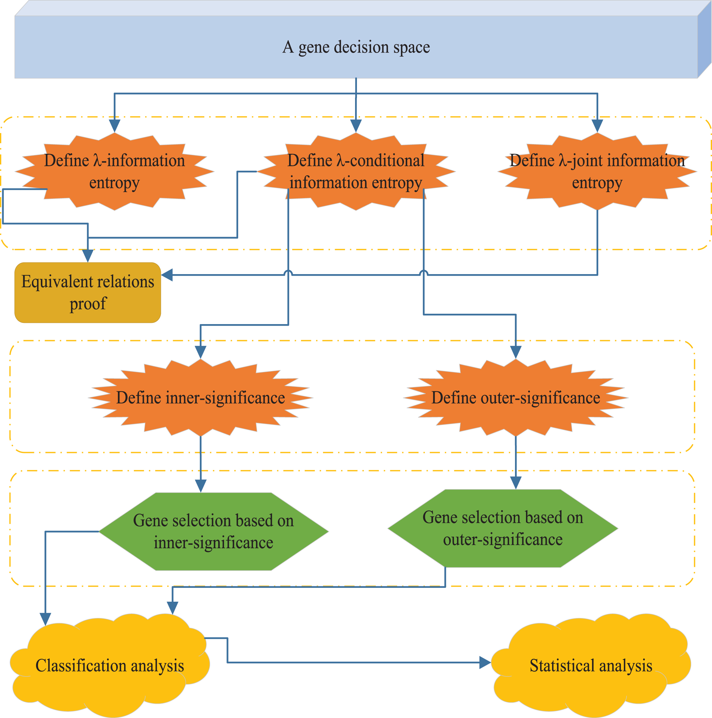
Flowchart of this study

The remaining part of this study is organized as follows. In Section 2, we define a gene decision space and tolerance relations. In Section 3, we introduce some general information entropy in a gene decision space. In Section 4, we investigate the gene selection ratio, inner-significance and outer-significance in a gene decision space and design gene selection algorithms based on inner-significance and outer-significance. In Section 5, we apply the designed gene selection algorithms to gene expression data classifications. In Section 6, we summarize this study.

2 Preliminaries

In this study, O, 2^O and |X| indicate a finite set, the collection of all subsets of O and the number of elements in X ∈ 2^O, respectively. Put $O = {o_{1}, o_{2}, \dots, o_{n}}$ (2.1)

2.1 A gene decision space

(O, C ∪ {d}) is referred to as a real-valued decision information system (RVDIS), if ∀ a ∈ C, ∀ o ∈ O, a (o) is a real number, where C is the conditional attribute set and d is a decision attribute.

Definition 2.1. [22] Let (O, C ∪ {d}) be an RVDIS where O is the cell set and C is the gene set to describe the cells. Then (O, C ∪ {d}) is called a gene decision space, if ∀ a ∈ C, ∀ o ∈ O, a (o) means the gene expression value of o with respect to a,

Moreover, if P ⊆ C, then (O, P ∪ {d}) is said to be a decision subspace of (O, C ∪ {d}).

From the above definition, we can see that a gene decision space is a special RVDIS in essence, where objects are cells, conditional attributes are genes to describe the cells, and the information value a (o) is the gene expression value of the cell o with respect to the gene a.

2.2 Tolerance relations in a gene decision space

T is said to be a binary relation on O whenever T ⊆ O × O. Moreover, if ∀ o ∈ O, (o, o) ∈ T, then T is said to be reflexive; if (o, o′) ∈ T implies (o′, o) ∈ T, then T is said to be symmetric; if T is reflexive and symmetric, T is said to be tolerance.

Definition 2.2. [22] Let (O, C ∪ {d}) be a gene decision space. ∀ a ∈ C, ∀ o, o′ ∈ O, the distance between a (o) and a (o′) is defined as $d (a (o), a (o^{'})) = \frac{| a (o) - a (o^{'}) |}{\hat{a}}$ (2.2) where $\hat{a} = \max {a (x) : x \in O} - \min {a (x) : x \in O} .$

Remark 2.3. [22] In (2.2), if $\hat{a} = 0$ , then $d (a (o), a (o^{'})) = 0$ (2.3)

Definition 2.4. Let (O, C ∪ {d}) be a gene decision space with P ⊆ C and λ ∈ [0, 1]. Define $R_{P}^{λ} = {(o, o^{'}) \in O \times O : \forall a \in P, d (a (o), a (o^{'})) \leq λ}$ (2.4) $T_{d} = {(o, o^{'}) \in O \times O : d (o) = d (o^{'})}$ (2.5)

Clearly, $R_{P}^{λ}$ is a tolerance relation on O.

Denote $R_{P}^{λ} (o) = {o^{'} \in O : (o, o^{'}) \in R_{P}^{λ}}$ (2.6) $T_{d} (o) = {o^{'} \in O : (o, o^{'}) \in T_{d}}$ (2.7) Then $R_{P}^{λ} (o)$ and T_d (o) are said to be to the tolerance and decision classes of o, respectively.

Put $O / T_{d} = {T_{d} (o) : o \in O} = {D_{1}, D_{2}, \dots, D_{r}}$ (2.8)

Proposition 2.5. Let (O, C ∪ {d}) be a gene decision space. Then the following properties hold:

(1) If P₁ ⊆ P₂ ⊆ C, then ∀ λ ∈ [0, 1], ∀ o ∈ O, $R_{P_{2}}^{λ} (o) \subseteq R_{P_{1}}^{λ} (o);$

(2) If 0 ≤ λ₁ ≤ λ₂ ≤ 1, then ∀ P ⊆ C, ∀ o ∈ O, $R_{P}^{λ_{1}} (o) \subseteq R_{P}^{λ_{2}} (o) .$

Proof. (1) Obviously, $R_{P_{1}}^{λ} (o) = ⋂_{a \in P_{1}} {o^{'} \in O : d (a (o), a (o^{'})) \leq λ},$ $R_{P_{2}}^{λ} (o) = ⋂_{a \in P_{2}} {o^{'} \in O : d (a (o), a (o^{'})) \leq λ},$ Since P₁ ⊆ P₂, we have $R_{P_{2}}^{λ} (o) \subseteq R_{P_{1}}^{λ} (o) .$

(2) Obviously, $R_{P}^{λ_{1}} (o) = ⋂_{a \in P} {o^{'} \in O : d (a (o), a (o^{'})) \leq λ_{1}},$ $R_{P}^{λ_{2}} (o) = ⋂_{a \in P} {o^{'} \in O : d (a (o), a (o^{'})) \leq λ_{2}},$ Since λ₁ ≤ λ₂, we have $R_{P}^{λ_{1}} (o) \subseteq R_{P}^{λ_{2}} (o) .$ □

Definition 2.6. Let (O, C ∪ {d}) be a gene decision space. Given P ⊆ C and λ ∈ [0, 1]. $\partial_{P}^{λ} : O \to 2^{V_{d}}$ is defined as $\partial_{P} (o) = d (R_{P}^{λ} (o))$ (2.9) Then $\partial_{P}^{λ}$ is referred to as generalized decision in (O, P ∪ {d}).

Moreover, if ∀ o ∈ O, |∂_C (o) |=1, then (O, C ∪ {d}) is said to be λ-consistent; otherwise, it is said to be λ-inconsistent.

Proposition 2.7. Assume that (O, C ∪ {d}) is a gene decision space with λ ∈ [0, 1], P ⊆ C and o ∈ O. Then

$R_{P}^{λ} (o) \subseteq T_{d} (o) \Leftrightarrow | \partial_{P}^{λ} (o) | = 1 .$

Proof. “ ⇒ ". Let $R_{P}^{λ} (o) \subseteq T_{d} (o)$ . Suppose $z \in \partial_{P}^{λ} (o)$ . Then there exists $y \in R_{P}^{λ} (o)$ such that z = d (y). $y \in R_{P}^{λ} (o)$ implies that y ∈ T_d (o). So z = d (y) = d (u). Thus $| \partial_{P}^{λ} (o) | = 1 .$

“⟸”. Let $| \partial_{P}^{λ} (o) | = 1$ . Suppose $y \in R_{P}^{λ} (o)$ . Then $d (y) \in \partial_{P}^{λ} (o)$ . Since $d (o) \in \partial_{P}^{λ} (o)$ and $| \partial_{P}^{λ} (o) | = 1$ , we have d (o) = d (y). Then y ∈ T_d (o). Thus $R_{P}^{λ} (o) \subseteq T_{d} (o)$ . □

Corollary 2.8. Assume that (O, C ∪ {d}) is a gene decision space with λ ∈ [0, 1] and P ⊆ C. Then

$R_{P}^{λ} \subseteq T_{d} \Leftrightarrow \forall o \in O, | \partial_{P}^{λ} (o) | = 1 .$

Proof. It follows from Proposition 2.7. □

Theorem 2.9. Let (O, C ∪ {d}) be a gene decision space with λ ∈ [0, 1]. Then (O, C ∪ {d}) is λ-consistent ⇔ $R_{C}^{λ} \subseteq T_{d} .$

Proof. It follows from Corollary 2.8. □

3 Entropy measure for a gene decision space

Definition 3.1. Suppose that (O, C ∪ {d}) is a gene decision space with P ⊆ C and λ ∈ [0, 1]. Then λ-information entropy of P is defined as $H^{λ} (P) = - \sum_{i = 1}^{n} \frac{| R_{P}^{λ} (o_{i}) |}{n} {log}_{2} \frac{| R_{P}^{λ} (o_{i}) |}{n}$ (3.1)

Proposition 3.2. Assume that (O, C ∪ {d}) is a gene decision space with P ⊆ C and λ ∈ [0, 1]. Then

$0 \leq H^{λ} (P) \leq n {log}_{2} n .$

Proof. Note that ∀ i, $1 \leq | R_{P}^{λ} (o_{i}) | \leq n$ . Then $\frac{1}{n} \leq \frac{| R_{P}^{λ} (o_{i}) |}{n} \leq 1,$ $0 \leq - {log}_{2} \frac{| R_{P}^{λ} (o_{i}) |}{n} \leq {log}_{2} n .$

Then $0 \leq - \frac{| R_{P}^{λ} (o_{i}) |}{n} {log}_{2} \frac{| R_{P}^{λ} (o_{i}) |}{n} \leq {log}_{2} n .$

By Definition 3.1, $0 \leq H^{λ} (P) \leq n {log}_{2} n .$ □

Definition 3.3. Let (O, C ∪ {d}) be a gene decision space with P ⊆ C and λ ∈ [0, 1]. Then λ-conditional information entropy of P to d is defined as $H^{λ} (P | d) = - \sum_{i = 1}^{n} \sum_{j = 1}^{r} \frac{| R_{P}^{λ} (o_{i}) \cap D_{j} |}{n} {log}_{2} \frac{| R_{P}^{λ} (o_{i}) \cap D_{j} |}{| R_{P}^{λ} (o_{i}) |}$ (3.2)

Proposition 3.4. Assume that (O, C ∪ {d}) is a gene decision space.

(1) If P ⊆ Q ⊆ C, then ∀ λ ∈ [0, 1], $H^{λ} (Q | d) \leq H^{λ} (P | d) .$

(2) If 0 < λ₁ ≤ λ₂ ≤ 1, then ∀ P ⊆ C, $H^{λ_{1}} (P | d) \leq H^{λ_{2}} (P | d) .$

Proof. (1) ∀ i, j, denote $p_{ij}^{(1)} = | R_{P}^{λ} (o_{i}) \cap D_{j} |, p_{ij}^{(2)} = | R_{P}^{λ} (o_{i}) \cap (O - D_{j}) |;$ $q_{ij}^{(1)} = | R_{Q}^{λ} (o_{i}) \cap D_{j} |, q_{ij}^{(2)} = | R_{Q}^{λ} (o_{i}) \cap (O - D_{j}) | .$

By Proposition 2.5, we have $\forall i, R_{Q}^{λ} (o_{i}) \subseteq R_{P}^{λ} (o_{i}) .$

Clearly, $0 \leq q_{ij}^{(1)} \leq p_{ij}^{(1)}, 0 \leq q_{ij}^{(2)} \leq p_{ij}^{(2)},$ $p_{ij}^{(1)} + p_{ij}^{(2)} = | R_{P}^{λ} (o_{i}) |, q_{ij}^{(1)} + q_{ij}^{(2)} = | R_{Q}^{λ} (o_{i}) | .$

Then $\begin{matrix} H^{λ} (P | d) & = - \sum_{i = 1}^{n} \sum_{j = 1}^{r} \frac{| R_{P}^{λ} (o_{i}) \cap D_{j} |}{n} {log}_{2} \frac{| R_{P}^{λ} (o_{i}) \cap D_{j} |}{| R_{P}^{λ} (o_{i}) |} \\ = - \sum_{i = 1}^{n} \sum_{j = 1}^{r} \frac{p_{ij}^{(1)}}{n} {log}_{2} \frac{p_{ij}^{(1)}}{p_{ij}^{(1)} + p_{ij}^{(2)}} \\ ≜ \frac{1}{n} \sum_{i = 1}^{n} \sum_{j = 1}^{r} f (p_{ij}^{(1)}, p_{ij}^{(2)}) . \end{matrix}$ $\begin{matrix} H^{λ} (Q | d) & = - \sum_{i = 1}^{n} \sum_{j = 1}^{r} \frac{| R_{Q}^{λ} (o_{i}) \cap D_{j} |}{n} {log}_{2} \frac{| R_{Q}^{λ} (o_{i}) \cap D_{j} |}{| R_{Q}^{λ} (o_{i}) |} \\ = - \sum_{i = 1}^{n} \sum_{j = 1}^{r} \frac{q_{ij}^{(1)}}{n} {log}_{2} \frac{q_{ij}^{(1)}}{q_{ij}^{(1)} + q_{ij}^{(2)}} \\ ≜ \frac{1}{n} \sum_{i = 1}^{n} \sum_{j = 1}^{r} f (q_{ij}^{(1)}, q_{ij}^{(2)}) . \end{matrix}$

$f (x, y) = - x log \frac{x}{x + y} (x > 0, y \geq 0)$ increases with respect to x and y, respectively (see Fig. 2).

Fig. 2

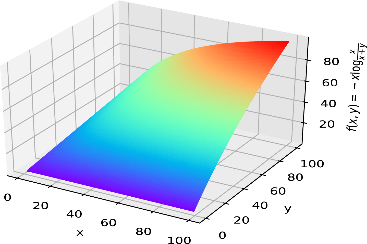
f(x,y)

Note that $q_{ij}^{(1)} \leq p_{ij}^{(1)}, q_{ij}^{(2)} \leq p_{ij}^{(2)} .$ Then $f (q_{ij}^{(1)}, q_{ij}^{(2)}) \leq f (p_{ij}^{(1)}, q_{ij}^{(2)}) \leq f (p_{ij}^{(1)}, p_{ij}^{(2)}) .$

Thus $H^{λ} (Q | d) \leq H^{λ} (P | d) .$

(2) ∀ i, j, denote $s_{ij}^{(1)} = | R_{P}^{λ_{1}} (o_{i}) \cap D_{j} |, s_{ij}^{(2)} = | R_{P}^{λ_{1}} (o_{i}) \cap (O - D_{j}) |;$ $t_{ij}^{(1)} = | R_{P}^{λ_{2}} (o_{i}) \cap D_{j} |, t_{ij}^{(2)} = | R_{P}^{λ_{2}} (o_{i}) \cap (O - D_{j}) | .$

By Proposition 2.5, we have $\forall i, R_{P}^{λ_{1}} (o_{i}) \subseteq R_{P}^{λ_{2}} (o_{i}) .$

Clearly, $0 \leq s_{ij}^{(1)} \leq t_{ij}^{(1)}, 0 \leq s_{ij}^{(2)} \leq t_{ij}^{(2)};$ $s_{ij}^{(1)} + s_{ij}^{(2)} = | R_{P}^{λ_{1}} (o_{i}) |, t_{ij}^{(1)} + t_{ij}^{(2)} = | R_{P}^{λ_{2}} (o_{i}) | .$

Then $\begin{matrix} H^{λ_{1}} (P | d) & = - \sum_{i = 1}^{n} \sum_{j = 1}^{r} \frac{| R_{P}^{λ_{1}} (o_{i}) \cap D_{j} |}{n} {log}_{2} \frac{| R_{P}^{λ_{1}} (o_{i}) \cap D_{j} |}{| R_{P}^{λ_{1}} (o_{i}) |} \\ = - \sum_{i = 1}^{n} \sum_{j = 1}^{r} \frac{s_{ij}^{(1)}}{n} {log}_{2} \frac{s_{ij}^{(1)}}{s_{ij}^{(1)} + s_{ij}^{(2)}} \\ ≜ \frac{1}{n} \sum_{i = 1}^{n} \sum_{j = 1}^{r} f (s_{ij}^{(1)}, s_{ij}^{(2)}) . \end{matrix}$ $\begin{matrix} H^{λ_{2}} (P | d) & = - \sum_{i = 1}^{n} \sum_{j = 1}^{r} \frac{| R_{P}^{λ_{2}} (o_{i}) \cap D_{j} |}{n} {log}_{2} \frac{| R_{P}^{λ_{2}} (o_{i}) \cap D_{j} |}{| R_{P}^{λ_{2}} (o_{i}) |} \\ = - \sum_{i = 1}^{n} \sum_{j = 1}^{r} \frac{t_{ij}^{(1)}}{n} {log}_{2} \frac{t_{ij}^{(1)}}{t_{ij}^{(1)} + t_{ij}^{(2)}} \\ ≜ \frac{1}{n} \sum_{i = 1}^{n} \sum_{j = 1}^{r} f (t_{ij}^{(1)}, t_{ij}^{(2)}) . \end{matrix}$

Note that $s_{ij}^{(1)} \leq t_{ij}^{(1)}, s_{ij}^{(2)} \leq t_{ij}^{(2)} .$ Then $f (s_{ij}^{(1)}, s_{ij}^{(2)}) \leq f (t_{ij}^{(1)}, s_{ij}^{(2)}) \leq f (t_{ij}^{(1)}, t_{ij}^{(2)}) .$

Thus $H^{λ_{1}} (P | d) \leq H^{λ_{2}} (P | d) .$ □

Definition 3.5. Suppose that (O, C ∪ {d}) is a gene decision space with P ⊆ C and λ ∈ [0, 1]. Then λ-joint information entropy of P and d is defined as $H^{λ} (P \cup d) = - \sum_{i = 1}^{n} \sum_{j = 1}^{r} \frac{| R_{P}^{λ} (o_{i}) \cap D_{j} |}{n} {log}_{2} \frac{| R_{P}^{λ} (o_{i}) \cap D_{j} |}{n}$ (3.3)

Proposition 3.6. Suppose that (O, C ∪ {d}) is a gene decision space with P ⊆ C and λ ∈ [0, 1]. Then

$H^{λ} (P | d) = H^{λ} (P \cup d) - H^{λ} (P)$ (3.4)

Proof. Note that {D₁, D₂ ⋯ , D_r} is a partition of O. Then ∀ i, $\sum_{j = 1}^{r} | R_{P}^{λ} (o_{i}) \cap D_{j} | = | R_{P}^{λ} (o_{i}) | .$ $\begin{matrix} H^{λ} (P | d) & = - \sum_{i = 1}^{n} \sum_{j = 1}^{r} \frac{| R_{P}^{λ} (o_{i}) \cap D_{j} |}{n} {log}_{2} \frac{| R_{P}^{λ} (o_{i}) \cap D_{j} |}{| R_{P}^{λ} (o_{i}) |} \\ = - \sum_{i = 1}^{n} \sum_{j = 1}^{r} \frac{| R_{P}^{λ} (o_{i}) \cap D_{j} |}{n} ({log}_{2} \frac{| R_{P}^{λ} (o_{i}) \cap D_{j} |}{n} \\ - {log}_{2} \frac{| R_{P}^{λ} (o_{i}) |}{n}) \end{matrix}$ $\begin{matrix} = - \sum_{i = 1}^{n} \sum_{j = 1}^{r} \frac{| R_{P}^{λ} (o_{i}) \cap D_{j} |}{n} {log}_{2} \frac{| R_{P}^{λ} (o_{i}) \cap D_{j} |}{n} + \\ \sum_{i = 1}^{n} \sum_{j = 1}^{r} \frac{| R_{P}^{λ} (o_{i}) \cap D_{j} |}{n} {log}_{2} \frac{| R_{P}^{λ} (o_{i}) |}{n} \\ = H^{λ} (P \cup d) + \sum_{i = 1}^{n} \frac{| R_{P}^{λ} (o_{i}) |}{n} {log}_{2} \frac{| R_{P}^{λ} (o_{i}) |}{n} \\ = H^{λ} (P \cup d) - H^{λ} (P) . \end{matrix}$ □

Theorem 3.7. Let (O, C ∪ {d}) be a gene decision space with P ⊆ C and λ ∈ [0, 1]. Then H^λ (P|d) ≥0.

Proof. By Definition 3.1, we have $H^{λ} (P) = - \sum_{i = 1}^{n} \frac{| R_{P}^{λ} (o_{i}) |}{n} {log}_{2} \frac{| R_{P}^{λ} (o_{i}) |}{n} .$

Note that {D₁, D₂ ⋯ , D_r} is a partition of O. Then ∀ i, $\sum_{j = 1}^{r} | R_{P}^{λ} (o_{i}) \cap D_{j} | = | R_{P}^{λ} (o_{i}) | .$

Then $H^{λ} (P) = - \sum_{i = 1}^{n} \frac{\sum_{j = 1}^{r} | R_{P}^{λ} (o_{i}) \cap D_{j} |}{n} {log}_{2} \frac{| R_{P}^{λ} (o_{i}) |}{n}$ $= - \sum_{i = 1}^{n} \sum_{j = 1}^{r} \frac{| R_{P}^{λ} (o_{i}) | \cap D_{j} |}{n} {log}_{2} \frac{| R_{P}^{λ} (o_{i}) |}{n} .$

By Definition 3.5, we have $H^{λ} (P \cup d) = - \sum_{i = 1}^{n} \sum_{j = 1}^{r} \frac{| R_{P}^{λ} (o_{i}) \cap D_{j} |}{n} {log}_{2} \frac{| R_{P}^{λ} (o_{i}) \cap D_{j} |}{n} .$

∀ i, j, $\log_{2} \frac{| R_{P}^{λ} (o_{i}) \cap D_{j} |}{n} \leq \log_{2} \frac{| R_{P}^{λ} (o_{i}) |}{n} .$

Then $H^{λ} (P) \leq H^{λ} (P \cup d) .$

By Proposition 3.6, $H^{λ} (P | d) = H^{λ} (P \cup d) - H^{λ} (P) .$

Hence H^λ (P|d) ≥0 .□

Lemma 3.8. Suppose that (O, C ∪ {d}) is a gene decision space with P ⊆ C and λ ∈ [0, 1]. If $R_{P}^{λ} \subseteq T_{d}$ , then ∀ o ∈ O, ∀ j, $R_{P}^{λ} (o) \cap D_{j} = {\begin{matrix} R_{P}^{λ} (o) & o \in D_{j} \\ \emptyset & o \notin D_{j} \end{matrix}$ (3.5)

Proof. If o ∈ D_j, then D_j = T_d (o). Since $R_{P}^{λ} \subseteq T_{d}$ , we have $R_{P}^{λ} (o) \subseteq T_{d} (o)$ . Thus $R_{P}^{λ} (o) \cap D_{j} = R_{P}^{λ} (o)$ .

If o ∉ D_j, then T_d (o)∩ D_j = ∅. Note that $R_{P}^{λ} \subseteq T_{d}$ . Then $R_{P}^{λ} (o) \subseteq T_{d} (o)$ . Thus $R_{P}^{λ} (o) \cap D_{j} = \emptyset$ . □

Lemma 3.9. Let (O, C ∪ {d}) be a gene decision space with P ⊆ C and λ ∈ [0, 1]. Suppose $R_{P}^{λ} \subseteq T_{d}$ . Then ∀ o ∈ O,

$\sum_{j = 1}^{r} \frac{| R_{P}^{λ} (o) \cap D_{j} |}{n} {log}_{2} \frac{| R_{P}^{λ} (o) \cap D_{j} |}{n}$

$= \frac{| R_{P}^{λ} (o) |}{n} {log}_{2} \frac{| R_{P}^{λ} (o) |}{n}$ .

Proof. Note that {D₁, D₂ ⋯ , D_r} is a partition of O. Then ∃ j^*, o ∈ D_{j
^*}.

Since $R_{P}^{λ} \subseteq T_{d}$ , by Lemma 3.8, we have $R_{P}^{λ} (o) \cap D_{j} = {\begin{matrix} R_{P}^{λ} (o) & j = j^{*} \\ \emptyset & j \neq j^{*} \end{matrix} .$

Thus

$\sum_{j = 1}^{r} \frac{| R_{P}^{λ} (o) \cap D_{j} |}{n} {log}_{2} \frac{| R_{P}^{λ} (o) \cap D_{j} |}{n}$

$= \frac{| R_{P}^{λ} (o) |}{n} {log}_{2} \frac{| R_{P}^{λ} (o) |}{n} .$ □

Theorem 3.10. Suppose that (O, C ∪ {d}) is a gene decision space with P ⊆ C and λ ∈ [0, 1]. Then the following conditions are equivalent:

(1) $R_{P}^{λ} \subseteq T_{d}$ ;

(2) H^λ (P∪ d) = H^λ (P) ;

(3) H^λ (P|d) =0.

Proof. (1) ⇒ (2). This holds by Lemma 3.9.

(2) ⇒ (1). Suppose H^λ (P ∪ d) = H^λ (P) .

Then $\begin{matrix} - \sum_{i = 1}^{n} \frac{| R_{P}^{λ} (o_{i}) |}{n} {log}_{2} \frac{| R_{P}^{λ} (o_{i}) |}{n} \\ = - \sum_{i = 1}^{n} \sum_{j = 1}^{r} \frac{| R_{P}^{λ} (o_{i}) \cap D_{j} |}{n} {log}_{2} \frac{| R_{P}^{λ} (o_{i}) \cap D_{j} |}{n} . \end{matrix}$

Note that {D₁, D₂ ⋯ , D_r} is a partition of O. Then ∀ i, $\sum_{j = 1}^{r} | R_{P}^{λ} (o_{i}) \cap D_{j} | = | R_{P}^{λ} (o_{i}) | .$

Then $\begin{matrix} - \sum_{i = 1}^{n} \sum_{j = 1}^{r} \frac{| R_{P}^{λ} (o_{i}) \cap D_{j} |}{n} {log}_{2} \frac{| R_{P}^{λ} (o_{i}) |}{n} \\ = - \sum_{i = 1}^{n} \sum_{j = 1}^{r} \frac{| R_{P}^{λ} (o_{i}) \cap D_{j} |}{n} {log}_{2} \frac{| R_{P}^{λ} (o_{i}) \cap D_{j} |}{n} . \end{matrix}$

So $\begin{matrix} \sum_{i = 1}^{n} \sum_{j = 1}^{r} \frac{| R_{P}^{λ} (o_{i}) \cap D_{j} |}{n} ({log}_{2} \frac{| R_{P}^{λ} (o_{i}) |}{n} - \\ {log}_{2} \frac{| R_{P}^{λ} (o_{i}) \cap D_{j} |}{n}) = 0 . \end{matrix}$

Thus $\sum_{i = 1}^{n} \sum_{j = 1}^{r} \frac{| R_{P}^{λ} (o_{i}) \cap D_{j} |}{n} {log}_{2} \frac{| R_{P}^{λ} (o_{i}) |}{| R_{P}^{λ} (o_{i}) \cap D_{j} |} = 0 .$

Suppose $R_{P}^{λ} ⊈ T_{d} .$ Then ∃ i^*, $R_{P}^{λ} (o_{i^{*}}) ⊈ T_{d} (o_{i^{*}}) .$ Denote T_d (o_{i
^*}) = D_{j
^*} .

We have $| R_{P}^{λ} (o_{i^{*}}) | > | R_{P}^{λ} (o_{i}) \cap D_{j^{*}} | .$

This follows that $\frac{| R_{P}^{λ} (o_{i^{*}}) \cap D_{j^{*}} |}{n} {log}_{2} \frac{| R_{P}^{λ} (o_{i^{*}}) |}{| R_{P}^{λ} (o_{i^{*}}) \cap D_{j^{*}} |} > 0 .$

Note that $\forall i, j, | R_{P}^{λ} (o_{i}) | \geq | R_{P}^{λ} (o_{i}) \cap D_{j} | .$ Then $\forall i, j, \frac{| R_{P}^{λ} (o_{i}) \cap D_{j} |}{n} {log}_{2} \frac{| R_{P}^{λ} (o_{i}) |}{| R_{P}^{λ} (o_{i}) \cap D_{j} |} \geq 0 .$

So $\sum_{i = 1}^{n} \sum_{j = 1}^{r} \frac{| R_{P}^{λ} (o_{i}) \cap D_{j} |}{n} {log}_{2} \frac{| R_{P}^{λ} (o_{i}) |}{| R_{P}^{λ} (o_{i}) \cap D_{j} |} > 0 .$ This is a contradiction.

Hence $R_{P}^{λ} \subseteq T_{d} .$

(2) ⇔ (3). This follows from Proposition 3.6.□

Theorem 3.11. Assume that (O, C ∪ {d}) is a gene decision space with λ ∈ [0, 1]. Then (O, C ∪ {d}) is λ-consistent ⇔ H^λ (C|d) =0 .

Proof. It follows from Theorems 2.9 and 3.10. □

4 Gene selection in a gene decision space

In this section, Gene selection in a gene decision space is investigated.

Definition 4.1. Let (O, C ∪ {d}) be a gene decision space with P ⊆ C and λ ∈ [0, 1]. Then P is referred to as a coordination subset of C to d, if H^λ (P|d) = H^λ (C|d).

The family of all coordination subsets of C to d is recorded as co_d (C).

Definition 4.2. Let (O, C ∪ {d}) be a gene decision space with P ⊆ C and λ ∈ [0, 1]. Then P is called a gene selection subset or reduct of C to d, if P ∈ co_d (C) and ∀ a ∈ P, P - {a} ∉ co_d (C).

The family of all gene selection subsets of C to d is recorded as red^d (C).

Definition 4.3. For a gene decision space (O, C ∪ {d}), given P ∈ red^d (C). The gene selection ratio RedR of P relative to C is defined as $RedR (P | C) = \frac{| C | - | P |}{| C |}$ (4.1)

Definition 4.4. Let (O, C ∪ {d}) be a gene decision space with P ⊆ C and λ ∈ [0, 1]. For any a ∈ P, inner-significance of the gene a for P relative to d is defined as ${sig}^{i} (a, P, d) = H^{λ} (P - {a} | d) - H^{λ} (P | d)$ (4.2)

Definition 4.5. Let (O, C ∪ {d}) be a gene decision space with P ⊆ C and λ ∈ [0, 1]. For any a ∈ C - P, outer-significance of the gene a for P relative to d is defined as ${sig}^{o} (a, P, d) = H^{λ} (P | d) - H^{λ} (P \cup {a} | d)$ (4.3)

We stipulate that $H^{λ} (\emptyset | d) = \max {H^{λ} ({c} | d) : c \in C}$ (4.4)

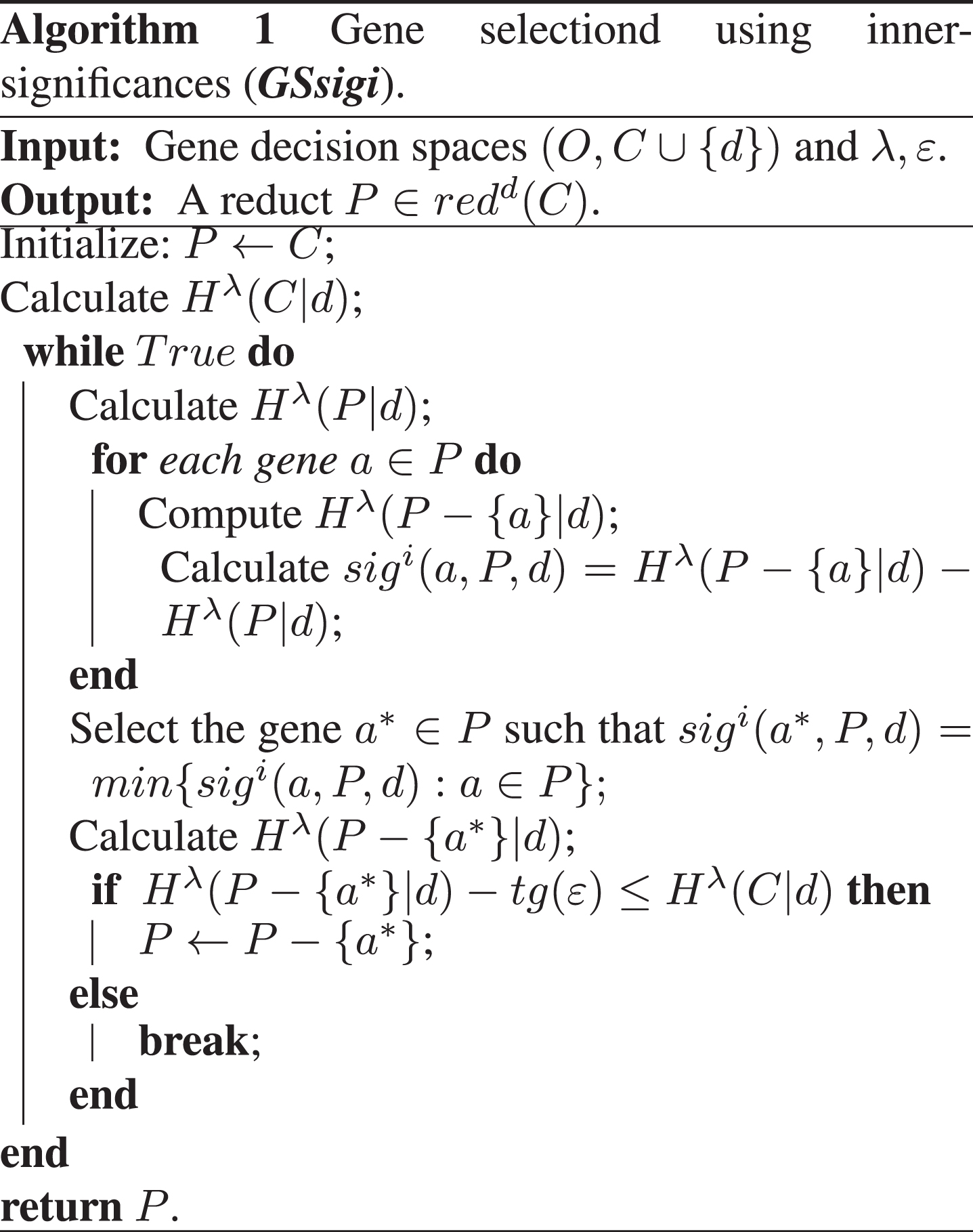
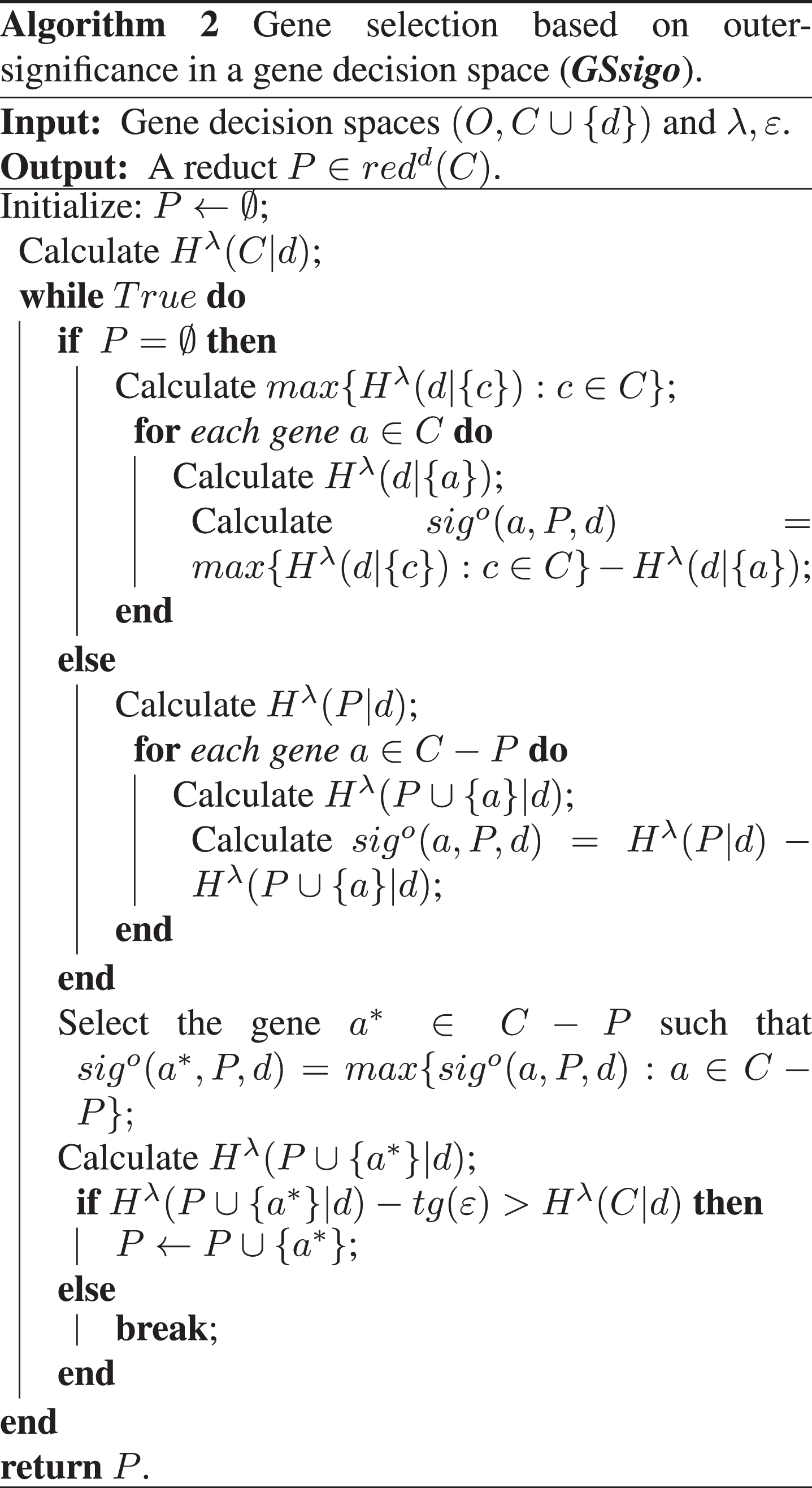
The computational complexity of an algorithm is commonly assessed using the time and space complexity to estimate its efficiency. The big oh notation is a commonly used to analyze the time and space complexities of algorithms.

In Algorithm “GSsigi", the basic execution time is determined by the ‘while’ loop in lines 3-16, while the ‘for’ in lines 5-8 runs one loop for each ‘while’. The total loops are equal to the product of the ‘while’ and ‘for’ loops. Assuming that the operation of calculating H^λ (P - {a} |d) is a basic operation, time complexity of ‘for’ is O (m). The execution times of the ‘while’ are determined by line 11, which respectively executes once and m times in the best and worst case. Therefore, time complexity of Algorithm “GSsigi" is respectively O (m) and O (m²) in the best and worst case. Assuming |P| = m_P, time complexity of Algorithm “GSsigi" is O (m_P (m - m_P)). In most cases, m_P ⪡ m, so time complexity of Algorithm “GSsigi" is approximately equal to O (m).

Algorithm “GSsigo" has a similar loop structure to Algorithm “GSsigi", so its time complexity is also O (m).

In this study, we introduce Fisher score [39, 51] to acquire preliminary subsets from gene spaces. The below briefly describes Fisher score.

Definition 4.6. In gene space (O, C), Fisher score f (c_j) of gene c_j ∈ C is calculated as $f (c_{j}) = \frac{\sum_{k = 1}^{K} n_{k} {(μ_{k}^{j} - μ^{j})}^{2}}{(\sum_{k = 1}^{K} n_{k} {(σ_{k}^{j})}^{2}) + τ}$ (4.5)

Formula (4.5) involves several variables, including the number of clusters, the ground truth vectors, the number of cells in each cluster, and the average value and standard deviation of the gene expression values within each cluster. A small value is added to prevent flow errors.

To select a subset of genes utilizing Fisher score, Algorithm 3 is presented, which takes the expected number of candidate genes as input and uses Fisher score to rank the genes. The time complexity of this algorithm is O (m), where m is gene number.

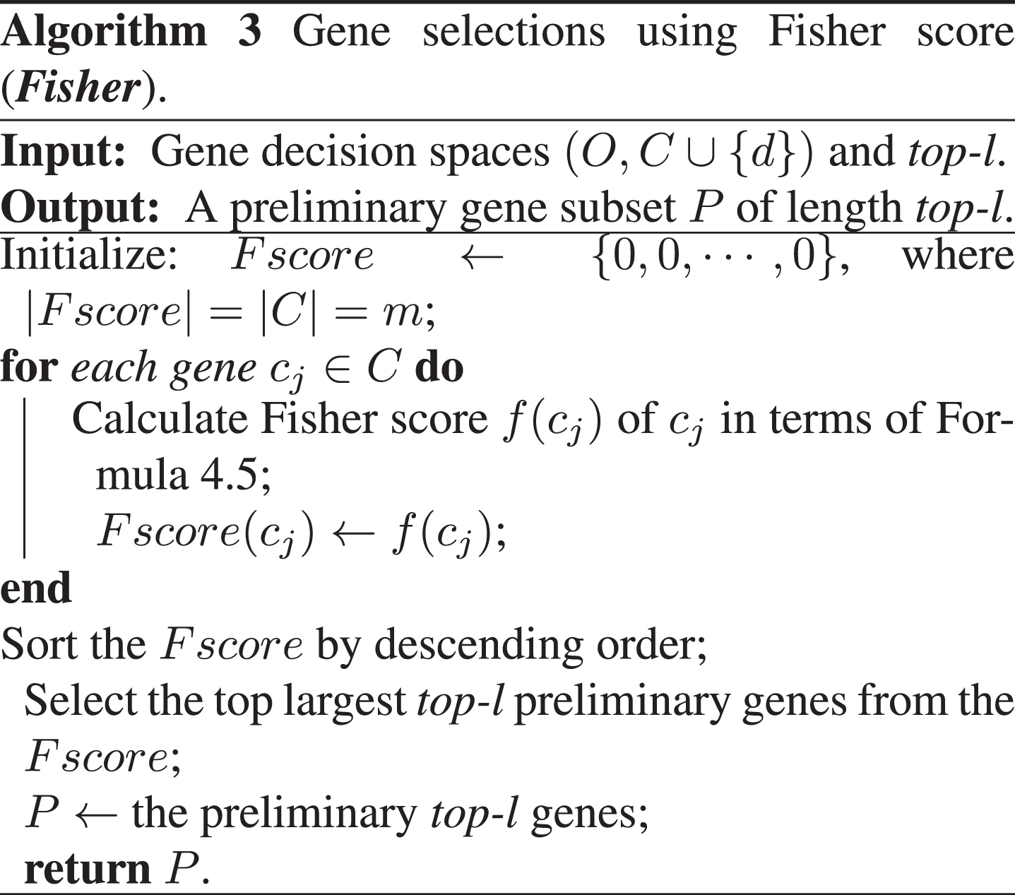
To ulteriorly lessen the time complexity of gene selection algorithms, Algorithm “Fisher" can be utilized to get a preliminary subset of genes, which is then used as input for Algorithms “GSsigi" or “GSsigo". As the preliminary subset is typically much smaller than the original set, the time complexity of the subsequent algorithms is greatly lessened. These modified algorithms are respectively referred to as “GSFsigi" and “GSFsigo".

Algorithm 4 Gene selections using Fisher score and inner-significances (GSFsigi).

Input: Gene decision spaces (O, C ∪ {d}), λ, ɛ and top-l.

Output: A reduct P ∈ red^d (C).

Implement Fisher to get

\bar{P} \subseteq C

by (O, C ∪ {d}) and top-l;

Implement GSsigi to acquire reduct

P \subseteq \bar{P}

(O, \bar{P} \cup {d})

;

return P

Algorithm 5 Gene selections using Fisher score and outer-significances (GSFsigo).

Input: Gene decision spaces (O, C ∪ {d}), λ, ɛ and top-l.

Output: A reduct P ∈ red^d (C).

Execute Fisher to search

\bar{P} \subseteq C

by (O, C ∪ {d}) and top-l;

Execute GSsigo to find reduct

P \subseteq \bar{P}

(O, \bar{P} \cup {d})

;

return P

In Algorithm “GSFsigi", time complexity of “Fisher" is O (m). Supposing that the cardinality of the $\bar{P}$ obtained by “Fisher" is equal to $m_{\bar{P}}$ , namely $| \bar{P} | = m_{\bar{P}}$ . Then time complexity of “GSsigi" is $O (m_{\bar{P}})$ necessarily. Commonly $m_{\bar{P}} ⪡ m$ , thus $O (m_{\bar{P}})$ lessens dramatically. Similarly, time complexity of “GSsigo" is also lessened greatly.

5 Application to classifications for gene data

Gene data have high-level noises and high dimensions due to technical and sampling reasons. Thus, it not easy to accurately classify different cells. To eliminate the noises and decrease the dimensions, the section applies the presented gene selection algorithms GSsigi and GSsigi to gene expression data classifications. By means of gene selection, we can select suitable genes for gene expression data and decrease the dimension, time complexity and space complexity of classifications will be improved greatly.

In this section, several publicly available gene expression datasets are utilized to perform classification tasks. Two classifiers KNN (K-Nearest Neighbor) and CART (a decision tree) are employed as classification methods. We designed the following numerical experiments. The below experiments will execute the above gene selections in gene decision spaces to select suitable genes related to classifications, then respectively perform two classifiers to perform classification tasks. The performance of gene selection algorithms is evaluated using the accuracy of classification (ACC). To mitigate the impact of randomness, each gene expression dataset is partitioned into 10 folds, with one fold serving as the test subset and the remaining folds as training subsets. The ACC of the dataset with respect to the classifier is determined by calculating the average ACC of the 10 test subsets for both KNN and CART classifiers.

5.1 Data sets and data normalization

The performance of the proposed algorithms is evaluated using several publicly available gene expression datasets with varying orders of magnitude, as shown in Table 1. The numbers of cells and genes are represented by # cells and # genes, while # classes indicates the number of ground truths. The datasets are categorized into three types based on gene number, namely low, middle, and high, as indicated in the “Dimension” of Table 1. This is utilized to determine the number of preliminary genes (# preliminary genes). For the datasets of type “low", # preliminary genes is set as gene number. For the datasets of type “middle" and “high", # preliminary genes is respectively set as 100 and 300. The # preliminary genes is just top-l in Algorithms 3–5. In Table 1, the “source" provides the addresses to search datasets. Among, “address1", “address2" and “address3" denote “http://archive.ics.uci.edu/ml/index.php", “http://csse.szu.edu.cn/staff/zhuzx/Datasets.html", and “http://featureselection.asu.edu/datasets.php", respectively.

Table 1
Gene expression datasets

Name #cells #genes #classes Dimension #preliminary Source References

genes

Glass 214 9 6 low 9 address1 Rao et al. [30]

Ionosphere 351 34 2 low 34 address1 Wang et al. [48]

Sonar 208 60 2 low 60 address1 Souza et al. [34]

Colon 62 2000 2 middle 100 address2 Dong et al. [12]

Lymphoma 66 4026 3 middle 100 address2 Li et al. [25]

SRBCT 83 2308 4 middle 100 address2 Dong et al. [12]

CLL_SUB 111 11340 3 high 300 address3 Wu et al. [47]

Lung 203 12600 5 high 300 address2 Shukla et al. [37]

Ovarian 253 15154 2 high 300 address2 Seijo-Pardo et al. [32]

SMK_CAN 187 19993 2 high 300 address3 Wu et al. [47]

Name	#cells	#genes	#classes	Dimension	#preliminary	Source	References
Glass	214	9	6	low	9	address1	Rao et al. [30]
Ionosphere	351	34	2	low	34	address1	Wang et al. [48]
Sonar	208	60	2	low	60	address1	Souza et al. [34]
Colon	62	2000	2	middle	100	address2	Dong et al. [12]
Lymphoma	66	4026	3	middle	100	address2	Li et al. [25]
SRBCT	83	2308	4	middle	100	address2	Dong et al. [12]
CLL_SUB	111	11340	3	high	300	address3	Wu et al. [47]
Lung	203	12600	5	high	300	address2	Shukla et al. [37]
Ovarian	253	15154	2	high	300	address2	Seijo-Pardo et al. [32]
SMK_CAN	187	19993	2	high	300	address3	Wu et al. [47]

To decrease too much influence of large values versus small values, the following definition is employed to standardize each element in the gene expression dataset [54]. In (O, C ∪ {d}), c_j (o_i) can be standardized using the ensuing formula.

$\tilde{c_{j} (o_{i})} = \frac{c_{j} (o_{i}) - c_{j}^{min}}{c_{j}^{max} - c_{j}^{min}}$ (5.1)

where $c_{j}^{min} = \min {c_{j} (x_{i}) : i = 1, 2, \dots, n}$ $c_{j}^{max} = \max {c_{j} (x_{i}) : i = 1, 2, \dots, n}$

It is evident that Formula (5.1) has the ability to standardize c_j (o_i) to [0, 1]. This process can effectively reduce the variations among genes in (O, C ∪ {d}).

5.2 Experiment flow and setup

The experiments commence by normalizing the data in gene decision space as described in subsection 5.1. Subsequently, the presented algorithms, PCA, tSNE, and two state-of-the-art gene selection algorithms, FMIFRFS and DNEAR, are implemented in the normalized gene decision space to obtain several gene decision subspaces. Finally, classification methods are executed on the normalized gene space and several obtained gene subspaces to calculate several evaluation metrics, including gene number, RedR and ACC. Figure 3 provides a detailed illustration of experiment process.

Fig. 3

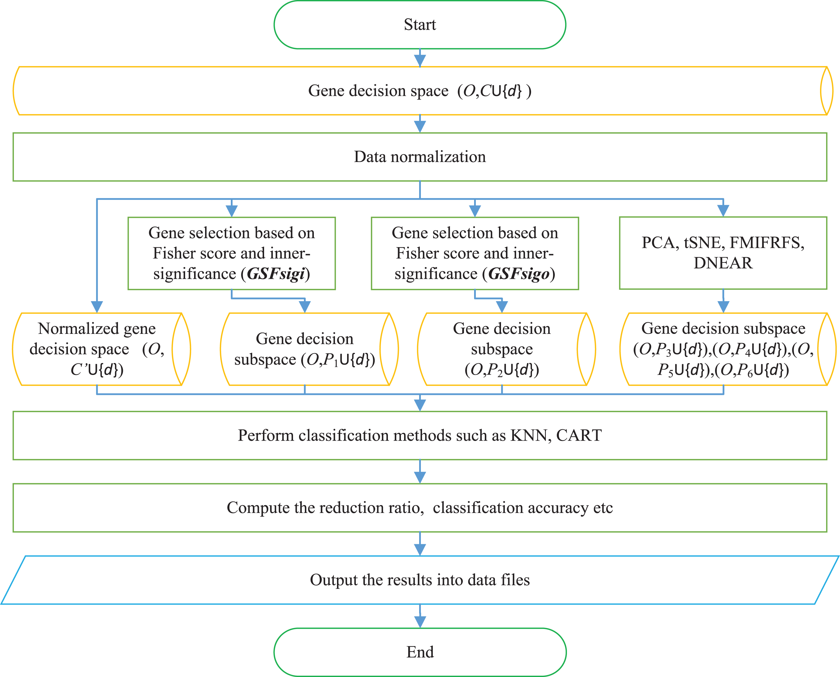
Experimental flow.

To substantiate the credibility of GSFsigi and GSFsigo, the subsequent algorithms are utilized to conduct a comparative analysis.

Two prevalent techniques for dimensionality reduction

PCA

tSNE

Two state-of-the-art gene selection algorithms

FMIFRFS

DNEAR

In order to ensure a just comparison and efficient time complexity, the FMIFRFS algorithm initially employs Fisher method to derive a preliminary set of genes based on top-l, then performs the FMIFRFS on the obtained gene subset. The parameters top-l used in the FMIFRFS, λ and top-l used in the DNEAR are setup as the same values as those of the proposed GSFsigi and GSFsigo.

The first step of the experiment involves normalizing each gene within 0 to 1, followed by the implementation of several algorithms to obtain multiple gene decision subspaces. The effectiveness of two gene selection algorithms is then evaluated by employing two frequently used classifiers, KNN and CART, in original gene space and the resulting subspaces. In order to compare the performance of these algorithms, several metrics including gene number, RedR and ACC are considered.

The parameter preferences of the competing methods and two classifiers are outlined in Table 2. The λ parameter acts as a threshold in the entropy measure, while the ɛ parameter is employed to obtain an ɛ-approximate. The top-l parameter represents the anticipated number of preliminary genes utilized in Fisher, GSFsigi, GSFsigo, IFMIFRFS, and DNEAR. The NumDimensions parameter refers to the output dimension used in tSNE, whereas the NumNeighbors parameter denotes the number of nearest neighbors utilized in KNN.

Table 2

Parameter values

Type	Algorithm	Parameter	Value
Gene selection	GSFsigi, GSFsigo	λ	0.3
/dimension reduction		ɛ	0.1
		top-l	“#preliminary genes” in Table 1
	Fisher	top-l	“#preliminary genes” in Table 1
	PCA	all parameters	default
	tSNE	NumDimensions	min(\|O\|, \|C\|)
	IFMIFRFS	top-l	“#preliminary genes" in Table 1
	DNEAR	δ	0.3
		top-l	“#preliminary genes” in Table
Classifier	KNN	NumNeighbors	5
	CART	all parameters	default

The GSFsigi, GSFsigo, IFMIFRFS and DNEAR have been developed and implemented in the Matlab platform, whereas the PCA, tSNE, KNN and CART employ the built-in functions in Matlab.

5.3 Comparisons of experimental results

To effectively demonstrate the effectiveness of the proposed algorithms GSFsigi and GSFsigo, the experiments have been partitioned into three distinct parts. Firstly, a comparison is made between the GSFsigi and GSFsigo, raw data, and Fisher. Secondly, the GSFsigi and GSFsigo are compared with two frequently used dimensionality reduction methods, PCA and tSNE. Lastly, the proposed algorithms are compared with two state-of-the-art gene selection methods, FMIFRFS and DNEAR. Various evaluation metrics, including gene number, RedR and ACC, are calculated to evaluate the performances of algorithms. The KNN and CART classifiers are employed to calculate ACC.

5.3.1 Comparisons with raw data and Fisher

The experiment first compares the proposed gene selection algorithms with raw data and Fisher. The number of genes and RedR are shown in Table 3, and the ACC metrics obtained by two classifiers are manifested in Table 4.

Table 3
Gene number chosen by GSFsigi, GSFsigo, raw data and Fisher

Datasets Number of genes RedR(%)

Raw Fisher GSFsigi GSFsigo Raw Fisher GSFsigi GSFsigo

Glass 9 9 8 7 0 0 11.11 22.22

Ionosphere 34 34 27 25 0 0 20.59 26.47

Sonar 60 60 29 27 0 0 51.67 55.00

Colon 2000 100 17 12 0 95.00 99.15 99.40

Lymphoma 4026 100 7 4 0 97.52 99.83 99.90

SRBCT 2308 100 14 7 0 95.67 99.39 99.70

CLL_SUB 11340 300 37 37 0 97.35 99.67 99.67

Lung 12600 300 20 21 0 97.62 99.84 99.83

Ovarian 15154 300 14 8 0 98.02 99.91 99.95

SMK_CAN 19993 300 32 17 0 98.50 99.84 99.91

Datasets	Number of genes		RedR(%)
Glass	9	9	8	7	0	11.11	22.22
Ionosphere	34	34	27	25	0	20.59	26.47
Sonar	60	60	29	27	0	51.67	55.00
Colon	2000	100	17	12	95.00	99.15	99.40
Lymphoma	4026	100	7	4	97.52	99.83	99.90
SRBCT	2308	100	14	7	95.67	99.39	99.70
CLL_SUB	11340	300	37	37	97.35	99.67	99.67
Lung	12600	300	20	21	97.62	99.84	99.83
Ovarian	15154	300	14	8	98.02	99.91	99.95
SMK_CAN	19993	300	32	17	98.50	99.84	99.91

Table 4

ACC obtained by GSFsigi, GSFsigo, raw data and Fisher

Datasets	KNN				CART
	Raw	Fisher	GSFsigi	GSFsigo	Raw	Fisher	GSFsigi	GSFsigo
Glass	66.3853	66.3853	65	66.4069✓	67.3377	67.7922	69.2424✓	65.9307
Ionosphere	89.4683	89.4683	89.4762✓	89.4683	88.3175	87.4603	90.5873	90.8889✓
Sonar	80.7381	80.7381	81.7143	83.1190✓	73.6429✓	72.6429	73.0476	72.1667
Colon	74.5238	83.8095	86.9048✓	86.9048✓	79.0476	80.4762	83.5714✓	80.4762
Lymphoma	98.5714	100✓	98.5714	100✓	90.9524	89.2857	94.0476	95✓
SRBCT	81.8056	100✓	92.6389	96.3889	88.1944	89.4444	73.3333	90.4167✓
CLL_SUB	59.3939	58.4091	64.7727✓	57.5000	64.9242✓	61.1364	48.4848	50.3788
Lung	89.6429	93.5952	95.0476✓	94.5476	88.7381	93.1667✓	85.3333	83.2857
Ovarian	90.1385	97.2462	98.4154	99.2154✓	98.0308	98.4154	96.4308	98.8154✓
SMK_CAN	66.7836	66.2865	64.6491	74.2398✓	58.1871	64.7661	57.1345	72.1930✓

From Table 3, it is evident that the GSFsigi and GSFsigo is slightly reduced in comparison to the raw data and Fisher for the datasets categorized as "low". However, this reduction is significantly greater for datasets classified as "middle" and "high". This is because the number of preliminary genes for type “low" datasets is set as the number of original genes, while type “middle" and “high" datasets respectively are set as 100 and 300 in Subsection 5.1. The RedR metrics of GSFsigi and GSFsigo are significatly greater than those of raw data and Fisher. The datasets categorized as “middle" and “high" exhibit GSFsigi and GSFsigo exceed 99% in terms of RedR. This indicates a remarkable capacity for dimensionality reduction. We can also see that the gene number and RedR of GSFsigo are better than those of GSFsigi. This indicates that GSFsigo is superior to GSFsigi in terms of RedR and gene number.

Table 4 displays the performance of four algorithms, with the mark ’✓’ indicating the highest accuracy (ACC) achieved. The findings indicate that the proposed GSFsigi or GSFsigo outperforms raw data and Fisher in terms of ACC under the KNN and CART classifiers. Specifically, GSFsigi and GSFsigo achieve the highest accuracy in 9 and 7 out of 10 datasets, respectively. Furthermore, the comparison between GSFsigi and GSFsigo reveals that the latter achieves a larger number of highest accuracies, indicating its superiority over GSFsigi in terms of accuracy.

To sum up, it is evident that the proposed GSFsigo demonstrates a higher level of superiority than both the raw data and Fisher in relation to the gene number, RedR and ACC. Likewise, the GSFsigi exhibits a superior level of performance in comparison to the raw data with regards to the gene number, RedR and ACC. Additionally, the GSFsigo clearly outperforms the GSFsigi in terms of the gene number, RedR and ACC.

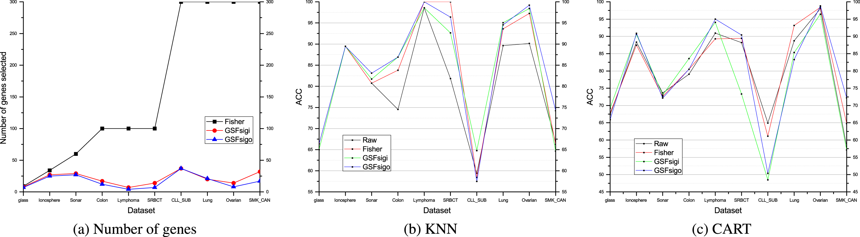
To provide a clear and intuitive representation of the efficacy of various algorithms, Fig. 4presents a detailed comparison of the GSFsigi, GSFsigo, raw data, and Fisher with respect to both gene number and ACC.

Fig. 4

Comparisons of GSFsigi, GSFsigo, raw data and Fisher.

Figure 4(a) displays the gene number, while ACC metrics for KNN and CART classifiers are illustrated in Fig. 4(b) and (c), respectively.

In all datasets, it is evident from Fig. 4(a) that both GSFsigi and GSFsigo outperform Fisher in terms of the gene number. Moreover, GSFsigi is comparable to GSFsigo in most datasets.

Figure 4(b) illustrates that the GSFsigo outperforms the raw data in most datasets, with the exception of “Glass", “Ionosphere" and “CLL_SUB". Similarly, the GSFsigi exhibits superior performance to the raw data in most datasets, except for “Glass", “Ionosphere", “Lymphoma" and “SMK_CAN". Notably, the GSFsigo surpasses the Fisher method in the datasets “Glass", “Sonar", “Colon", “Lung", “Ovarian" and “SMK_CAN". Additionally, the GSFsigi demonstrates notable superiority to the Fisher method in the datasets “Sonar", “Colon",“CLL_SUB", “Lung", and “Ovarian". Therefore, it can be concluded from Fig. 4(b) that the GSFsigo and GSFsigi exhibit superior performance to the raw data and Fisher method in at least half of the datasets.

According to Fig. 4(c), the GSFsigo outperforms the raw data in most datasets, with the exception of “Glass", “Sonar", “CLL_SUB" and“Lung". Additionally, the GSFsigi shows notable superiority to the raw data in “Glass", “Ionosphere", “Colon", and “Lymphoma". Furthermore, the GSFsigo surpasses the Fisher in “Ionosphere", “Lymphoma", “SRBCT" and “SMK_CAN", whereas the GSFsigi outperforms the Fisher in “Glass", “Ionosphere", “Sonar", “Colon" and “Lymphoma".

The evidence provided in Fig. 4(a), (b), and (c) leads to the conclusion that GSFsigi and GSFsigo exhibit notable superiority over the raw data and Fisher with regard to the gene number and and ACC.

5.3.2 Comparisons with PCA and tSNE

In the second phase of the study, the efficacy of the GSFsigi and GSFsigo is evaluated by comparing them with two widely employed dimensionality reduction techniques, namely PCA and tSNE. The tabulated data in Table 5 illustrates the obtained gene number and RedR. Additionally, Table 6 presents ACC metrics acquired by two classifiers.

Table 5
Gene number and RedR of GSFsigi, GSFsigo, PCA and tSNE

Datasets Number of genes RedR(%)

PCA tSNE GSFsigi GSFsigo PCA tSNE GSFsigi GSFsigo

Glass 9 9 8 7 0 0 11.11 22.22

Ionosphere 34 34 27 25 0 0 20.59 26.47

Sonar 60 60 29 27 0 0 51.67 55.00

Colon 61 62 17 12 96.95 96.90 99.15 99.40

Lymphoma 65 66 7 4 98.39 98.36 99.83 99.90

SRBCT 82 83 14 7 96.45 96.40 99.39 99.70

CLL_SUB 110 111 37 37 99.03 99.02 99.67 99.67

Lung 202 203 20 21 98.40 98.39 99.84 99.83

Ovarian 252 253 14 8 98.34 98.33 99.91 99.95

SMK_CAN 186 187 32 17 99.07 99.06 99.84 99.91

Table 6

ACC obtained by GSFsigi, GSFsigo, PCA and tSNE

Datasets	KNN				CART
	PCA	tSNE	GSFsigi	GSFsigo	PCA	tSNE	GSFsigi	GSFsigo
Glass	66.7965	64.9567	65	66.4069✓	63.9827	63.5714	69.2424✓	65.9307
Ionosphere	84.8810	86.8730	89.4762✓	89.4683	90.3095	87.4524	90.5873	90.8889✓
Sonar	82.7143	82.7143	81.7143	83.1190✓	71.1190	82.2381✓	73.0476	72.1667
Colon	77.6190	77.6190	86.9048✓	86.9048✓	61.4286	69.5238	83.5714✓	80.4762
Lymphoma	100✓	100✓	98.5714	100✓	92.6190	96.9048✓	94.0476	95
SRBCT	79.3056	83.3333	92.6389	96.3889✓	80.6944	79.3056	73.3333	90.4167✓
CLL_SUB	57.7273	44.8485	64.7727✓	57.5000	55✓	41.2879	48.4848	50.3788
Lung	89.5952	90.0714	95.0476✓	94.5476	85.2381	92.5238✓	85.3333	83.2857
Ovarian	93.3231	92.1231	98.4154	99.2154✓	81.9538	90.9077	96.4308	98.8154✓
SMK_CAN	67.8947	49.8830	64.6491	74.2398✓	62.1053	52.9240	57.1345	72.1930✓

Table 5 illustrates that the GSFsigi and GSFsigo approaches yield a lower gene number compared to PCA and tSNE for all datasets, particularly for datasets categorized as “middle" and “high". Additionally, the RedR values obtained by the GSFsigi and GSFsigo are higher than those obtained by PCA and tSNE. This demonstrates that the proposed GSFsigi and GSFsigo exhibit excellent reduction performance and are superior to PCA and tSNE with respect to gene number and RedR. Furthermore, a comparison between GSFsigi and GSFsigo reveals that the latter is superior, as RedR values of GSFsigo are superior to those of GSFsigi for all datasets.

The utilization of an ’✓’ mark in Table 6 indicates the highest accuracy among four algorithms. The results presented in Table 6 demonstrate that, when utilizing KNN and CART classifiers, the GSFsigi or GSFsigo algorithms achieve the highest accuracy respectively in 10 and 6 of 10 datasets. This observation highlights the superior performance of GSFsigi and GSFsigo over tSNE and PCA concerning accuracy under two classifiers.

To conclude, it is apparent that GSFsigi and GSFsigo exhibit superior performance compared to tSNE and PCA with respect to the gene number, RedR and ACC.

Based on the data presented in Tables 3–6, it can be inferred that GSFsigi and GSFsigo algorithms outperform the other methods, such as raw data, Fisher, tSNE, and PCA, in terms of gene number, RedR and ACC. This conclusion is either evident or comparatively evident. It can be deduced from this evidence that GSFsigi and GSFsigo algorithms are the most effective in these methods.

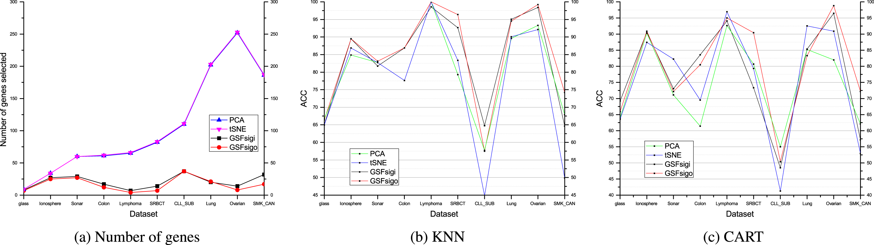
In order to provide a clear understanding of the effectiveness of multiple algorithms, Fig. 5 presents a detailed comparison of the GSFsigi, GSFsigo, PCA and tSNE, with respect to the gene number and two ACC metrics using KNN and CART. The purpose of this illustration is to intuitively showcase the differences in performance among these algorithms.

Fig. 5

Comparisons of GSFsigi, GSFsigo, PCA and tSNE.

The information presented in Fig. 5 can be divided into three parts: the gene number (Fig. 4(a)), and the ACC metrics for KNN and CART classifiers (Fig. 5(b) and (c), respectively).

The results in Fig. 5(a) indicate that GSFsigi and GSFsigo perform significantly better than PCA and tSNE in terms of gene number across all datasets. Furthermore, PCA and tSNE exhibit similar performance across all datasets, while GSFsigi and GSFsigo demonstrate comparable performance in most datasets.

Figure 5(b) illustrates that the GSFsigo clearly outperforms the PCA in most datasets except “Lymphoma" (equal) and “CLL_SUB" (approximately equal). Likewise, GSFsigi is evidently better than PCA in most datasets, except for “Glass", “Sonar", “Lymphoma" and “SMK_CAN". Furthermore, GSFsigo is significantly superior to tSNE in most datasets, except for “Lymphoma" (equal), while GSFsigi notably outperforms tSNE in most datasets, except for “Sonar" and “Lymphoma". To sum up, It can be seen from Fig. 5(b) that GSFsigo and GSFsigi exhibit superior performance compared to PCA and tSNE in most datasets.

Figure 5(c) depicts that the GSFsigo is significantly better than the PCA in most datasets, except for “CLL_SUB" and“Lung". Similarly, GSFsigi notably outperforms PCA in most datasets, except for “SRBCT", “CLL_SUB" and “SMK_CAN". Furthermore, GSFsigo exhibit significant superior performance compared to tSNE in most datasets except “Sonar", “Lymphoma" and “Lung", whereas GSFsigi markedly outperforms tSNE in most datasets, except for “Sonar", “Lymphoma", “SRBCT" and “Lung". Overall, Fig. 5(c) demonstrates that GSFsigo and GSFsigi algorithms exhibit superior performance compared to PCA and tSNE algorithms in most datasets.

We can conclude from Fig. 5(a), (b) and (c) that GSFsigi and GSFsigo obviously outperform PCA and tSNE with respect to gene number and ACC.

5.3.3 Comparisons with FMIFRFS and DNEAR

The third part of the experiment compares the proposed gene selection algorithms with two state-of-the-art gene selection algorithms, FMIFRFS and DNEAR. The tabulated data in Table 7 illustrates the obtained gene number and RedR, while Table 8 provides ACC metrics acquired by two classifiers.

Table 7
Gene number of GSFsigi, GSFsigo, FMIFRFS and DNEAR

Datasets Number of genes RedR(%)

FMIFRFS DNEAR GSFsigi GSFsigo FMIFRFS DNEAR GSFsigi GSFsigo

Glass 8 4 8 7 11.11 55.56 11.11 22.22

Ionosphere 1 32 27 25 97.06 5.88 20.59 26.47

Sonar 59 20 29 27 1.67 66.67 51.67 55.00

Colon 74 10 17 12 96.30 99.50 99.15 99.40

Lymphoma 90 11 7 4 97.76 99.73 99.83 99.90

SRBCT 99 11 14 7 95.71 99.52 99.39 99.70

CLL_SUB 84 12 37 37 99.26 99.89 99.67 99.67

Lung 299 4 20 21 97.63 99.97 99.84 99.83

Ovarian 171 19 14 8 98.87 99.87 99.91 99.95

SMK_CAN 225 12 32 17 98.87 99.94 99.84 99.91

Datasets	Number of genes		RedR(%)
Glass	8	4	8	7	11.11	55.56	11.11	22.22
Ionosphere	1	32	27	25	97.06	5.88	20.59	26.47
Sonar	59	20	29	27	1.67	66.67	51.67	55.00
Colon	74	10	17	12	96.30	99.50	99.15	99.40
Lymphoma	90	11	7	4	97.76	99.73	99.83	99.90
SRBCT	99	11	14	7	95.71	99.52	99.39	99.70
CLL_SUB	84	12	37	37	99.26	99.89	99.67	99.67
Lung	299	4	20	21	97.63	99.97	99.84	99.83
Ovarian	171	19	14	8	98.87	99.87	99.91	99.95
SMK_CAN	225	12	32	17	98.87	99.94	99.84	99.91

Table 8

ACC obtained by GSFsigi, GSFsigo, FMIFRFS and DNEAR

Datasets	KNN				CART
	FMIFRFS	DNEAR	GSFsigi	GSFsigo	FMIFRFS	DNEAR	GSFsigi	GSFsigo
Glass	65.3463	61.6450	65	66.4069✓	62.5758	67.7706	69.2424✓	65.9307
Ionosphere	78.6667	84.3333	89.4762✓	89.4683	78.0714	89.7302	90.5873	90.8889✓
Sonar	81.8095	80.1429	81.7143	83.1190✓	73.5238✓	61	73.0476	72.1667
Colon	86.9048✓	79.0476	86.9048✓	86.9048✓	75.9524	75.4762	83.5714✓	80.4762
Lymphoma	100✓	94.0476	98.5714	100✓	94.0476	86.9048	94.0476	95✓
SRBCT	100✓	72.5000	92.6389	96.3889	85	68.4722	73.3333	90.4167✓
CLL_SUB	60.3030	56.6667	64.7727✓	57.5000	55.7576✓	55.0758	48.4848	50.3788
Lung	95.0952✓	70.4524	95.0476	94.5476	89.6667✓	64.0476	85.3333	83.2857
Ovarian	98	98.4154	98.4154	99.2154✓	98.0154	96.4615	96.4308	98.8154✓
SMK_CAN	70.6433	63.0409	64.6491	74.2398✓	58.8304	53.9181	57.1345	72.1930✓

From Table 7, we can see that gene number obtained by GSFsigi and GSFsigo are far smaller than those obtained by FMIFRFS for most datasets except “Ionosphere". This signifies that the GSFsigi and GSFsigo are better than FMIFRFS with respect to the gene number and RedR. Compared to DNEAR, gene number obtained by the GSFsigi and GSFsigo are lower than those obtained by the DNEAR in 3 and 4 of 10 datasets, respectively. This indicates that GSFsigi and GSFsigo are not superior to the DNEAR in terms of gene number and RedR.

According to Table 8, in 10 datasets, GSFsigi or GSFsigo algorithms achieve the highest ACC under KNN and CART classifiers in 8 and 7 datasets, respectively. Likewise, FMIFRFS achieve the highest ACC in 4 and 3 datasets, whereas DNEAR does not obtain the largest ACC in all dataset. This reveals that GSFsigi and GSFsigo outperform FMIFRFS and DNEAR with regards to ACC.

By comparing Tables 8, we can observe that GSFsigi and GSFsigo are not superior to DNEAR in terms of gene number and RedR, but GSFsigi and GSFsigo are superior to DNEAR with respect to ACC. Therefore, the GSFsigi and GSFsigo are comparable to the DNEAR. Commonly, it is more preferable to obtain a high ACC than a high gene selection ratio. Namely, the GSFsigi and GSFsigo are comparatively superior to the DNEAR.

To sum up, both GSFsigi and GSFsigo are superior to FMIFRFS with respect to gene number, RedR and ACC for most datasets, and are better than DNEAR for all datasets under both KNN and CART classifiers.

Based on the data presented in Tables 3 –8, it can be inferred that GSFsigo outperforms the other algorithms, namely the raw data, Fisher, tSNE, PCA, FMIFRFS, and DNEAR. Similarly, GSFsigi is superior to the raw data, Fisher, tSNE, PCA, and DNEAR, but inferior to FMIFRFS.

To provide a clear and intuitive representation of the efficacy of various algorithms, Fig. 6 presents a comprehensive comparison of GSFsigi, GSFsigo, FMIFRFS and DNEAR with respect to gene number and ACC.

Fig. 6

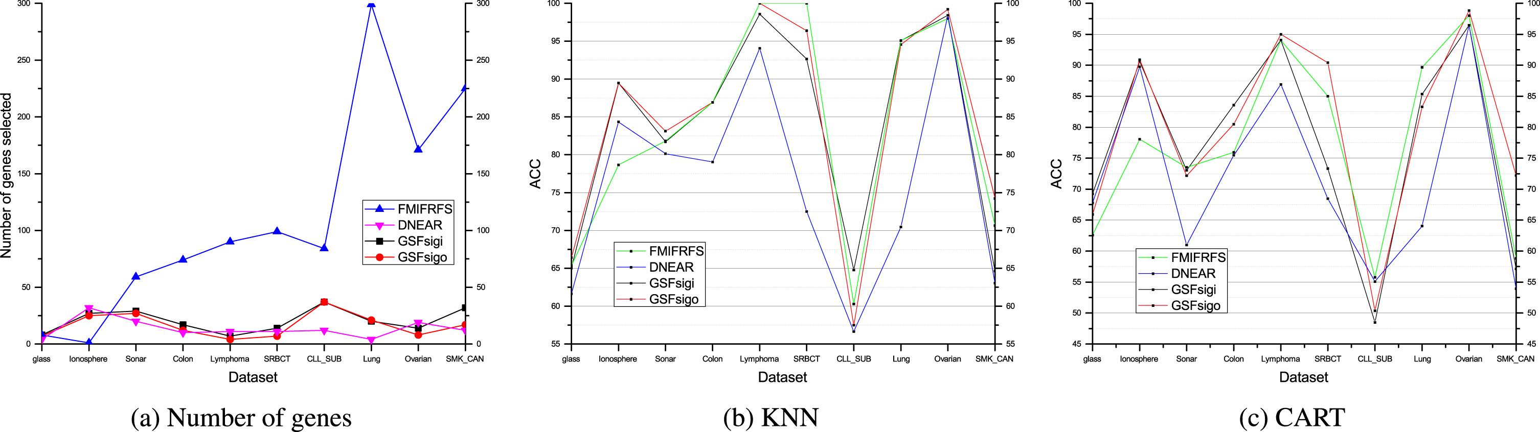
Comparisons of GSFsigi, GSFsigo, FMIFRFS and DNEAR.

Figure 6 can be divided into three parts: the gene number (Fig. 6(a)), and two ACC for KNN and CART classifiers (Fig. 6(b) and (c), respectively).

It can be seen from Fig. 6(a) that GSFsigi, GSFsigo and DNEAR are obviously superior to the FMIFRFS in terms of gene number in most datasets except “Ionosphere"; the GSFsigi, GSFsigo and DNEAR is approximate in most datasets.

Figure 6(b) illustrates that the GSFsigi and GSFsigo significantly outperform the DNEAR in all datasets; the GSFsigo is significantly superior to the FMIFRFS in most datasets except “SRBCT", “CLL_SUB" and “Lung”; the GSFsigi is better than FMIFRFS in the datasets “Ionosphere”, “Colon”, “CLL_SUB” and “Ovarian". To summarize, Fig. 6(b) depicts that the GSFsigo overtly outperforms the FMIFRFS and DNEAR, and the GSFsigi is superior to the DNEAR but inferior to the FMIFRFS.

Figure 6(c) depicts that the GSFsigo significantly outperforms the DNEAR in most datasets except “Glass" and “CLL_SUB"; the GSFsigo is markedly superior to the FMIFRFS in most datasets except “Sonar", “CLL_SUB" and “Lung"; the GSFsigi is clearly better than the DNEAR in most datasets except “CLL_SUB" and Ovarian (approximately equal); the GSFsigi is obviously superior to the FMIFRFS in the datasets “Glass", “Ionosphere" and “Colon". To summarize, Fig. 6(c) also illustrate that the GSFsigo overtly outperforms the FMIFRFS and DNEAR, and the GSFsigi is superior to the DNEAR but inferior to the FMIFRFS.

We can conclude from Figs. 4 –6 that GSFsigo is obviously better than the other approaches, including the raw data, Fisher, tSNE, PCA, FMIFRFS and DNEAR. Additionally, GSFsigi clearly outperforms the raw data, tSNE, PCA, Fisher and DNEAR but falls short of FMIFRFS.

5.4 Statistical analysis

In order to demonstrate the noteworthy efficacy of two gene selection algorithms, namely Friedman test [17] and Bonferroni-Dunn [10], this section employs these statistical tests.

Formula 5.2 is employed to compute the Friedman statistic in Friedman test.

$χ_{F}^{2} = \frac{12 N}{k (k + 1)} (\sum_{i = 1}^{k} r_{i}^{2} - \frac{k (k + 1)^{2}}{4})$ (5.2)

where the k and N indicate the number of algorithms and datasets, respectively; the r_i denotes mean rank of the i-th algorithm.

The F_F statistic utilizes the above $χ_{F}^{2}$ to compute, as shown in Formula 5.3.

$F_{F} = \frac{(N - 1) χ_{F}^{2}}{N (k - 1) - χ_{F}^{2}}$ (5.3)

The F_F is utilized to compare the critical value F_α (k - 1, (k - 1) (N - 1)) at significance level α. If F_F > F_α (k - 1, (k - 1) (N - 1)), we can judge that the performances of the compared methods have significant difference.

The rankings of algorithms across datasets can be ascertained through the ACC metrics outlined in Tables 4 , 6 and 8. The Friedman mean rank (FMR) is the average rank of an algorithm across all datasets and is used to determine its comprehensive rank. The Friedman statistic value can also be calculated based on the aforementioned rankings. Tables 9 –11 provide the rankings for Tables 4 , 6 and 8, respectively. The FMR and comprehensive ranks of each algorithm are displayed in the second-to-last and last rows.

Table 9

ACC rank of GSFsigi, GSFsigo, raw data and Fisher

Datasets	KNN				CART
	Raw	Fisher	GSFsigi	GSFsigo	Raw	Fisher	GSFsigi	GSFsigo
Glass	2.5	2.5	4	1	3	2	1	4
Ionosphere	3	3	1	3	3	4	2	1
Sonar	3.5	3.5	2	1	1	3	2	4
Colon	4	3	1.5	1.5	4	2.5	1	2.5
Lymphoma	3.5	1.5	3.5	1.5	3	4	2	1
SRBCT	4	1	3	2	3	2	4	1
CLL_SUB	2	3	1	4	1	2	4	3
Lung	4	3	1	2	2	1	3	4
Ovarian	4	3	2	1	3	2	4	1
SMK_CAN	2	3	4	1	3	2	4	1
FMR	3.25	2.65	2.3	1.8	2.6	2.45	2.7	2.25
Rank	4	3	2	1	3	2	4	1

Table 10

ACC rank of GSFsigi, GSFsigo, PCA and tSNE

Datasets	KNN				CART
	PCA	tSNE	GSFsigi	GSFsigo	PCA	tSNE	GSFsigi	GSFsigo
Glass	1	4	3	2	3	4	1	2
Ionosphere	4	3	1	2	3	4	2	1
Sonar	2.5	2.5	4	1	4	1	2	3
Colon	3.5	3.5	1.5	1.5	4	3	1	2
Lymphoma	2	2	4	2	4	1	3	2
SRBCT	4	3	2	1	2	3	4	1
CLL_SUB	2	4	1	3	1	4	3	2
Lung	4	3	1	2	3	1	2	4
Ovarian	3	4	2	1	4	3	2	1
SMK_CAN	2	4	3	1	2	4	3	1
FMR	2.8	3.3	2.25	1.65	3	2.8	2.3	1.9
Rank	3	4	2	1	4	3	2	1

Table 11

ACC rank of GSFsigi, GSFsigo, FMIFRFS and DNEAR

Datasets	KNN				CART
	FMIFRFS	DNEAR	GSFsigi	GSFsigo	FMIFRFS	DNEAR	GSFsigi	GSFsigo
Glass	2	4	3	1	4	2	1	3
Ionosphere	4	3	1	2	4	3	2	1
Sonar	2	4	3	1	1	4	2	3
Colon	2	4	2	2	3	4	1	2
Lymphoma	1.5	4	3	1.5	2.5	4	2.5	1
SRBCT	1	4	3	2	2	4	3	1
CLL_SUB	2	4	1	3	1	2	4	3
Lung	1	4	2	3	1	4	2	3
Ovarian	4	2.5	2.5	1	2	3	4	1
SMK_CAN	2	4	3	1	2	4	3	1
FMR	2.15	3.75	2.35	1.75	2.25	3.4	2.45	1.9
Rank	2	4	3	1	2	4	3	1

Table 9 presents clear evidence that, when using KNN classifier, the FMR metrics and overall rankings of GSFsigi and GSFsigo are superior to those of the raw data and Fisher. Similarly, when using CART classifier, GSFsigo outperforms the raw data and Fisher, while GSFsigi is better than the raw data but not as good as Fisher. These findings demonstrate that, under KNN classifier, GSFsigi and GSFsigo are statistically superior to the raw data and Fisher; under CART classifier, GSFsigo is statistically superior to the raw data and Fisher, while GSFsigi is statistically superior to the raw data but inferior to Fisher.

Table 9 reveals that GSFsigi performs worse than Fisher when using CART classifier, but outperforms Fisher when using KNN classifier. This suggests that GSFsigi is comparable to Fisher. Moreover, Table 9 demonstrates that GSFsigi yields a significantly smaller gene subset compared to Fisher in each dataset. The objective of gene selection is to identify the minimum number of genes by minimum loss of classification accuracy. Therefore, GSFsigi is relatively better than Fisher when using CART classifier. In summary, both GSFsigi and GSFsigo are statistically superior to raw data, and either statistically or comparatively superior to Fisher.

The data presented in Table 10 clearly indicates that GSFsigi and GSFsigo outperform PCA and tSNE in terms of FMR values and comprehensive rankings when assessed under KNN and CART classifiers. Specifically, GSFsigo and GSFsigi hold the top two spots, respectively, in both classifiers. This serves as compelling evidence that GSFsigi and GSFsigo are indeed measurably superior to PCA and tSNE.

From Table 11, it can be observed that comprehensive rank of GSFsigo surpasses those of FMIFRFS and DNEAR under all two classifiers, while GSFsigi is better than DNEAR but worse than FMIFRFS. The GSFsigo and GSFsigi respectively rank top and third in KNN and CART. This implies that GSFsigi and GSFsigo exhibit statistically significant superiority over DNEAR, whereas GSFsigo surpasses FMIFRFS in statistical significance, and GSFsigi lags behind FMIFRFS in statistical significance.

The quantity of algorithms and datasets in Tables 9 –11 are 4 and 10, respectively, which are represented as k = 4 and N = 10 in Formulas 5.2 and 5.3. The FMR values in Tables 9 –11 permit us to determine the associated statistics $χ_{F}^{2}$ and F_F using Formulas 5.2 and 5.3. Table 12 exhibits three groups of statistics that correspond to Tables 9 –11.

Table 12

Value of $χ_{F}^{2}$ and F_F for ACC under KNN and CART classifiers

Statistics	part 1		part 2		part 3
	KNN	CART	KNN	CART	KNN	CART
$χ_{F}^{2}$	6.69	5.91	24.57	24.12	18.39	25.08
F _F	2.583	0.2119	3.9125	1.5634	7.4835	2.9522

where Parts 1, 2 and 3 represent the above three parts described in Section 5.3, respectively.

If the significance level α = 0.1, then the F_α (k - 1, (k - 1) (N - 1)) = F_0.1 (3, 27) =2.2987. Table 12 shows that, under the KNN classifier and α = 0.1, all F_F statistics are larger than 2.2987. This signifies that the performances of the GSFsigi, GSFsigo, Raw, Fisher, PCA, tSNE, FMIFRFS and DNEAR are statistically significantly discrepant under the KNN classifier. Under the CART classifier, the F_F statistics in Parts 1 and 2 are lower than 2.2987 whereas those in Part 3 are larger than 2.2987. This indicates that the performances of several algorithms, the GSFsigi, GSFsigo, Raw, Fisher, PCA and tSNE, are statistically significantly identical under the CART classifier, whereas the performances of the GSFsigi, GSFsigo, FMIFRFS and DNEAR are statistically significantly different under the CART classifier.

If the performances of the algorithms are statistically significantly different, then the B-D (Bonferroni-Dunn) test can be utilized to ulteriorly evaluate whether one algorithm is significantly better than another one. The B-D test needs to compute a critical distance (CD), which is formulated as Formula 5.4

${CD}_{α} = q_{α}^{k} \sqrt{\frac{k (k + 1)}{6 N}}$ (5.4)

where q_α satisfies Tukey distributions.

If the difference between the FMR metrics of two algorithms is greater than the critical difference (CD_α), then one algorithm is considered statistically significantly better than the other. In the Friedman test conducted, there were four instances where the algorithms showed significant differences. Based on the comprehensive ranks of these cases, the algorithm with the best value (GSFsigo) was chosen as the control algorithm. The value of CD_0.1 is 1.3229 when α = 0.1, and CD_0.05 is 1.4832 when α = 0.05, as Formula 5.4. The B-D plots for the four cases, based on the FMR metrics, are shown in Fig. 7(a), (b), (c) and (d).

Fig. 7

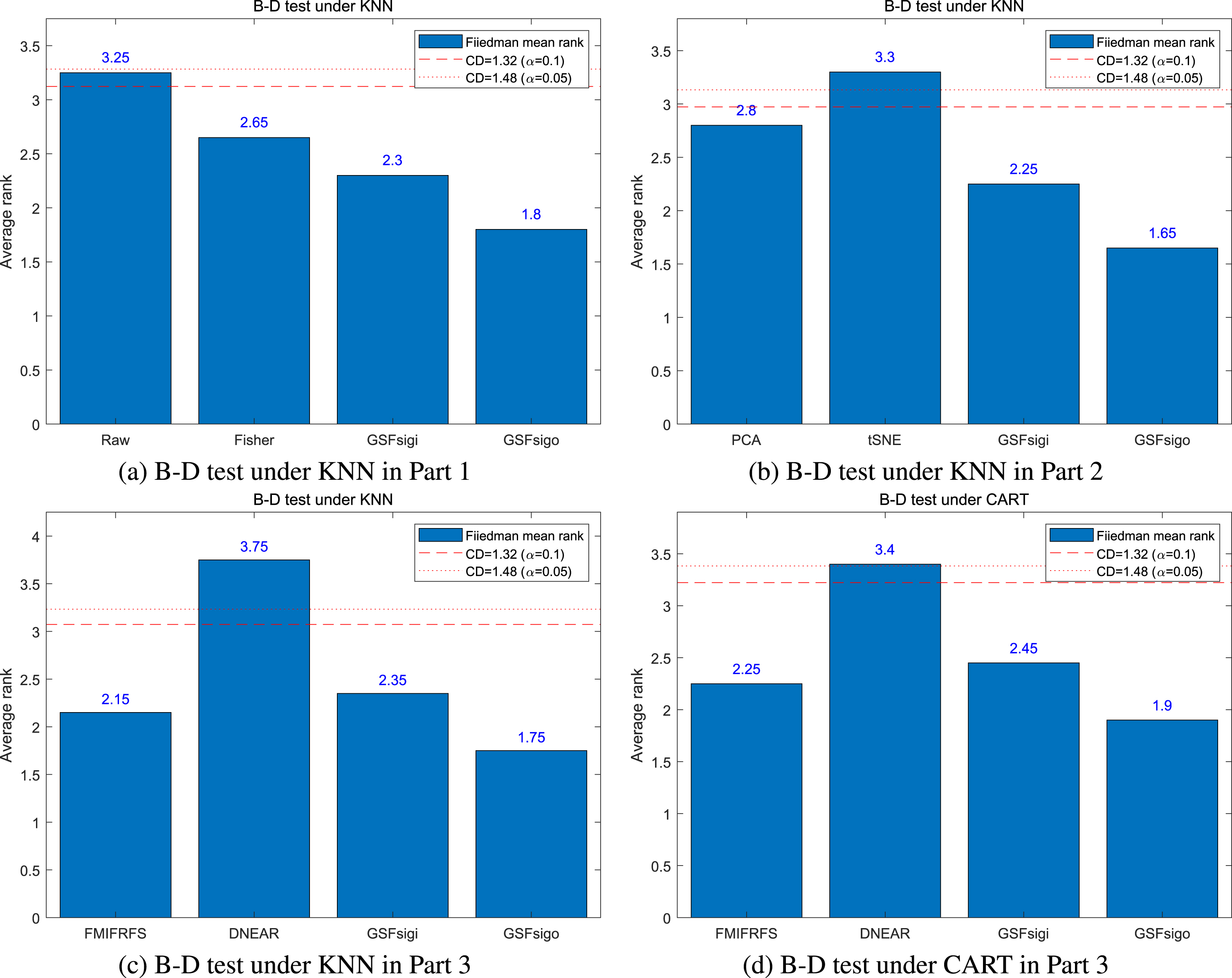
Bonferroni-Dunn test.

The lower histogram in Fig. 7 indicates a better rank. Analysis of Fig. 7(a) indicates that GSFsigo outperforms the raw data significantly at a significance level of α = 0.1 = 0.1. Additionally, there are no statistical differences among Fisher, GSFsigi, and GSFsigo under KNN classifier. Figure 7(b) demonstrates that GSFsigo performs significantly better than tSNE at α = 0.1 and 0.05, while PCA, GSFsigi and GSFsigo show no statistical differences under the KNN. In Fig. 7(c), GSFsigo is statistically significantly superior to DNEAR at at α = 0.1 and 0.05. Moreover, there are no statistical differences among FMIFRFS, GSFsigi, and GSFsigo unde KNN. Finally, Fig. 7(d) depicts that GSFsigo statistically significantly outperforms DNEAR at α = 0.1 and 0.05, while FMIFRFS, GSFsigi, and GSFsigo show no statistical differences under CART classifier.

6 Comparisons and discussions

To gain a better insight into the innovation of this paper, the section compares the proposed GSFsigi and GSFsigo with that of other related references.

1) Sharma et al. [35] proposed a C-HMOSHSSA framework for gene selection, combining the features of both Salp Swarm Algorithm (SSA) and Multi-Objective Spotted Hyena Optimizer (MOSHO). This hybrid algorithm was tested on seven high-dimensional datasets with four classifiers, using a subset of features (genes) obtained from the algorithm. The results showed that the proposed technique significantly outperformed the existing methods and identified new sets of informative and biologically relevant genes. The proposed approach can be applied to other problem domains that involve feature selection.

2) Bommert et al. [7] conducted a benchmark of filter methods for feature selection in high-dimensional gene expression survival data. They compared 14 filter methods across 11 data sets, aiming to provide guidance on the selection of filter methods for other researchers and practitioners. They assessed the accuracy of predictive models that used the selected features, as well as the run time, the number of features, and the selection stability. They discovered that the variance filter, which selects features with the highest variance without taking the survival outcome into account, outperformed the other methods. Additionally, the correlation-adjusted regression scores filter was identified as a more sophisticated alternative that allowed for models with similar predictive accuracy. Lastly, they studied filter methods based on feature rankings, finding groups of similar filters.

3) Sheng et al. [33] conducted a comprehensive study on the selection of gene features for unsupervised analysis of single-cell gene expression data. They provided a summary of 17 computational methods for gene feature selection, along with unified notations and statistical frameworks. This summary is beneficial for practitioners to choose the right method based on their assumptions and applicability, and for method developers to design new computational tools for unsupervised learning of scRNA-seq data. Additionally, they summarized the statistical frameworks used in single-cell gene selection for method developers.

4) Li et al. [22] conducted a study on gene selection in a single cell gene decision space using Gaussian kernel. They calculated the distance between two cells in each subspace of the single cell gene decision space, and then obtained the fuzzy T_cos-equivalence relation on the cell set based on the Gaussian kernel. Additionally, they examined measures of uncertainty for a single cell gene decision space and proposed information entropy and information granularity-based gene selection algorithms. To validate the algorithms, they tested them on several publicly available single cell RNA-seq data sets. The results showed that the algorithms could effectively select genes related to classification and significantly improve classification performances.

5) Sun et al. [38] proposed a novel method for tumor classification that utilizes neighborhood rough sets and entropy measure-based gene selection with Fisher score. This approach is capable of dealing with real-value data while preserving the original gene classification information. To reduce computation complexity, the Fisher score method was used to eliminate irrelevant genes. Additionally, some neighborhood entropy-based uncertainty measures were explored to address the uncertainty and noise of gene expression data. The properties of these measures were derived and the connections among them were established. Finally, a joint neighborhood entropy-based gene selection algorithm with the Fisher score was proposed to improve the classification performance of gene expression data. The results of experiments conducted on an instance and several public gene expression data sets showed that the proposed method is highly effective for selecting the most relevant genes with high classification accuracy.

6) In this paper, we examine gene selection in a gene decision space based on the concept of information entropy and consider its implications for gene expression data classification. To do this, we first establish the distance between two cells in the given decision subspace, and then define the binary relations induced by this decision subspace. We then investigate various information entropies for a gene decision space. Finally, we introduce several gene selection algorithms in a gene decision space by utilizing the information entropies presented. These algorithms are applied to gene expression data classifications and the results indicate that they are able to effectively select pertinent genes related to classifications and improve the classification performance considerably.

A comparison of this paper and the above related references are shown in Tables 14.

Table 13
The comparison of this paper with the above related references

Differences References Object Method Type of method Classifier Evaluation

Sharma et al. [35] microarray data SSA,MOSHO wrapper SVM, KNN, NBY, DT minimum Nfeature, maximum ACC

Bommert et al. [7] gene expression data - filter - maximum ARI

Sheng et al. [33] scRNA-seq data - filter,wrapper - -

Li et al. [22] scRNA-seq data FSigin, FSigout filter SVM, KNN, ELM minimum Nfeature, maximum ACC

Sun et al. [38] scRNA-seq data GSFSJNE filter SVM, KNN, C4.5 minimum Nfeature, maximum ACC

Our paper microarray data GSFsigi, GSFsigo filter KNN, CART minimum Nfeature, maximum ACC

Similarities (1) All these articles have investigated feature selection for gene expression data.

(2) All these articles have conducted machine learning methods to analyse the performance of feature selection.

(3) All these articles have the evaluation metric of minimum the number of features.

Differences	References	Object	Method	Type of method	Classifier	Evaluation
	Sharma et al. [35]	microarray data	SSA,MOSHO	wrapper	SVM, KNN, NBY, DT	minimum Nfeature, maximum ACC
	Bommert et al. [7]	gene expression data	-	filter	-	maximum ARI
	Sheng et al. [33]	scRNA-seq data	-	filter,wrapper	-	-
	Li et al. [22]	scRNA-seq data	FSigin, FSigout	filter	SVM, KNN, ELM	minimum Nfeature, maximum ACC
	Sun et al. [38]	scRNA-seq data	GSFSJNE	filter	SVM, KNN, C4.5	minimum Nfeature, maximum ACC
	Our paper	microarray data	GSFsigi, GSFsigo	filter	KNN, CART	minimum Nfeature, maximum ACC
Similarities	(1) All these articles have investigated feature selection for gene expression data.
	(2) All these articles have conducted machine learning methods to analyse the performance of feature selection.
	(3) All these articles have the evaluation metric of minimum the number of features.

Table 14

Semantic and abbreviations interpretation of Table 13

SSA	Salp Swarm Algorithm
MOSHO	multi-objective spotted hyena optimizer
SVM	Support Vector Machines
KNN	k-nearest neighbor
NBY	Naive Bayes
DT	Decision Tree
ELM	Extreme Learning Machine
CART	Classification And Regression Tree
Nfeature	number of features
ACC	classification accuracy
OL	ordered list
scRNA-seq	Single-cell RNA sequencing
ARI	adjusted Rand index
FSigin	Fisher score and inner-significance
FSigout	Fisher score and outer-significance
GSFSJNE	gene selection with Fisher score based on joint neighborhood
GSFsigi	Gene selections using Fisher score and inner-significances
GSFsigo	Gene selections using Fisher score and outer-significances

7 Conclusions

In this study, we have defined a gene decision space and the tolerance relations, and proposed some general information entropy. By utilizing λ-conditional information entropy, we have introduced the concepts of inner-significance and outer-significance for a gene decision space. We have presented two gene selection algorithms for a gene decision space. We have also presented two gene selection algorithms for this space. To evaluate the efficacy of these algorithms, we have applied them to gene expression data classifications using KNN and CART classifiers. Three measures, including gene number, RedR and ACC, are utilized to evaluate performances of algorithms. The obtained results performing on several publicly available gene expression datasets have demonstrated that the presented algorithms can select appropriate genes related to classification, and obviously or comparatively outperforms other competing approaches.

The advantages of this study are summarize as follows: (1) it has established a binary relation on the cell set of a decision subspace; (2) it has explored some information entropy in a gene decision subspace; (3) it has presented several gene selection algorithms in a gene decision space; and (4) it has validated the presentd algorithms using multiple public gene expression data sets.

These findings will be beneficial for boosting to gene engineering, target detection and biomedical engineering. We plan to ulteriorly promote these findings for practical engineering applications.

Acknowledgments

The authors would like to thank the editors and the anonymous reviewers for their valuable comments and suggestions, which have helped immensely in improving the quality of the paper. This work is supported by Natural Science Foundation of Guangxi Province (2021GXNSFAA220076, 2020GXNSFAA159155), Key Fields Project of Universities in Guangdong Province (2021ZDZX4109), and Scientific research platform of Guangdong Songshan Polytechnic (2022xjkypt02).

References

Azeem

, Imran

and Nadeem

M.F.

, Sharp bounds on partition dimension of hexagonal Möbius ladder, Journal of King Saud University –Science 34(2) (2022), 101779.

Azeem

, Jamil

M.K.

, Javed

and Ahmad

, Verification of SomeTopological Indices of Y-Junction Based Nanostructures byM-Polynomials, Journal of Mathematics 2022 (2022), 1–18.

Azeem

and Nadeem

M.F.

, Metric-based resolvability of polycyclic aromatic hydrocarbons, The European Physical Journal Plus, https://doi.org/10.1140/epjp/s13360-021-01399-8

Abdi

and Williams

L.J.

, Principal component analysis, Wiley Interdisciplinary Reviews: Computational Statistics 2 (2010), 433–459.

Beaubouef

, Petry

F.E.

and Arora

, Information-theoretic measures of uncertainty for rough sets and rough relational databases, Information Sciences 109 (1998), 185–195.

Blaszczynski

, Slowinski

and Szelag

, Sequential covering rule induction algorithm for variable consistency rough set approaches, Information Sciences 181(5) (2011), 987–1002.

Bommert

, Welchowski

, Schmid

and Rahnenfuhrer

, Benchmark of filter methods for feature selection inhigh-dimensional gene expression survival data, Briefings in Bioinformatics 23 (2022), bbab354.

Cament

L.A.

, Castillo

L.E.

, Perez

J.P.

, Galdames

F.J.

and Perez

C.A.

, Fusion of local normalization and Gabor entropy weighted features for face identification, Pattern Recognition 47(2) (2014), 568–577.

Cornelis

, Jensen

, Martin

G.H.

and Slezak

, Attribute selection with fuzzy decision reducts, Information Sciences 180 (2010), 209–224.

10.

Dunn

, Multiple comparisons among means, Journal of the American Statistical Association 56 (1961), 52–64.

11.

Dai

J.H.

, Hu

, Zheng

G.J.

, Hu

Q.H.

, Han

H.F.

and Shi

, Attribute reduction in interval-valued information systems based on information entropies, Frontiers of Information Technology and Electronic Engineering 17(9) (2016), 919–928.

12.

Dong

, Li

, Ding

and Sun

, A novel hybrid genetic algorithm with granular information for feature selection and optimization, Applied Soft Computing 65 (2018), 33–46.

13.

Dai

J.H.

, Xu

, Wang

W.T.

and Tian

H.W.

, Conditional entropy for incomplete decision systems and its application in data mining, International Journal of General Systems 41(7) (2012), 713–728.

14.

Friedman

, A comparison of alternative tests of significance for the problem of m rankings, The Annals of Mathematical Statistics 11 (1940), 86–92.

15.

Greco

, Inuiguchi

and Slowinski

, Fuzzy rough sets and multiple premise gradual decision rules, International Journal of Approximate Reasoning 41 (2006), 179–211.

16.

Jain

, Tiwari

A.K.

and Som

, A fitting model based intuitionistic fuzzy rough feature selection, Engineering Applications of Artificial Intelligence 89 (2020), 103421.

17.

Friedman

, A comparison of alternative tests of significance forthe problem of m rankings, The Annals of Mathematical Statistics 11 (1940), 86–92.

18.

, Sheng

V.S.

, Wang

Z.J.

, Ho

and Osman

, Incremental learning for v-support vector regression, Neural Networks 67 (2015), 140–150.

19.

Q.H.

, Pedrycz

, Yu

D.R.

and Lang

, Selecting discrete and continuous features based on neighborhood decision error minimization, IEEE Transactions on Systems, Man and Cybernetics (Part B) 40 (2010), 137–150.

20.

, Tsang

E.C.C.

, Guo

Y.T.

and Xu

W.H.

, Fast and robust attribute reduction based on the separability in fuzzy decision systems, IEEE Transactions on Cybernetics, doi: 10.1109/TCYB.2020.3040803.

21.

Jia

X.Y.

, Rao

, Shang

and Li

T.J.

, Similarity-based attributereduction in rough set theory: a clustering perspective, International Journal of Machine Learning and Cybernetics 11(2020), 1047–1060.

22.

Z.W.

, Feng

J.H.

, Zhang

, Liu

, Wang

and Wen

C.F.

, Gaussian kernel based gene selection in a single cell gene decision space, Information Sciences 610 (2022), 1029–1057.

23.

Z.W.

, Liu

X.F.

, Zhang

G.Q.

, Xie

N.X.

and Wang

S.C.

, Amulti-granulation decision theoretic rough set method fordistributed fc-decision information systems: An applicationinmedical diagnosis, Applied Soft Computing 56 (2017), 233–244.

24.

Z.W.

, Qu

L.D.

, Zhang

G.Q.

and Xie

N.X.

, Attribute selection for heterogeneous data based on information entropy, International Journal of General Systems 50(5) (2021), 548–566.

25.

, Zhang

and Ogihara

, A comparative study of feature selection and multiclass classification methods for tissue classification based on gene expression, Bioinformatics 20 (2004), 2429–2437.

26.

Z.W.

, Zhang

P.F.

, Ge

, Xie

N.X.

, Zhang

G.Q.

and Wen

C.F.

, Uncertainty measurement for a fuzzy relation information system, IEEE Transactions on Fuzzy Systems 27 (2019), 2338–2352.

27.

Maji

, Rough hypercuboid approach for feature selection in approximation spaces, IEEE Transactions on Knowledge and Data Engineering 99 (2012), 1–14.

28.

Navarrete

, Viejo

and Cazorla

, Color smoothing for RGB-Ddata using entropy information, Applied Soft Computing 46 (2016), 361–380.

29.

Pawlak

, Rough sets: Theoretical aspects of reasoning about data, Kluwer Academic Publishers, Dordrecht, 1991.

30.

Rao

, Shi

, Rodrigue

A.K.

, Feng

, Xia

, Elhoseny

, Yuanand

and Gu

, Feature selection based on artificial bee colony andgradient boosting decision tree, Applied Soft Computing 74 (2019), 634–642.

31.

Shannon

, A mathematical theory of communication, Bell SystemTechnical Journal 27 (1948), 379–423.

32.

Seijo-Pardo

, Bolón-Canedo

and Alonso-Betanzos

, Ondeveloping an automatic threshold applied to feature selectionensembles, Information Fusion 45 (2019), 227–245.

33.

Sheng

and Li

W.V.

, Selecting gene features for unsupervisedanalysis of single-cell gene expression data,bbab, Briefings inBioinformatics 22 (2021), 295.

34.

de Souza

R.C.T.

, de Macedo

C.A.

, Dos Santos Coelho

, Pierezan

and Mariani

V.C.

, Binary coyote optimization algorithm for feature selection, Pattern Recognition 107 (2020), 107470.

35.

Sharma

and Rani

, C-HMOSHSSA: Gene selection for cancer classification using multi-objective meta-heuristic and machine learning methods, Computer Methods and Programs in Biomedicine 178 (2019), 219–235.

36.

Singh

, Shreevastava

, Som

and Somani

, A fuzzy similarity-based rough set approach for attribute selection inset-valued information systems, Soft Computing 24(2020), 4675–4691.

37.

Shukla

A.K.

, Singh

and Vardhan

, A hybrid gene selection method for microarray recognition, Biocybernetics and Biomedical Engineering 38 (2018), 975–991.

38.

Sun

, Zhang

X.Y.

, Qian

Y.H.

, Xu

J.C.

, Zhang

S.G.

and Tian

, Joint neighborhood entropy-based gene selection method with fisher scorefor tumor classification, Applied Intelligence 49(2019), 1245–1259.

39.

Sun

, Zhang

, Qian

, Xu

and Zhang

, Feature selection using neighborhood entropy-based uncertainty measures for gene expression data classification, Information Sciences 502(2019), 18–41.

40.

Tan

A.H.

, Shi

S.W.

, Wu

W.Z.

, Li

J.J.

and Pedrycz

, Granularity and entropy of intuitionistic fuzzy information and their applications, IEEE Transactions on Cybernetics, doi: 10.1109/TCYB.2020.2973379.

41.

Thangavel

and Pethalakshmi

, Dimensionality reduction based onrough set theory: A review, Applied Soft Computing 9(2009), 1–12.

42.

Van der Maaten

and Hinton

, Visualizing data using t-SNE, Journal of Machine Learning Research 9 (2008), 2579–2605.

43.

Wierman

M.J.

, Measuring uncertainty in rough set theory, International Journal of General Systems 28 (1999), 283–297.

44.

Wang

Y.B.

, Chen

X.J.

and Dong

, Attribute reduction via local conditional entropy, International Journal of Machine Learningand Cybernetics 10(12) (2019), 3619–3634.

45.

Wnag

C.Z.

, Wang

, Shao

M.W.

, Qian

Y.H.

and Chen

D.G.

, Fuzzy rough attribute reduction for categorical data, IEEE Transactions on Fuzzy Systems 28 (2020), 818–830.

46.

Wang

, Zhang

P.F.

and Li

Z.W.

, A three-way decision method based on Gaussian kernel in a hybrid information system with images: An application in medical diagnosis, Applied Soft Computing 77 (2019), 734–749.

47.

, Song

, Min

, Lai

and Zheng

, Joint adaptive manifold and embedding learning for unsupervised feature selection, Pattern Recognition 112 (2021), 107742.

48.

Wang

, Zhang

, Sun

, Wang

and Du

, Multi-objective feature selection based on artificial bee colony: An acceleration approach with variable sample size, Applied Soft Computing 88 (2020), 106041.

49.

Xie

S.D.

and Wang

Y.X.

, Construction of tree network with limited delivery latency in homogeneous wireless sensor networks, Wireless Personal Communications 78(1) (2014), 231–246.

50.

Yang

X.B.

, Yu

D.J.

, Yang

J.Y.

and Wei

, Dominance-based rough set approach to incomplete interval-valued information system, Dataand Knowledge Engineering 68(11) (2009), 1331–1347.

51.

Yang

, Liu

Y.L.

, Feng

C.S.

and Zhu

G.Q.

, Applying Fisher score toidentify Alzheimer’s disease-related genes, Genetics and Molecular Research 15 (2016), 1–9.

52.

Zhang

G.Q.

, Li

Z.W.

, Wu

W.Z.

, Liu

X.F.

and Xie

N.X.

, Information structures and uncertainty measures in a fully fuzzy information system, International Journal of Approximate Reasoning 101 (2018), 119–149.

53.

Zeng

A.P.

, Li

T.R.

, Liu

, Zhang

J.B.

and Chen

H.M.

, A fuzzy roughset approach for incremental feature selection on hybrid information systems, Fuzzy Sets and Systems 258 (2015), 39–60.

54.

Zhang

, Zhang

G.Q.

, Li

Z.W.

, Qu

L.D.

and Wen

C.F.

, Features election in a neighborhood decision information system with application to single cell RNA data classification, Applied Soft Computing 113 (2021), 107876.