Application of an improved VGG and RPN network in precision parts recognition

Abstract

Although various automatic or semi-automatic recognition algorithms have been proposed for tiny part recognition, most of them are limited to expert knowledge base-based target recognition techniques, which have high false detection rates, low recognition accuracy and low efficiency, which largely limit the quality as well as efficiency of tiny part assembly. Therefore, this paper proposes a precision part image preprocessing method based on histogram equalization algorithm and an improved convolutional neural network (i.e. Region Proposal Network(RPN), Visual Geometry Group(VGG)) model for precision recognition of tiny parts. Firstly, the image is restricted to adaptive histogram equalization for the problem of poor contrast between part features and the image background. Second, a custom central loss function is added to the recommended frame extraction RPN network to reduce problems such as excessive intra-class spacing during classification. Finally, the local response normalization function is added after the nonlinear activation function and pooling layer in the VGG network, and the original activation function is replaced by the Relu function to overcome the problems such as high nonlinearity and serious overfitting of the original model. Experiments show that the improved VGG model achieves 95.8% accuracy in precision part recognition and has a faster recognition speed than most existing convolutional networks trained on the same test set.

Keywords

Precision parts histogram equalization image recognition VGG RPN

1 Introduction

In recent decades, there has been an increasing demand for manufacturing products and higher requirements for product quality, and at the same time, precision micro and small electromechanical products obtained through micro-assembly have a compact structure, a small size, stable performance, low energy consumption, and strong anti-interference capability [1]. At present, although the micro parts assembly technology based on machine vision has been applied to various fields and industries, the technology is not mature, and the more important microelectromechanical sensor parts are still assembled manually on the production lines of various industries in China [2]. Therefore, the research of micropart identification technology is of great significance for the liberation of manpower and the realization of high-efficiency and high-quality automated assembly of microparts.

In micro assemblies where tiny parts are mostly rigid, image-matching recognition algorithms are generally used [3 –6], which can be divided into matching algorithms based on grayscale information and feature-based matching algorithms. Grayscale information-based matching algorithms [7, 8] recognize the target by comparing the similarity of the grayscale values of the pixel points of the template image and the target image, and these algorithms are better for the recognition of images with complex patterns and images with small changes in grayscale values, with the disadvantage that the computation is relatively large and very sensitive to nonlinear changes in illumination; feature-based matching algorithms first extract the target image and the template image special shapes [9, 10], such as corner points, spots, contours and other shapes, and then a recognition algorithm that matches by comparing the similarity of features. In this regard, Ma et al. proposed the SC-GHT (Sobel Candy Generalized Hough Transform, SC-GHT) matching algorithm [11], which uses the curvature of the target contour edge as well as the gradient for matching; Ser et al. proposed the RG-GHT (Rotation Gradients Generalized Hough Tranform (RG-GHT) algorithm [12], which first uses edge point pairs to build a lookup table and then matches by looking up the table, this algorithm does not match well when the target edge points are occluded, so Thomas et al. improved the indexing of the lookup table [13] by using the offset vector as the index of the lookup table; Kassim et al. proposed the DV-GHT (Displacement Vecter Generalized Hough Transform, DV-GHT) algorithm [14], which solves the problem of matching failure due to target rotation as well as dimensional changes, but is susceptible to noise as well as illumination changes. Feature point matching-based algorithm is an algorithm that matches by finding the correlation between the target image and the template image descriptors [15], such as the SIFT (Scale-invariant Feature Transform, SIFT) algorithm proposed by Lowe et al. [16], which uses a Gaussian scale space constructed by a pyramid strategy for feature point matching with better rotation invariance and scale invariance; to solve the problem of high time complexity of the SIFT algorithm, Herbert et al. proposed the SURF (Speeded Up Robust Features, SURF) algorithm [17], which uses box filtering to approximate the Gaussian function. Both of the above-mentioned algorithms have certain defects in constructing the size space, as Gaussian filtering removes the boundary information of the target and smoothes the details and noise to the same extent at the same scale, which seriously affects the accuracy of recognition; to address the defects of Gaussian kernel function in constructing the size space, Alcantarilla et al. proposed a wind (KAZE) algorithm using nonlinear diffusion filtering [18], which solves nonlinear diffusion equations by AOS (Additive Operator Splitting, AOS) numerical approximation [19], which is stable and parallelizable, but the drawback is that it requires solving large linear systems of equations and the recognition speed is relatively slow.

As the performance of image processors (Graphics Processing Unit, GPU) [20, 21] improves, convolutional neural networks are becoming increasingly superior for target detection tasks. The target recognition algorithms based on convolutional neural networks are mainly divided into two categories, one is the one-stage algorithm, which directly classifies and regresses images, and the YOLO (You Look Only Once, YOLO) algorithm proposed by Joseph Redmon et al. [22] is one of the representative works. Another class is the two-stage algorithm, which first needs to select the recommendation frame of the image, and then classify and regress the recommendation frame. The Faster R-CNN (Faster Region Convolutional Naural Network, Faster R-CNN) algorithm proposed by Kai-Ming He et al. [23] and the Mask R-CNN (Mask Region Convolutional Naural Network, Mask R-CNN) proposed by Kai-Ming He et al. The Network (Mask R-CNN) algorithm [24] belong to the two-stage class, among which the RPN (Region Proposal Network, RPN) network used for recommendation frame extraction in the Faster R-CNN algorithm is still widely used nowadays. The one-stage class algorithm only needs one step to achieve the target. The one-stage algorithm is faster than the two-stage algorithm, but it is not accurate enough.

DL algorithms represented by convolutional neural networks (CNN) can learn features directly from a large number of raw data sets without a tedious pre-processing process, and the speed and accessibility of computation are greatly improved. Compared with traditional ML algorithms, CNN algorithms have been widely used in image recognition in recent years due to their remarkable performance [25 –27]. VGG networks, as one of the CNN algorithms, have demonstrated that deeper network layers can effectively extract richer classification images with higher accuracy [28 –31]. However, building a good CNN model requires a large dataset, especially for precision engineering, where the acquisition of tiny mechanical part images is more challenging due to size, environment, and similar parts.

To address the problem of small part samples, some researchers have trained models directly with a limited number of images and improved the robustness of classification by optimization algorithms [32, 33], while others have used data augmentation to extend the tiny part dataset [34 –36]. However, regardless of the method used to construct the dataset, data preprocessing is performed before constructing the tiny parts dataset, considering the interference of the external environment on the image dataset [37 –39]. The main image preprocessing is done by image contrast enhancement, noise removal, and data normalization to achieve the best quality of the dataset. Traditional methods of image contrast enhancement, such as histogram equalization, and adaptive histogram equalization still suffer from the problem of local contrast being over-amplified to the point of image distortion, and due to the use of local histogram equalization, there is the problem of blocky images. In contrast, the improved histogram equalization method proposed in this paper achieves the ideal effect to solve the problem of image distortion and background whitening caused by high local contrast. Meanwhile, this paper adopts the features extracted by a convolutional neural network for recognition, which has better rotational as well as scale invariance. Feature fusion can solve the problem of inaccurate or unrecognizable micro- and small-parts recognition, and the problem that recognition speed cannot be real-time is solved by improving the structure of the convolutional kernel in a convolutional neural network. The central loss function is added to the convolutional neural network model training to reduce the correlation between the part features and solve the interference problem of similar parts, etc.

2 Image acquisition system design

The main research object of this paper is mechanical table parts with sizes between 0.1 5 mm, and the purpose is to use image recognition technology for real-time non-contact recognition of tiny parts in micro-assembly. Building a tiny part recognition system as the basis, the workflow of the design recognition system is shown in Fig. 1.

Fig. 1

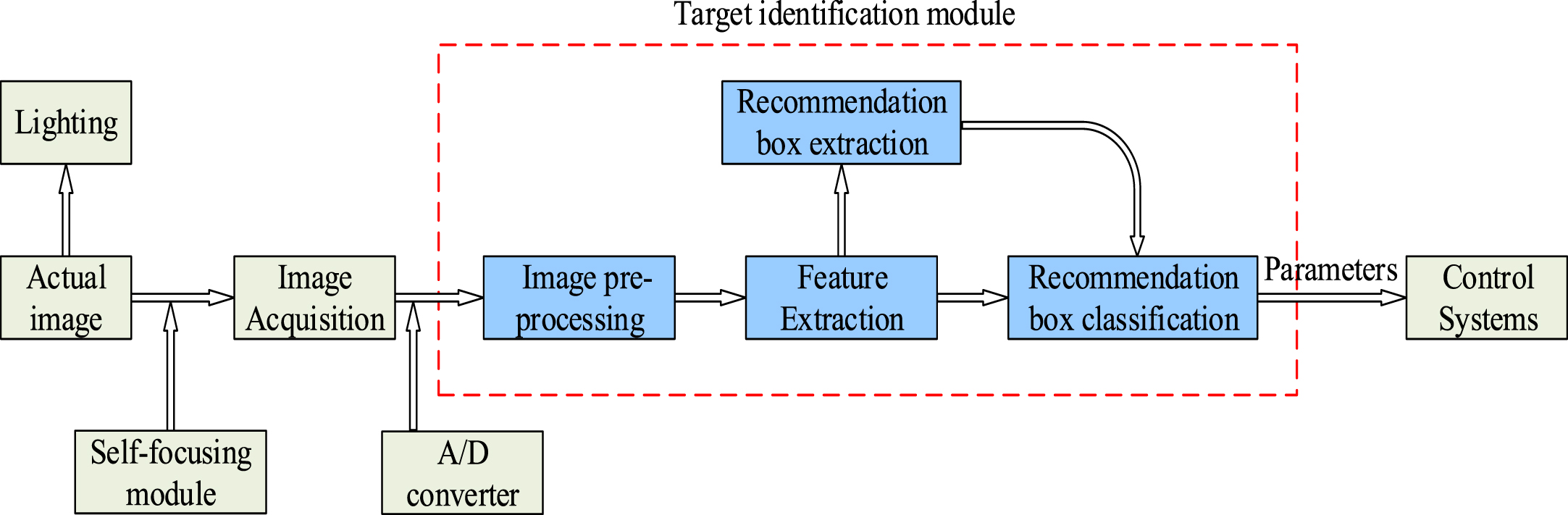
Workflow of the target recognition system.

2.1 Identification system composition

The microscopic part recognition system consists mainly of a microscopic vision image acquisition module, an auto-focus module, a microscopic vision image processing module, a computer control module, and an actuator module. The overall structure of the visual recognition system is shown in Fig. 2.

Fig. 2

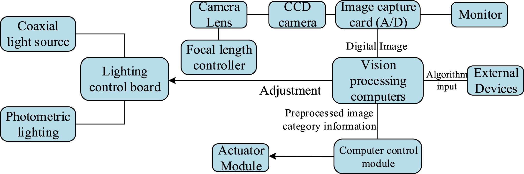
Structure diagram of the target recognition system.

2.2 Experimental platform construction and image acquisition

The experimental platform is mainly composed of a computer, mobile table, CCD camera, lens, and light source, and the tiny parts identification experimental platform is shown in Fig. 3.

Fig. 3

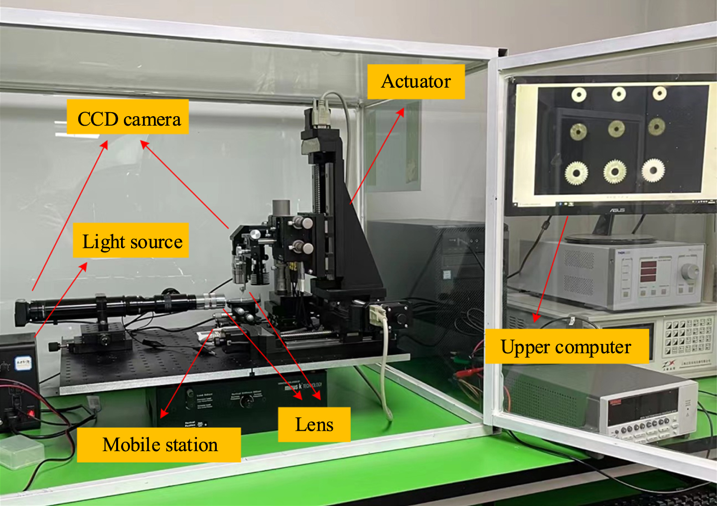
Experiment platform of micro parts recognition.

Among them, the CCD camera is the main part of the image acquisition module, which is a faceted unit composed of semiconductor components that have a photoelectric conversion function, and each semiconductor component stores the amount of charge that can sense the image signal and can output that charge in the order of the control signal, thus forming an electrical signal. Eventually, the optical signal is converted into a digital signal and transmitted to a computer for the next step of processing. The camera model used in this paper is the Boshioda U-300, CCD camera. Its main performance indicators and parameters are shown in Table 1.

Table 1

Main performance and parameters of the BOSHIDA U-300

Performance Indicators	Parameters
Camera Model	BOSHIDA U-300
Sensor Model	1/2 inch, CMOS gray
Framerate	30fps@ 1024 × 1024
Pixel depth	8bit
Pixel size	3.2μm×3.2μm
External size	50mm×50mm×40mm
Stable temperature	0–50°C

3 Image pre-processing and data set building

When the identification system is working, the industrial CCD camera and the microscope head get the original picture of the part to be assembled. According to the clarity of the picture, the distance between the actual picture and the microscope head is adjusted to make the best effect of imaging and to realize the automatic focus alignment of the optical system. In addition, before the recognition of the parts in the picture, the picture is denoised as well as enhanced with data processing to avoid some unnecessary external interference. The pre-processed images are annotated, and the image data set is expanded (i.e., rotated, contrast reduced, etc.) to solve the problem of difficult manual annotation.

3.1 Improved histogram equalization

Problems such as lack of contrast between the part and the background due to insufficient light, reflections, or the ability of the part itself to reflect light. Figure 4 shows the part image captured by the image recognition system.

Fig. 4

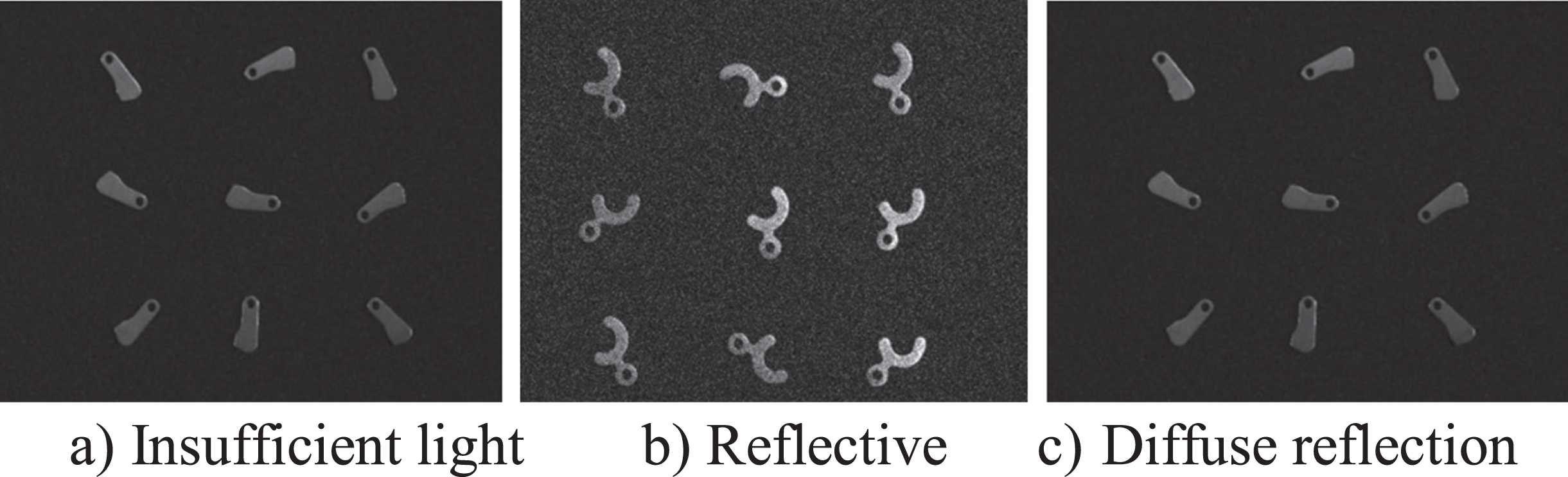
Original parts acquisition drawings.

From Fig. 5 b), it can be found that when the contrast between parts and background is not high, the histogram gray level of the image is concentrated between [0,25], which makes the whole image behave darker and is not conducive to the subsequent recognition of the parts, so the histogram equalization operation is performed to make the histogram cover as many gray levels as possible and distribute as evenly as possible.

Fig. 5

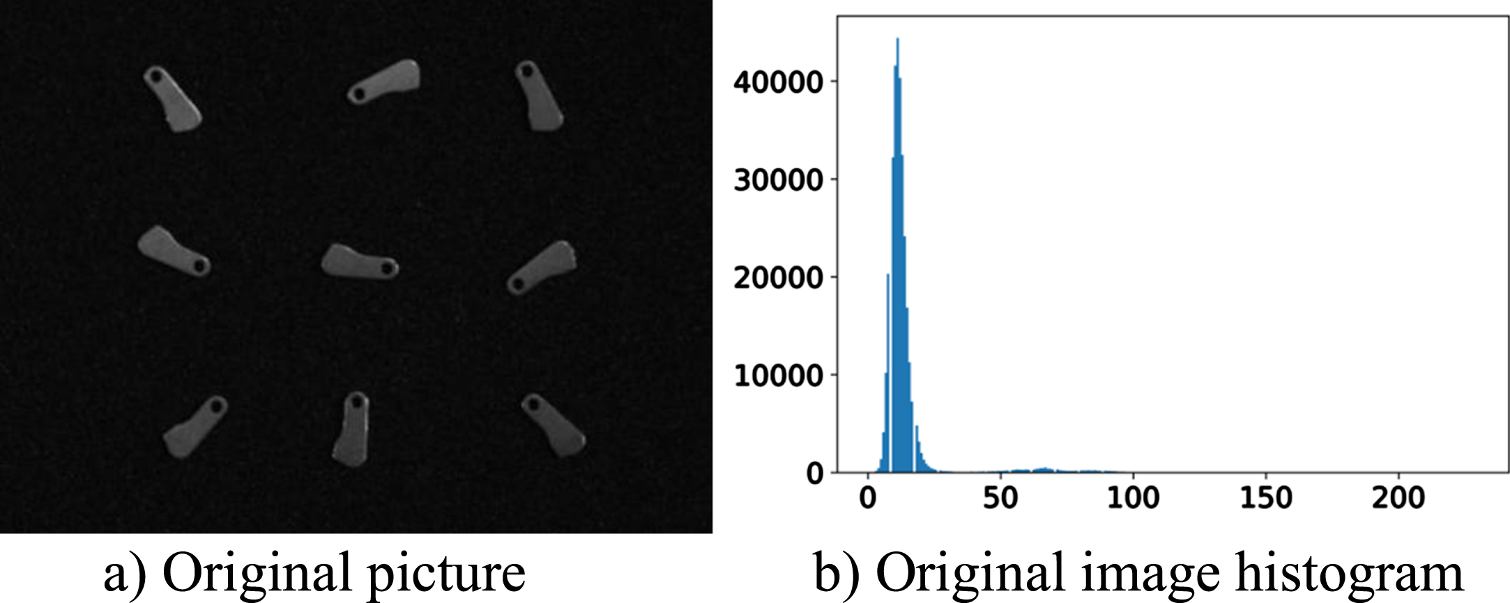
Original image and histogram.

Histogram equalization is a pixel-level image processing method [40 –42], which is implemented by the following nonlinear transformation function: $s - T (r), 0 < = r < = 1$ (1)

Where r is the pixel value before the transform, s is the pixel value after the transform, and T is the transform function, which is single-valued and monotonically increasing on the defined interval [0,255], the role of the single-valued is to ensure the existence of the image recovery function after the transform. The monotonically increasing function is to make the original image and the transformed image order-preserving, avoiding the black-and-white inversion of the image before and after the transformer. Let p_r (r) and p_s (s) be the probability density functions of the pixel values before and after the transformer, respectively, the probability that the gray levels are between [0,n] before and after the transformer is: $S, (n) = \int_{0}^{n} p_{r} (r) dr$ (2) $S_{s} (n) = \int_{0}^{n} p_{s} (s) ds$ (3)

To ensure the order-preserving gray levels before and after the transformation and to avoid the black-and-white inversion, it is necessary to make S_r (n) = S_s (n), therefore: $p_{r} (r) dr = p_{s} (s) ds$ (4)

The transformation function used in this paper is given by the following equation: $s = T (r) = \int_{0}^{r} p_{r} (w) dw$ (5)

Derivation on both sides of the equal sign yields: $\frac{ds}{dr} = \frac{dT (r)}{dr} = p_{r} (r)$ (6)

Combining Equations (6) yields: $p_{s} (s) = p_{r} (r) \frac{1}{p_{r} (r)} = 1$ (7)

Because the probability density function of the gray level s after transformation is a constant on the interval [0,255], s satisfies the uniform distribution, and the transformation function used in this paper is valid. After discretizing the transform function, we get: $\begin{matrix} S_{k} = T (r_{k}) = \sum_{j = 0}^{k} p_{r} (r_{j}) \\ = \sum_{j = 0}^{k} \frac{n_{j}}{n}, k = 0, 1, 2, \dots, 255 \end{matrix}$ (8)

Figure 6 a) shows the image after histogram equalization, and Fig. 6 b) shows the histogram of the image after histogram equalization. Although the gray levels are uniformly distributed and the contrast of the parts is significantly enhanced after the transformation, the image shows the phenomenon of excessive local contrast enhancement, which makes the image distorted. Figures 6 c) and d) show the images after adaptive histogram equalization and their histograms. The adaptive histogram equalization still has the problem that the local contrast is over-enhanced to the extent that the image is distorted, and the image is blocky due to the local histogram equalization. Because the background of the image is completely black, i.e., the histogram of the image has a high magnitude at the 0 gray level, which leads to a high slope of the mapping function here, the gray values obtained by the mapping function are mapped to the right side of the histogram, so the background of the image becomes white after the adaptive histogram equalization.

Fig. 6

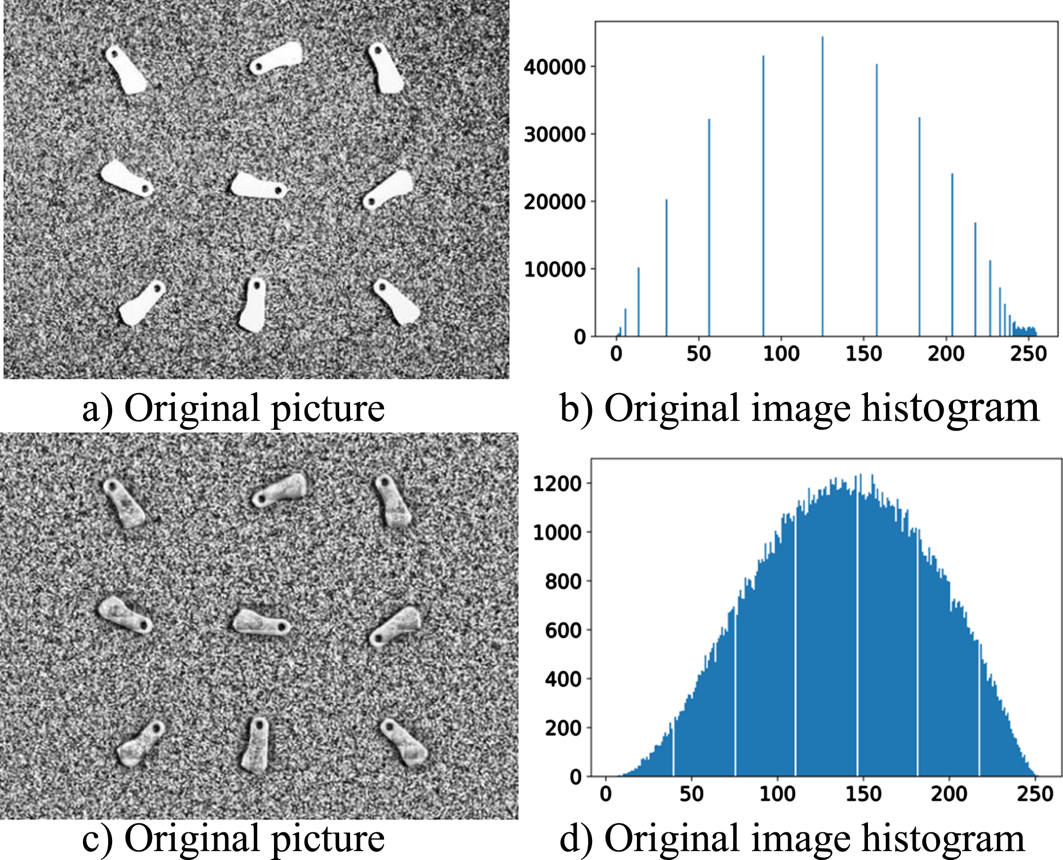
Histogram equalization and histogram.

To solve the problems of image distortion and background whitening caused by the high local contrast of the image, the histogram of each sub-block is cropped to indirectly limit the slope of the transform function so that the gray values obtained by the mapping function are mapped to the left side of the histogram. The improved histogram is shown in Fig. 7, where the part of the histogram above a certain threshold is cropped off, and the cropped part is evenly distributed below the histogram to ensure that the area of the whole histogram remains unchanged.

Fig. 7

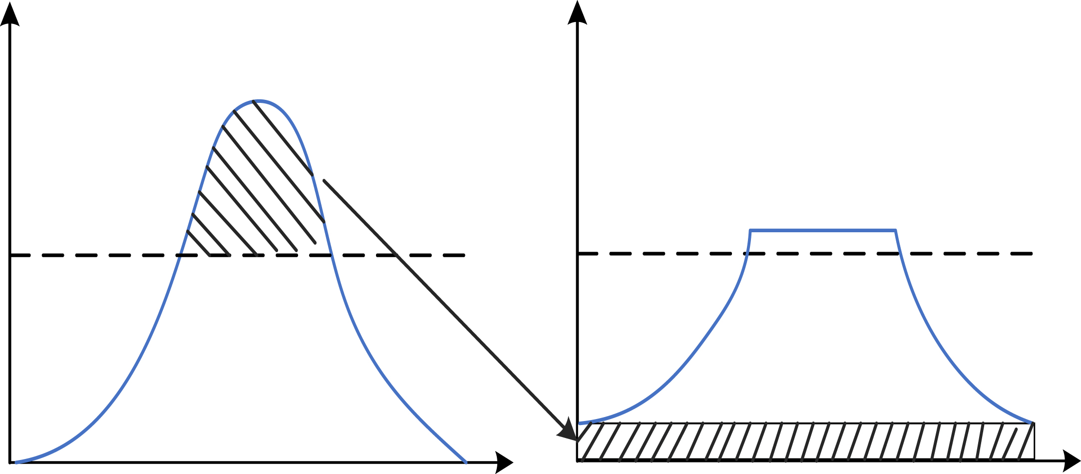
Histogram clipping.

To solve the problem of blocky images, this paper uses a bilinear interpolation method for images. First, the whole image is divided into small blocks, and each block is equalized by a histogram. The pixel values in the top corners are not changed, and the pixel values in the edge regions are obtained by bilinear interpolation of two adjacent edge blocks, and the pixel points in the middle regions are obtained by bilinear interpolation of the surrounding four blocks.

Figure 8 a) shows the image after the improved histogram equalization, and Fig. 8 b) shows the histogram of this image. It can be found that both of the above problems have been solved, and the contrast of the image has been significantly improved.

Fig. 8

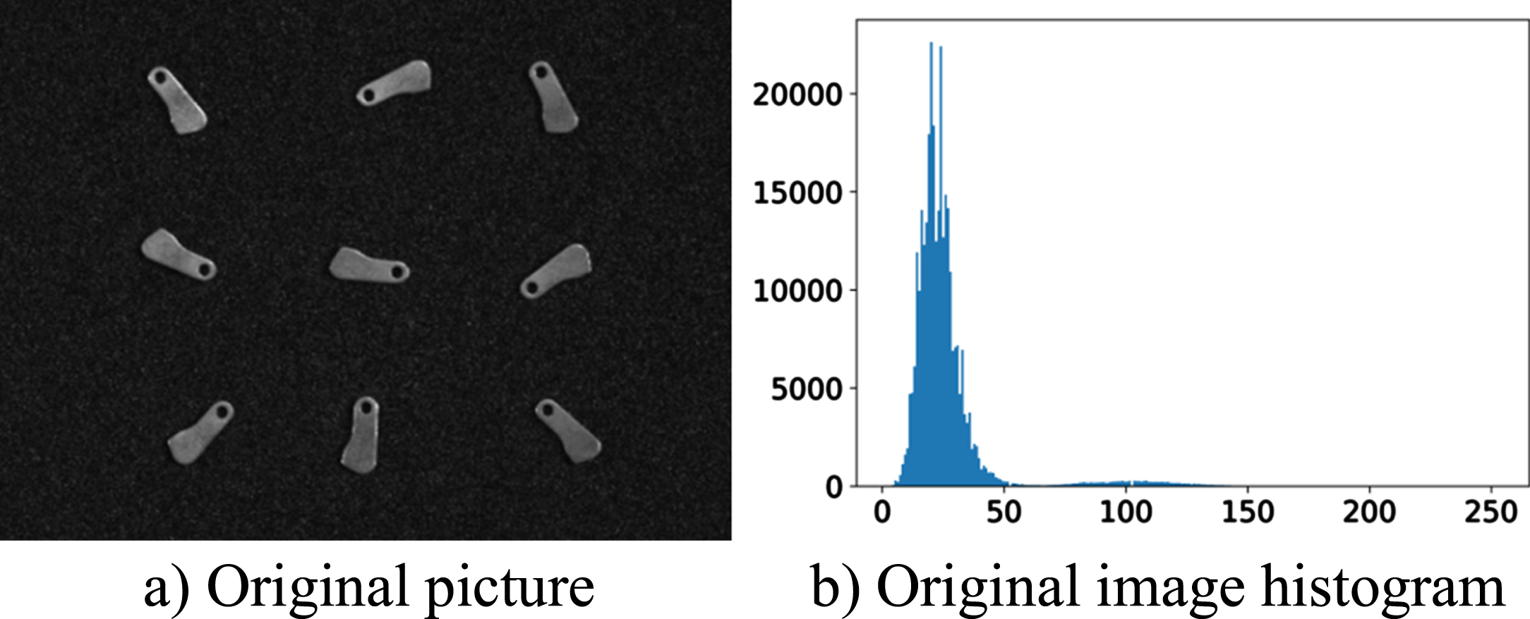
Limited adaptive histogram equalization and its histogram.

3.2 Image filtering and data normalization

Feature extraction of part images using convolutional neural networks relies on a large dataset, and the high temperature of the camera sensor during a long time of image acquisition can cause the acquired images to generate unwanted noise. The methods for noise removal in the spatial domain are generally classified as linear and nonlinear filtering [43 –46]. Among them, linear filtering using the weighted average method can ensure the directional symmetry of the filter as well as the uniqueness of the peak, Fig. 9 a) shows the mean filter and Fig. 9 b) shows the effect of the mean filter after the mean filter. From the images, it can be found that the mean filter is not effective for this type of noise. In this paper, the Gaussian filter in nonlinear filtering is used, and the Gaussian filter is deduced from Equation (9):

Fig. 9

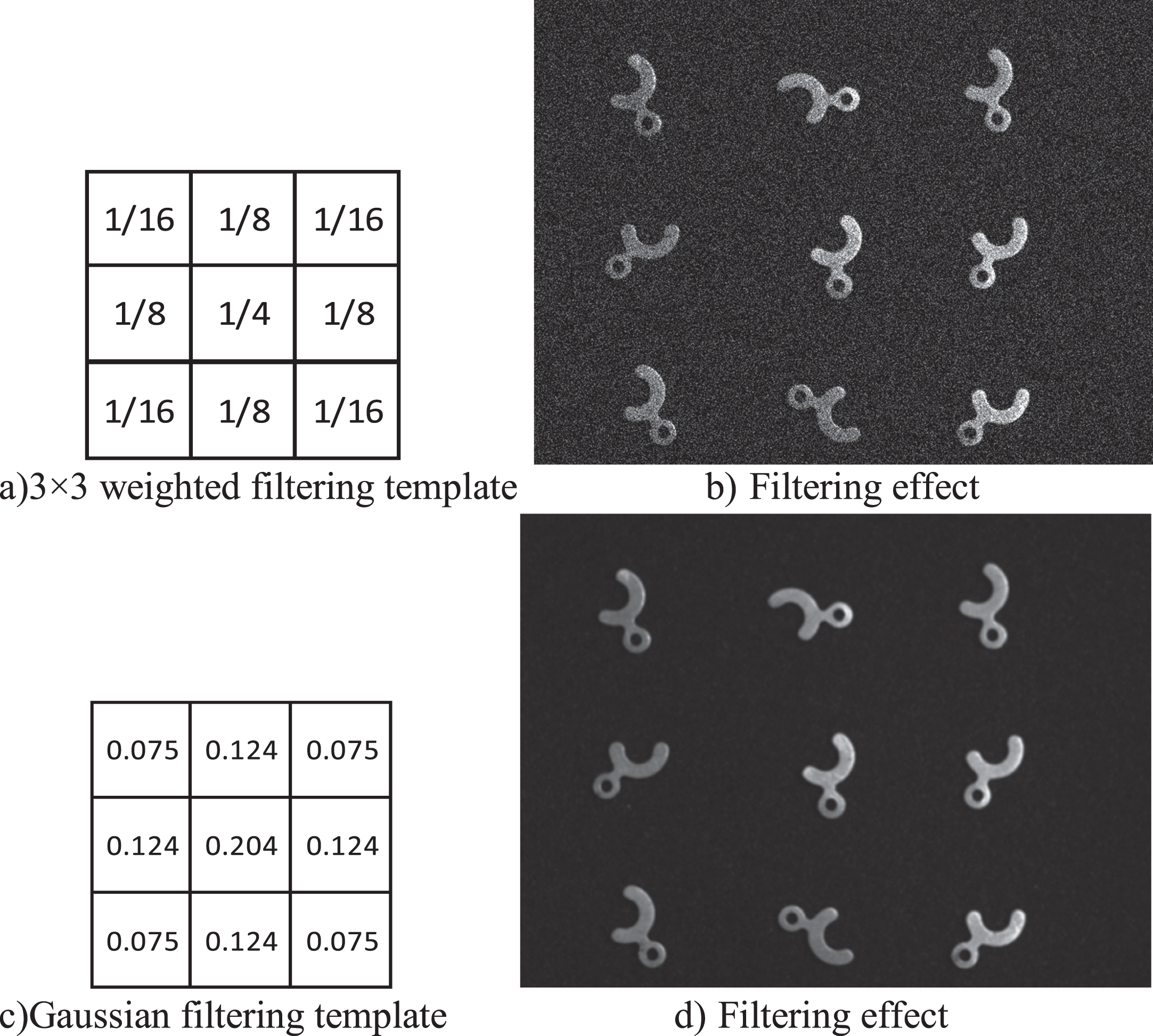
Comparison of filtering effect.

$f (x) = \frac{1}{(\sqrt{2 π} σ)^{2}} e^{- (x - u)^{2} / 2 σ^{2}}$ (9)

The Gaussian filter is two-dimensional, so the function can be transformed into a two-dimensional function by turning Equation (9) into a vector. Where is the position of any point in the filter, is the coordinates of the center point of the filter, Fig. 9 c) shows the Gaussian filter template, and Fig. 9 d) shows the effect after Gaussian filtering. As shown in Fig. 9 d), although the image becomes slightly blurred, the effect of noise removal is very good. From the experiment, we can find that the image noise generated by the camera sensor overheating is Gaussian noise, which can be removed by a Gaussian filter.

When there is a large gap in the data, the objective function is in a narrow ellipse when the parameter gradient is updated (as shown in Fig. 10 a)), where the direction of the gradient is in the direction of the vertical contour, and the parameter update is slower. After normalization, the objective function becomes more regular (as shown in Fig. 10 b)), and the parameter update becomes faster.

Fig. 10

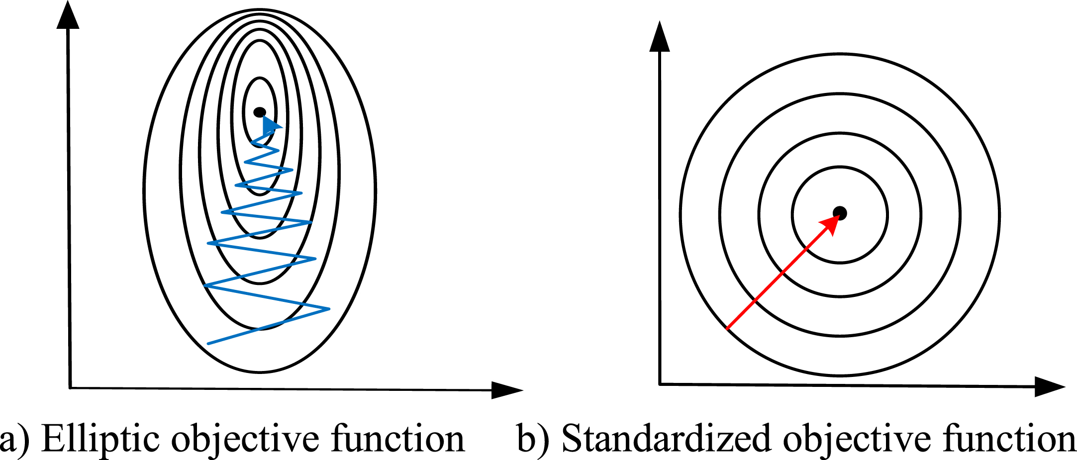
Parameter gradient descent diagram.

Generally, the deeper the network is, the better the detection effect is under reasonable parameter tuning. However, the deeper convolutional neural network has a great dependence on the dataset, and the time cost of manual labeling is high, so the dataset needs to be expanded. As shown in Fig. 11 a), b) and c) are the original, reduced contrast and rotated images respectively, the data set expansion is achieved through the following series of operations.

Fig. 11

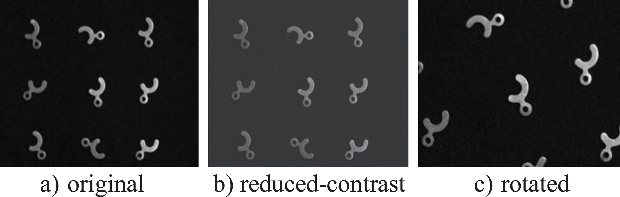
Process of data augmentation.

4 Convolutional neural network recognition algorithm network improvement

4.1 VGG network model improvement

The VGG network model has a substantially larger number of neurons in the accessed fully connected layers due to the increase in the input size, which makes the nonlinearity of the network more pronounced, with more categories to be classified and higher accuracy [47, 48]. However, there are still problems such as long training time and difficulty in tuning the parameters on precision-level target recognition tasks.

To avoid the problems caused by these limitations in a tiny target recognition, this paper removes the LRN layer in VGG and uses the Dropout layer to solve the overfitting problem. Although the LRN layer improves the generalization ability of the model to a certain extent, the recognition rate is only improved by 1 2% and the computation is more complicated. The principle of Dropout is to randomly delete some neurons of the layer, which reduces the nonlinearity of the model and avoids the overfitting of the model. In addition, the strategy for selecting convolutional kernels in the VGG network is to use multiple small convolutional kernels instead of one large convolutional kernel. There are two main reasons for this operation, one is that increasing the number of layers of the network can improve the nonlinear expression ability of the network, and then improve the accuracy of the model. Second, the number of parameters has been reduced, two 3 × 3 convolution kernels and a 5 × 5 convolution kernel parameter ratio of 3 × 3 × 2/(5 ×5) =0 . 72, three 3 × 3 convolution kernels and a 7 × 7 convolution kernel parameter ratio of 3 × 3 × 3/(7 ×7) =0.55, the number of parameters has been reduced by nearly double, the improvement effect is obvious. The improved VGG network model structure and the overall microsystem recognition flow chart are shown in Fig. 12, which intuitively demonstrates the improvement and recognition process. Table 2 shows the comparison of the accuracy and the number of parameters between this network and the other four classical network models. The number of parameters of this network is lower, but the accuracy is not much different from that of VGG16 and Inception-v3, so the depth-level separable convolution can significantly improve the recognition speed while ensuring accuracy.

Fig. 12

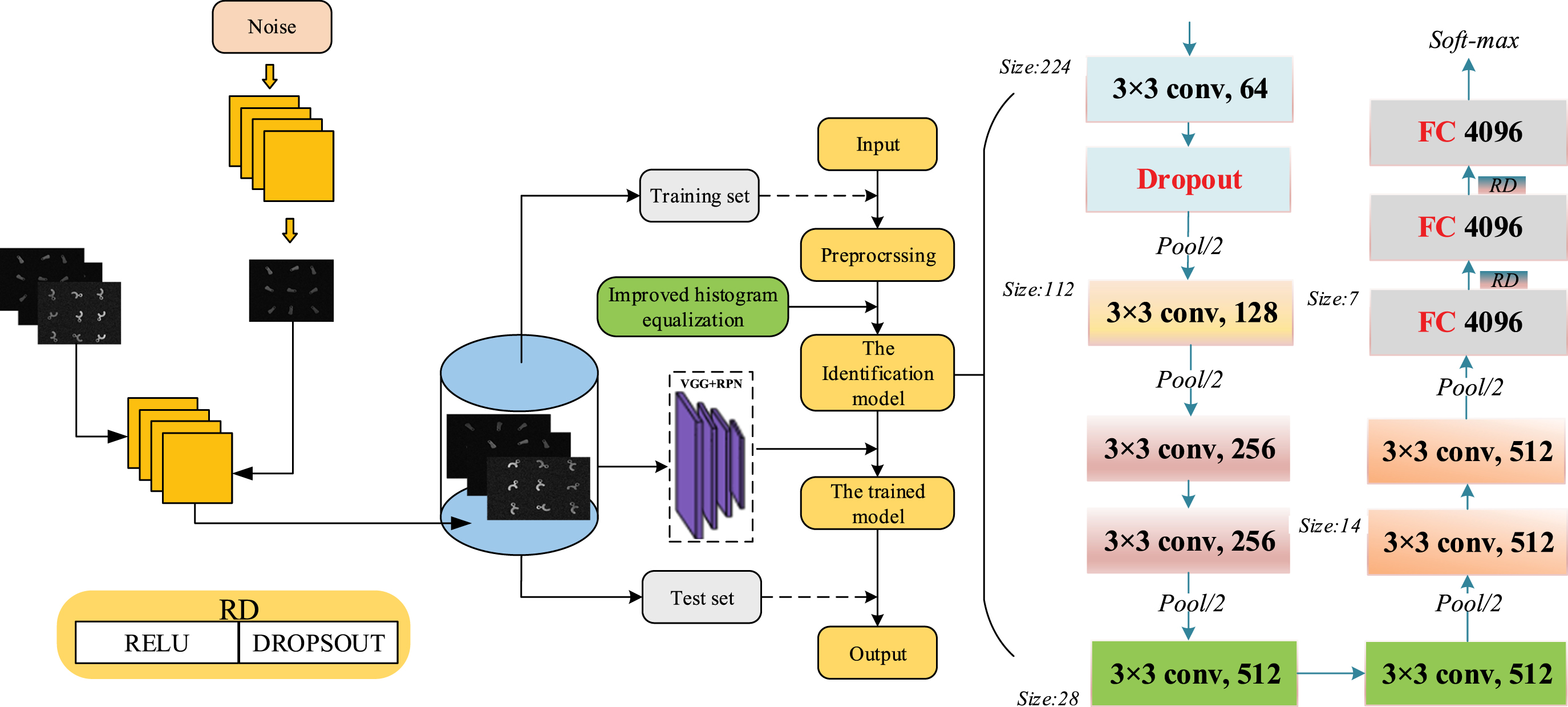
Microoperating system identification flow diagram.

Table 2

The comparison of convolutional neural network performance

Model	Accuracy (%)	Parameters (Million)
This Paper	77.60	15.3
GoogleNet	69.80	6.8
VGG16	78.50	138
LeNet-5	57.20	60
Inception-v3	80.53	23.2

4.2 Microminiature part feature extraction network

Figure 13 a) shows the part map, and 13 b) to f) shows the feature maps from the first layer to the fifth layer, respectively. It can be seen that the smaller targets become more and more blurred with the deepening of the network, which makes it more difficult to identify the tiny parts. On the contrary, the semantic information becomes clearer as the network deepens.

Fig. 13

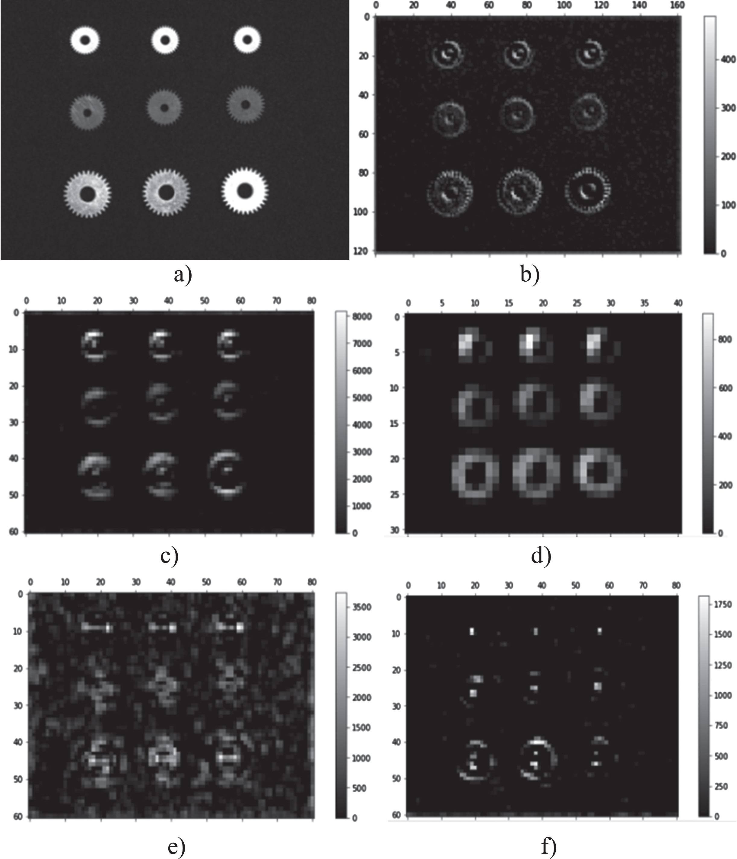
Parts and their characteristic drawings.

To improve the recognition speed of the algorithm, this paper uses depth-level separable convolution for feature extraction, which divides the standard convolution into two convolution operations, depthwise and pointwise. To improve the accuracy of recognition, the fusion of low-level features and high-level features can not only solve the problems of low semantic and much noise of low-level features, but also eliminate the drawbacks of low resolution and poor detail perception of high-level features. Therefore, the second layer features and the fifth layer features are selected for fusion. Figure 14 shows the structure of the feature extraction network and the feature fusion process schematically.

Fig. 14

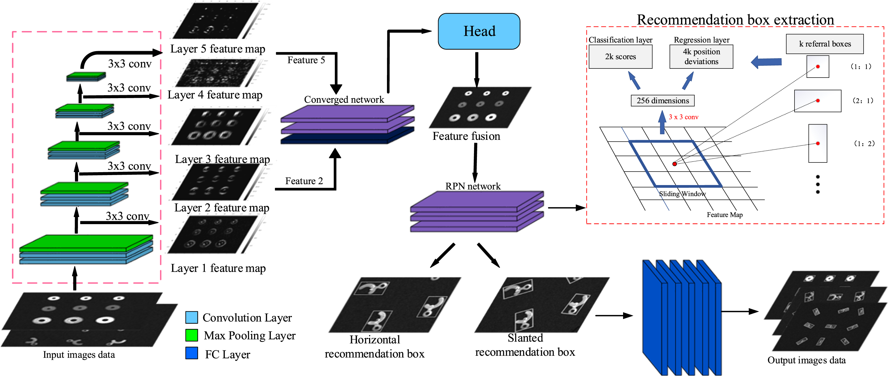
Feature extraction and fusion network framework.

In addition, this paper considers that if the model is trained using the Softmax loss function, when updating the parameters, the model only takes into account the current class and penalizes other classes, thus making the features divisible, but there is no constraint on the intra-class distance, and the final result is that the learned features are divisible, but there is the disadvantage of too large intra-class spacing. In this paper, the central loss function is added to the model training to reduce the problem of large intra-class spacing during classification. The central loss function is defined in the form of the formula: $L_{c} = \frac{1}{2} \sum_{i = 1}^{m} {∥ x_{i} - c_{yi} ∥}_{2}^{2}$ (10)

where: x_i is the input feature and c_yi is the feature center of class i. Where c_yi is defined by Eq:

$Δ c_{j} = \frac{\sum_{i = 1}^{m} δ (y_{i} = j) \cdot (c_{j} - x_{i})}{1 + \sum_{i + 1}^{m} δ (y_{i} = j)}$ (11) swhere: y_i = j in the formula is that c_yi is updated when the categories are the same, and is not updated when the categories are different.

Figure 15 shows the classification of the images before and after adding the central loss function, and the images are reduced to two dimensions for visualization by the data reduction algorithm. Figure 15 a) shows the classification after using the Softmax loss function only, and it can be seen that parts 1–5, although classifiable, are highly susceptible to interference from similar parts, and Fig. 15 b) shows the classification after adding the central loss function. It can be seen that the correlation between different categories becomes smaller after adding the central loss function, which helps to avoid the influence between similar parts when recognizing them.

Fig. 15

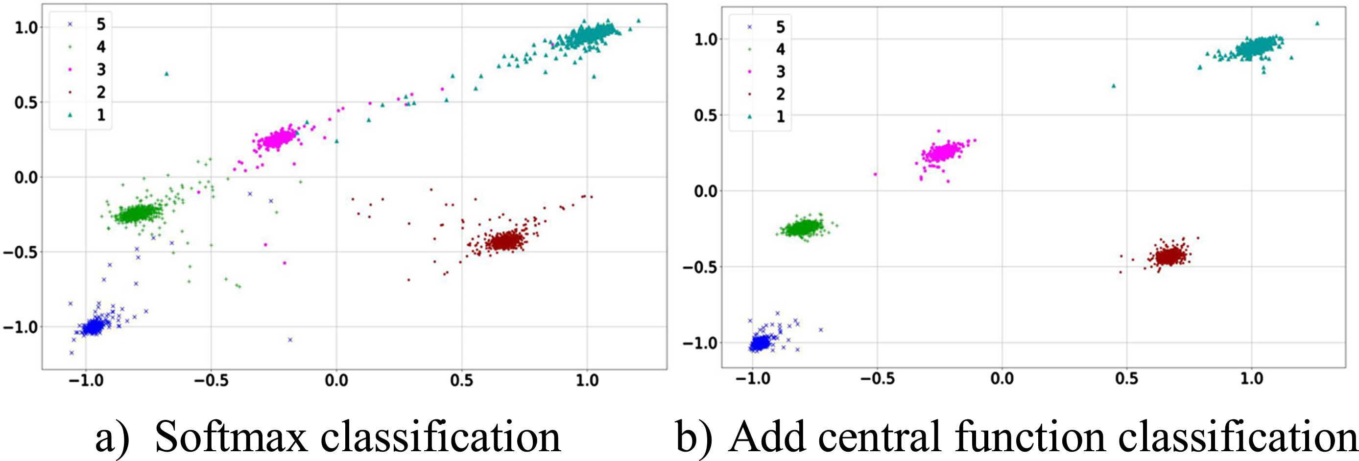
Comparison of loss function results.

5 Model training and test results

5.1 Network model training strategy

In this paper, there are 1400 tiny part datasets, and the training set, validation set, and test set are divided according to the ratio of 6 : 2:2. Among them, the training experiment environment of the model is selected in GPU (NVIDIA Tesla K80 16GB). In the training process although the overall trend of parameter gradient is decreasing, due to the use of small batch training set for parameter update, resulting in parameter gradient oscillation, so there is no guarantee that the network model saved in the training process is optimal. For this reason, this paper saves the model every 100 iterations, the network is iterated for a total of 5000 iterations, and the model weight with the highest accuracy on the validation set is selected as the final model, and the test set is used to verify the performance of the model.

Since the problem to be solved in this paper is the recognition of tiny parts, a small target dataset is used in migration learning. Figure 16 a) shows the training loss vs. test accuracy plot for migration learning. Where curve 1 is the accuracy change of the test set curve 2 is the loss change of the training set, which reaches the saddle point of the loss function when the loss drops to about 0.34 and escapes the saddle point after about 1500 iterations. The parameters of the feature extraction part of the network model have been initialized by migration learning. Figure 16b) shows the training loss and test accuracy curves of the entire network model trained by end-to-end training using the tiny part training set. The network model training effect is good.

Fig. 16

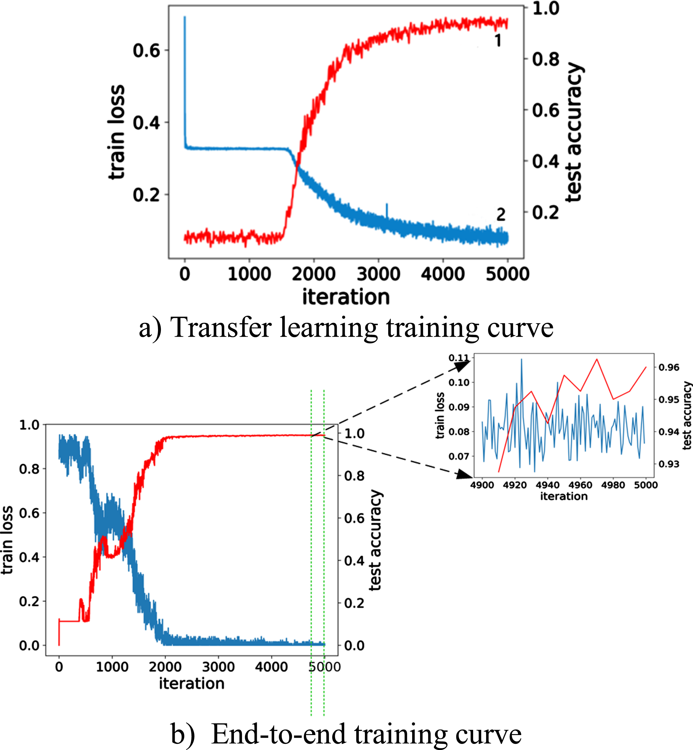
Loss function training change comparison chart.

5.2 Experimental results and analysis

Figure 17 a), b) and c) shows the effect of recognition of five kinds of parts, the rectangular box indicates the position of the part in the image, and the number in the box represents the category of the part. It can be found that the algorithm in this paper can accurately recognize parts with different sizes, different position placements, and different reflection abilities to light.

Fig. 17

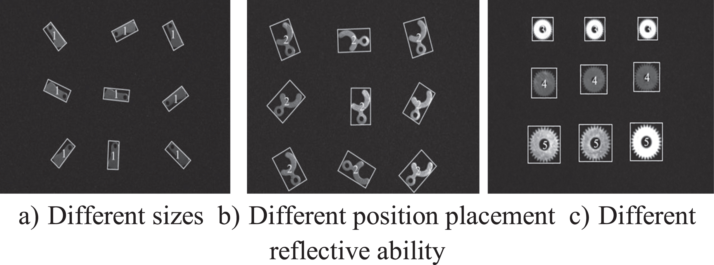
Part distinguish effect drawing.

In part recognition, four cases can occur due to the difference between the algorithm and the actual labels: the sample predicted to be positive is positive (TP), the sample predicted to be positive is negative (FP), the sample predicted to be negative is positive (TN), and the sample predicted to be negative is negative (FN). Precision is generally used as the evaluation criterion of the identification algorithm, and its formula is defined as follows: $Accuracy = \frac{TP}{TP + FP}$ (12)

As can be seen from Equation (12), accuracy is the proportion of samples that are positive among those that are predicted to be positive. Figure 18 shows the comparison chart for the confusion matrix of the recognition algorithm. In this paper, 200 parts were tested, where the numbers on the diagonal of the confusion matrix represent the number of samples predicted to be positive for each type of part that is also positive, and each column represents the number of samples predicted to be positive for each type of part that is negative.

Fig. 18

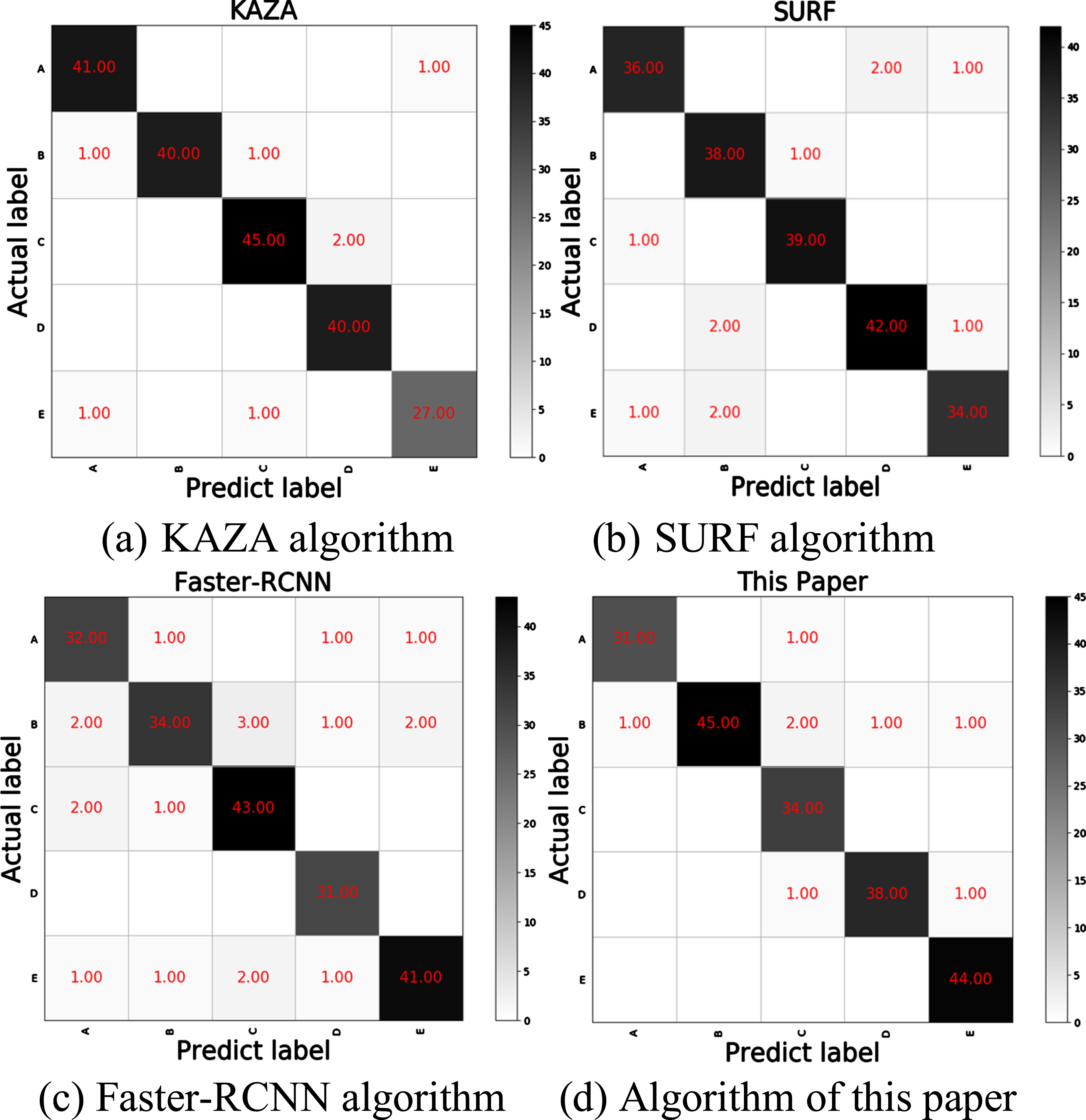
Comparison chart of recognition algorithm confusion matrix.

Table 3 shows the results of the ablation experiments, where V, V-D, F(N/Y), TR(N/Y), and IR(N/Y) denote VGG, VGG-Dropout, whether to replace the activation function, whether to introduce the RPN network, and whether to pass whether to introduce the improved RPN network, respectively. From Table 3, we can see that: the recognition accuracy of the original VGG under the same data set is 78.5%, but the recognition speed is 1.105 s. This indicates that VGG performs poorly for the recognition of tiny parts. B and C are both improvements of the original network structure. From the table B, we can see that when the LRN layer is replaced with Dropout layer, the recognition speed of micro-objects is improved by 0.12 s, which indicates that the network model extracts effective features and enhances the stability of the model. C is the introduction of ReLU activation function on the basis of B, which again enhances the fitting ability of the model. The recognition speed is nearly improved. D introduces the traditional RPN network in VGG on the basis of A, and the recognition speed is 0.42 s. E and F introduce the traditional RPN recommendation frame and the improved RPN recommendation frame on the basis of C, respectively, and the recognition accuracy is 77.3% and 77.9%, respectively. It can be seen that F is the network structure proposed in this paper, and although the recognition accuracy of the network is not optimal, the difference in recognition accuracy is less than 1%, and the recognition speed is more than 1 s higher than that of the traditional VGG network.

Table 3

Results of the ablation experiments with the impoved backone network structure

Method	V-D(N/Y)	F(N/Y)	TR (N/Y)	IR (N/Y)	Recognition Accuracy (%)	Recognition Speed (%)
A. VGG	N	N	N	N	78.5	1.105
B. VGG+D	Y	N	N	N	75.4	1.025
C. VGG+D+R	Y	Y	N	N	76.9	0.586
D. VGG+tRPN	N	N	Y	N	77.2	0.420
E. VGG+D+R+TRPN	Y	Y	Y	N	77.3	0.106
F. VGG+D+R+IRPN	Y	Y	N	Y	77.9	0.015

The accuracy of the four algorithms in recognizing each type of part can be calculated by using Fig. 18. In this paper, the average accuracy of five types of parts is used to compare the algorithms. The average accuracy and speed of the recognition algorithms are compared in Table 4. The average accuracy of the algorithm in this paper is not much different from the KAZA algorithm, but the speed is the fastest among the four algorithms.

Table 4

Comparison of average accuracy and speed of different algorithms

Algorithm	KAZE	SURF	Faster RCNN	This Paper
Average accuracy (%)	96.5	94.5	90.9	95.8
Speed (s)	3.600	1.700	0.100	0.015

6 Discussion

The main object of research in this paper is the use of deep learning algorithms for tiny parts, which provides a new way of thinking about the machine vision tasks involved in industrial manufacturing, and although some progress has been made in terms of recognition efficiency and speed in the study, the following deficiencies exist for a field involving multidisciplinary intersection to be studied next:

This paper mainly introduces the improved convolutional neural network into the recognition of tiny parts, proves the effectiveness of the method, and does not calibrate the parts to obtain the position information in three-dimensional space.

This paper mainly addresses the recognition of tiny parts in the industry, but limited by laboratory materials, only mechanical table parts were studied and achieved significant results, and the next study will be devoted to the task of recognizing tiny parts in more complex situations.

7 Conclusion

In this paper, a new integrated network model, a data enhancement method based on histogram equalization, and an improved image recognition algorithm based on VGG and RPN networks are proposed to accomplish the micro-level part recognition task. The following conclusions can be drawn:

Each sub-block of the histogram equalization is changed during the image pre-processing process, thereby solving the problem of image distortion and background whitening, and generating image data that meets the criteria while facilitating the expansion of the dataset. The results show that the improved histogram equalization method indirectly improves recognition accuracy in terms of distortion removal and contrast compared to traditional image processing.

The improved VGG model is more capable of handling the recognition of tiny parts. The accuracy and recognition speed are selected as indicators to measure the value. The number of parameters of the network in this paper is reduced by up to 80% compared with other networks, but the accuracy is less than 3% different from that of VGG16 and Inception-v3. So the depth-level separable convolution can substantially improve the recognition speed while ensuring accuracy, indicating that the improvement strategy proposed in this paper is effective.

Experimental results supported by several comparison tests show that the improved VGG combined with the RPN network obtains the best classification results, and the improved network model improves in average accuracy by 1.3% and 4.9% compared with SURF and Faster RCNN, respectively. Although there is a 0.7% difference in the average accuracy compared with the KAZE algorithm, the algorithm in this paper improves recognition speed by more than 80% compared with the other three algorithms, and the overall performance is better.

Footnotes

Acknowledgments

This research was funded by National Natural Science Foundation of China, grant number 51975170, the Fundamental Research Foundation for Universities of Heilongjiang Province, grant numberLGYC2018JQ017, the study was supported by Reserve Leader Funding for Leading Talent Echelon of Heilongjiang Province (Innovation and Research Group) and State Key Laboratory of Robotics and Systems (HIT) (SKLRS-2021-KF-13).

Patents

The authors declare that they have no known competing financial interests or personal relationships that could have appeared to influence the work reported in this paper.

Data availability statement

Not applicable

Conflicts of interest

The authors declare no conflict of interest.

References

Chen Qinhan , Yao Lijian , Xu Lijun , Yang Yankun , Xu Taotao , Yang Yuncong and Liu Yu , Horticultural Image Feature Matching Algorithm Based on Improved ORB and LK Optical Flow[J], Remote Sensing 14(18) (2022).

Stange Alexander , Imboden Matthias , Javor Josh , Barrett Lawrence

and Bishop David

, Building a Casimir metrology platform with a commercial MEMS sensor[J], Microsystems & Nanoengineering 5(1) (2019).

Jiayi Ma , Xingyu Jiang , Aoxiang Fan , Junjun Jiang and Junchi Yan , Image Matching from Handcrafted to Deep Features: A Survey[J], International Journal of Computer Vision (2020).

Ye Yuanxin , Shen Li , Hao Ming , Wang Jicheng and Xu Zhu , Robust Optical-to-SAR Image Matching Based on Shape Properties[J], IEEE Geoscience and Remote Sensing Letters 14(4) (2017).

Yanwei Pang , Wei Li , Yuan Yuan and Jing Pan , Fully affine invariant SURF for image matching[J], Neurocomputing 85 (2012).

Hughes Lloyd Haydn , Marcos Diego , Lobry Sylvain , Tuia Devis and Schmitt Michael , A deep learning framework for matching of SAR and optical imagery[J], ISPRS Journal of Photogrammetry and Remote Sensing 169 (2020).

Saqib Hakak , Amirrudin Kamsin , Palaiahnakote Shivakumara , Gulshan amin Gilkar , Wazir Zada Khan and Muhammad Imran , Exact String Matching Algorithms: Survey, Issues, and Future Research Directions[J], IEEE Access 7 (2019).

Dong Zhao , Yan Yang , Zhihang Ji and Xiaopeng Hu , Rapid multimodality registration based on MM-SURF[J], Neurocomputing 131 (2014).

Fan Xiaoyan , Xing Linjie , Chen Jiaxuan , Chen Shuang , Bai Haicheng , Xing Lin , Zhou Chengjiang and Yang Yang , VLSG-SANet: A feature matching algorithm for remote sensing image registration[J], Knowledge-Based Systems 255 (2022).

10.

11.

, Hu

, Northwood

, et al., :Optimization of the electrolytic plasma oxidation processes for corrosion protection of magnesium alloy AM50 using the Taguchi method[J], Journal of Materials Processing Technology 182(1-3) (2007), 58–64.

12.

Ser

P.K.

and Siu

W.C.

, Non-analytic object recognition using the Hough transform with the matching technique[J], IEEE Proceedings-Computers and Digital Techniques 141(1) (1994), 11–20.

13.

Thomas

K.A.

, Joshi

, et al., :Measuring the effect of intimate partner violence on health-related quality of life: a qualitative focus group study[J], Health and Quality of Life Outcomes 5(1) (2007), 67–75.

14.

Kassim

A.A.

, Tan

and Tan

K.H.A.

, Comparative study of efficient generalised Hough transform techniques[J], Image and Vision Computing 17(10) (1999), 737–748.

15.

, Chan

C.W.

and Canters

, Fully Automatic Subpixel Image Registration of Multiangle CHRIS/Proba Data[J], IEEE Transactions on Geoscience and Remote Sensing 48(7) (2010), 2829–2839.

16.

Lowe

D.G.

, Distinctive Image Features from Scale-Invariant Keypoints[J], International Journal of Computer Vision 60(2) (2004), 91–110.

17.

Bay

, Tuytelaars

and Gool

L.V.

, SURF: Speeded Up Robust Features[J], Computer Vision & Image Understanding 110(3) (2006), 404–417.

18.

Alcantarilla

P.F.

, Bartoli

and Davison

A.J.

, KAZE Features[C], Springer Berlin Heidelberg, Springer Berlin Heidelberg, 2012:214–227.

19.

Yang Zhiwei , Numerical approximation and error analysis for Caputo–Hadamard fractional stochastic differential equations[J], Zeitschrift für angewandte Mathematik und Physik 73(6) (2022).

20.

Isozaki Akihiro , Mikami Hideharu , et al., Intelligent image-activated cell sorting 2.0[J], Lab on a Chip 20(13) (2020).

21.

Jang Houk , Liu Chengye , Hinton Henry , Lee Min-Hyun , Kim Haeryong , Seol Minsu , Shin Hyeon-Jin , Park Seongjun and Ham Donhee , An Atomically Thin Optoelectronic Machine Vision Processor[J], Advanced materials (Deerfield Beach, Fla.) 32(36) (2020).

22.

Joseph Redmon , Santosh Divvala , Ross Girshick , et al., You Only Look Once: Unified, Real-Time Object Detection[C], IEEE Conference on Computer Vision and Pattern Recognition (CVPR), Ndonesia: IEEE, 2016:316–320.

23.

Ren

, He

, Girshick

, et al., :Faster R-CNN: Towards Real-Time Object Detection with Region Proposal Networks[J], IEEE Transactions on Pattern Analysis & Machine Intelligence 39(6) (2015), 1137–1149.

24.

, Gkioxari

, Dollar

, et al., Mask R-CNN[J], IEEE (2) (2020).

25.

Linka Kevin and Kuhl Ellen , A new family of Constitutive Artificial Neural Networks towards automated model discovery[J], Computer Methods in Applied Mechanics and Engineering 403(1) (2023).

26.

Lowry

, Sunderhauf

, Newman

, et al., :Visual Place Recognition: A Survey[J], IEEE Transactions on Robotics 32(1) (2016), 1–19.

27.

Masone

and Caputo

, A Survey on Deep Visual Place Recognition[J], IEEE Access 9(9) (2021), 1–10.

28.

Xu Mingjing , Baraldi Piero , Yang Zhe and Zio Enrico , A two-stage estimation method based on Conceptors-aided unsupervised clustering and convolutional neural network classification for the estimation of the degradation level of industrial equipment[J], Expert Systems with Applications 213(55) (2023).

29.

Middya Asif Iqbal , Nag Baibhav and Roy Sarbani , Deep learning based multimodal emotion recognition using model-level fusion of audio–visual modalities[J], Knowledge-Based Systems 244 (2022).

30.

Radjenović-Mrcarica

, Mrcarica

, Detter

and Litovski

, Neural network visual recognition for automation of the microelectromechanical systems assembly[J], International Journal of Neural Systems 8(1) (1997).

31.

Zheng Heliang , Fu Jianlong , Zha Zheng-Jun , Luo Jiebo and Mei Tao , Learning Rich Part Hierarchies with Progressive Attention Networks for Fine-Grained Image Recognition[J], IEEE Transactions on Image Processing: a Publication of the IEEE Signal Processing Society 29 (2019).

32.

Li Jiale , Liu Tao , Wang Xuefei and Yu Jianyou , Automated asphalt pavement damage rate detection based on optimized GA-CNN[J], Automation in Construction 136 (2022).

33.

Zhang Jun , Lu Yaming , Yang Zhe , Zhu Xin , Zheng Ting , Liu Xin , Tian Yaogang and Li Weiguang , Recognition of void defects in airport runways using ground-penetrating radar and shallow CNN[J], Automation in Construction 138 (2022).

34.

Dong

, Wang

, Fang

, Hu

, Zhang

, Ma

, et al., :Innovative Method for Pavement Multiple Damages Segmentation and Measurement by the Road-Seg-CapsNet of Feature Fusion[J], Constr Build Mater 324 (2022), 126719.

35.

Pei

, Sun

, Xiao

, Li

, Sun

and Zhang

, Virtual generation of pavement crack images based on improved deep convolutional generative adversarial network[J], Eng Appl Artif Intel 104 (2021), 104376.

36.

Xia

, Liu

, Xu

and Wang

, Visible-infrared person re-identification with data augmentation via cycle-consistent adversarial network[J], Neurocomputing 443 (2021), 35–46.

37.

Guo

, Jia

, Guo

, Wang

and Zhai

, Retina-inspired in-sensor broadband image preprocessing for accurate recognition via the flexophototronic effect[J], Matter 6(2) (2023).

38.

, Jia

, Tang

, Song

, Liang

, Ren

, Li

, Chen

, Wang

, Lu

, Meng

and Zhu

, Inorganic-Organic Hybrid Phototransistor Array with Enhanced Photogating Effect for Dynamic Near-Infrared Light Sensing and Image Preprocessing[J], Nano Letters (2022).

39.

Zhong

, Wang

, Jin

, Tu

and Luo

, A method of image preprocessing based on nonlinear diffusion and information extraction[J], Computers and Mathematics with Applications 61(8) (2010).

40.

Ravindra Krishna Chandar

and Thangamani

, Suppression of noises using fast independent component analysis (FICA) and signal saturation using fuzzy adaptive histogram equalization (FAHE) for intensive care unit false alarms[J], Measurement 145 (2019).

41.

Li Yiming , Ishitsuka Yuji , Hedde Per Niklas and Nienhaus Ulrich

, Fast and efficient molecule detection in localization-based super-resolution microscopy by parallel adaptive histogram equalization[J], ACS Nano 7(6) (2013).

42.

Martínez Cañada

, Morillas

, Ureña

, Gómez López

J.M.

and Pelayo

F.J.

, Embedded system for contrast enhancement in low-vision[J], Journal of Systems Architecture 59(1) (2013).

43.

Splechtna Rainer , Gracanin Denis , Todorovic Goran , Goja Stanislav , Bedic Boris , Hauser Helwig and Matkovic Kresimir , Interactive Visual Analysis of Structure-borne Noise Data[J], IEEE Transactions on Visualization and Computer Graphics 24 (2022).

44.

Chang

, Wu

, Yang

, Yin

and Luo

, Clustering-based CLEAN algorithm in ghost imaging with sparse spatial frequencies[J], Optics Express 29(23) (2021).

45.

Zhang

, Wei

, Kang

and Li

, Hybrid nonlinear convolution filters for image recognition[J], Applied Intelligence 51(12) (2020).

46.

Shi

, Wang

, Li

and Dou

, Remote Sensing Image Segmentation Based on Hierarchical Student’s-t Mixture Model and Spatial Constrains with Adaptive Smoothing[J], Remote Sensing 15(3) (2023).

47.

Kellil

, Aissat

and Mellit

, Fault diagnosis of photovoltaic modules using deep neural networks and infrared images under Algerian climatic conditions[J], Energy 263(5) (2023).

48.

Hacıefendioğlu Kemal , Başağa Hasan Basri , Yavuz Zafer and Karimi Mohammad Tordi , Intelligent ice detection on wind turbine blades using semantic segmentation and class activation map approaches based on deep learning method[J], Renewable Energy 182 (2022).