Visual SLAM algorithm based on semantic information and geometric consistency 1

Abstract

Localization through intricate traffic scenes poses challenges due to their dynamic, light-variable, and low-textured nature. Existing visual Simultaneous Localization and Mapping (SLAM) methods, which are based on static and texture-rich assumptions, struggle with drift and tracking failures in such complex environments. To address this, we propose a visual SLAM algorithm based on semantic information and geometric consistency in order to solve the above issues and further realize autonomous driving applications in road environments. In dynamic traffic scenes, we employ an object detection network to identify moving objects and further classify them based on geometric consistency as dynamic objects or potential dynamic objects. This method permits us to preserve more reliable static feature points. In low-texture environments, we propose a method that employs key object categories and geometric parameters of static scene objects for object matching between consecutive frames, effectively resolving the problem of tracking failure in such scenarios. We conducted experiments on the KITTI and ApolloScape datasets for autonomous driving and compared them to current representative algorithms. The results indicate that in the dynamic environment of the KITTI dataset, our algorithm improves the compared metrics by an average of 29.68%. In the static environment of the KITTI dataset, our algorithm’s performance is comparable to that of the other compared algorithms. In the complex traffic scenario R11R003 from the ApolloScape dataset, our algorithm improves the compared metrics by an average of 25.27%. These results establish the algorithm’s exceptional localization accuracy in dynamic environments and its robust localization capabilities in environments with low texture. It provides development and support for the implementation of autonomous driving technology applications.

Keywords

Autonomous vehicles SLAM traffic environments object detection

1 Introduction

Localization is a crucial problem in the field of autonomous vehicles, and accurate information enables autonomous driving tasks, such as vehicle control, path planning, and object tracking. Current primary vehicle localization methods include GPS navigation, vision-based localization, LiDAR-based localization, etc. GPS navigation provides all-weather information but does not offer accurate localization information in GPS-denied environments such as urban canyons and tunnels. The LiDAR sensors required for LiDAR-based localization methods are relatively costly, and these methods are not conducive to the implementation of autonomous driving technologies at a low cost. Vision sensors are cheaper and more readily available, for scenarios that require large-scale deployment or limited resources. With the development of artificial intelligence [1, 2] and intelligent electric vehicle technology [3 –5] in recent years, visual Simultaneous Localization and Mapping (SLAM) technology enables real-time modeling and localization functions for scenes using low-cost camera sensors, providing accurate localization information, scene 3D information, and high-precision map information for autonomous vehicles. The development of visual SLAM provides reliable technical support for achieving reliable, safe, and commercialized autonomous driving systems [6, 7].

Vision SLAM algorithms are more adaptable to moving objects in dynamic environments due to the camera’s ability to capture environmental data. It is possible for LiDAR SLAM algorithms to generate errors and necessitate additional processing to deal with dynamic objects. In addition, vision sensors can capture rich color, texture, and shape information, which is beneficial for localization and mapping in low-texture environments. LiDAR sensors may suffer from insufficient geometric information, resulting in degraded performance. Visual SLAM that is based on feature points has been developed relatively well. However, these SLAM systems are unable to maintain sufficient accuracy and robustness in dynamic and low-texture environments, and are even susceptible to failure in challenging scenes. In dynamic environments, dynamic objects in the image violate the data relationships assumed by static SLAM, resulting in inaccurate pose estimation [8]. While the most significant challenge in low-texture environments is the inability to correlate previous frame data with current frame data due to the lack of feature information in images with illumination variations [9].

With the recent development of deep convolutional neural networks, the performance of image-based object detection has improved dramatically, and neural networks can distinguish the pixel space to which the object belongs by acquiring semantic information about the image. Therefore, the combination of deep learning methods and SLAM systems is currently one of the most important development directions. When deep learning is used to replace parts of conventional localization and mapping techniques, it usually starts with feature extraction [10], depth estimation [11, 12], and loop closure detection [13]. This method extracts semantic information from the environment to be added to the mapping, and then improves the accuracy and robustness of localization and mapping with the aid of continuously enriched information and a continuously improved network structure.

There are dynamic and low-texture environments in complex traffic scenes. Moving objects in dynamic environments can disrupt feature point matching and map construction, causing estimated paths and maps to deviate. In addition, areas lacking textures make it difficult for algorithms to precisely match feature points, thereby limiting the accuracy of feature extraction and tracking. Stable and reliable localization results can provide fundamental support for vehicle navigation, path planning, obstacle detection, and map updating, as well as assist autonomous driving systems in sensing the environment and updating environmental information in real-time. However, most SLAM algorithms cannot cope with the above two harsh environments and cannot be used in real traffic scenarios.

We propose an algorithm for visual SLAM based on semantic information and geometric consistency. The algorithm can simultaneously handle feature extraction and tracking in dynamic and low-texture environments, achieving high accuracy and stable localization effects, improving the reliability and adaptability of autonomous driving technology in complex environments, and accelerating the development of autonomous driving technology. In summary, our work has made the following contributions:

We acquire moving objects in traffic scenes using an object detection network with a multi-scale channel attention block and a feature fusion block. In addition, potential moving objects are segmented using semantic information and geometric constraints. While eliminating dynamic features, as many stable features as possible are preserved.

The object detection network is used to detect stationary objects such as traffic signals and signs, to perform feature extraction and screen key objects, to complete the matching of key objects by their categories and geometric parameters, and to perform system initialization and tracking.

A visual SLAM algorithm is proposed for highly variable environments, illumination variations, or complex texture-less scenes. Using the environment’s rich geometric and semantic information and semantic mapping, the algorithm distinguishes between dynamic and stationary objects during tracking and reverts to tracking key objects in the event of tracking failure.

The rest of the paper is organized as follows. Section II discusses related work, Section III describes the framework of our work, and Section IV provides qualitative and quantitative results of visual SLAM on the ApolloScape and KITTI datasets [14, 15]. Finally, Section V provides a brief conclusion, limitations, and discussions. In order to represent the formulas and words in our paper more clearly and unambiguously, the we detail the abbreviations and symbols used and summarize them in a glossary of terms, as shown in Table 1.

Table 1
Glossary of abbreviations and symbols

Symbol/Abreviations Description

E (L) The energy function to be optimized

λ Weight of pairwise energy term

π (•) Projection function

∘ The operator of the 3D transformation

E _i Reprojection error

$T_{w}^{c}$ Camera pose

$W_{k}^{i}$ , $H_{k}^{i}$ Width/Height of the i key object region (pixel)

SLAM Simultaneous localization and mapping

IMU Inertial measurement unit

GC-RANSAC Graph-Cut RANSAC

MSCAB Multi-Scale Channel Attention Block

AFFB Attention Feature Fusion Block

SGD Stochastic Gradient Descent

LM Levenberg-Marquardt

BRIEF Binary Robust Independent Elementary Features

ROS Robot Operating System

ATE Absolute Trajectory Error (m)

Max Maximum error (m)

Mean Mean error (m)

Median Median error (m)

Min Minimum error (m)

RMSE Root Mean Square Error (m)

Symbol/Abreviations	Description
E (L)	The energy function to be optimized
λ	Weight of pairwise energy term
π (•)	Projection function
∘	The operator of the 3D transformation
E _i	Reprojection error
$T_{w}^{c}$	Camera pose
$W_{k}^{i}$ , $H_{k}^{i}$	Width/Height of the i key object region (pixel)
SLAM	Simultaneous localization and mapping
IMU	Inertial measurement unit
GC-RANSAC	Graph-Cut RANSAC
MSCAB	Multi-Scale Channel Attention Block
AFFB	Attention Feature Fusion Block
SGD	Stochastic Gradient Descent
LM	Levenberg-Marquardt
BRIEF	Binary Robust Independent Elementary Features
ROS	Robot Operating System
ATE	Absolute Trajectory Error (m)
Max	Maximum error (m)
Mean	Mean error (m)
Median	Median error (m)
Min	Minimum error (m)
RMSE	Root Mean Square Error (m)

2 Related work

Vision-based localization algorithms have been extensively studied in areas associated with autonomous driving technology, such as dense mapping, object tracking, and semantic segmentation. In this section, we will focus on the portion of the research that addresses the environment with dynamic objects and missing textures and then analyze its problems.

2.1 SLAM in dynamic environments

Currently, most SLAM algorithms assume that the environment is stationary. However, many moving objects, such as vehicles and pedestrians, exist in the real world, and some advanced SLAM algorithms [16] do not perform well in scenes with dynamic objects. In dynamic environments, SLAM algorithms can be divided into two methods, one based on geometry and the other on semantics.

The core idea of the geometry-based method is to distinguish dynamic objects by combining weight functions and motion consistency tests. Wang et al. [17] clustered the depth images and distinguished motion classes based on mathematical models and geometric constraints. Dai et al. [18] separated points belonging to static scenes and different motion objects into different categories based on the correlation between landmarks. Zhang et al. [19] segmented the image region containing the moving object and static background by performing dynamic segmentation on the optical flow estimation result. Although geometry-based methods are faster than semantic-based methods, they are typically less accurate and do not perform well in scenes lacking geometric features.

Semantic information-based methods mainly use neural networks to obtain semantic information about images and distinguish the pixel space to which moving objects belong. Runz et al. [20] proposed MaskFusion for object recognition and segmentation by fusing Mask-RCNN. It improves the boundary accuracy of the object mask using a geometry-based segmentation algorithm to achieve recognition, detection, tracking, and reconstruction of moving rigid bodies. Liu et al. [21] fused Mask-RCNN and PWC-Net for dynamic environments, which used optical flow to predict semantic results in order to acquire more semantic information. Ai et al. [22] proposed a new probabilistic model for dynamic objects based on ORB-SLAM2 and an object detection network to reduce the effect of moving objects on pose estimation and improve the ability to distinguish dynamic objects. Bescosb et al. [23] employed Mask RCNN for segmentation, followed by dynamic object segmentation using a combination of multi-view geometry and deep learning. Yu et al. [24] proposed a SLAM algorithm that incorporated a semantic segmentation network to eliminate the impact of moving people in an indoor environment. Although it performs well in dynamic indoor environments, it is not unsuitable for urban traffic environments. Ganti et al. [25] employed a semantic segmentation network to acquire semantic information about the environment and removed feature points from the corresponding regions of dynamic objects.

Most SLAM algorithms for dynamic environments do not account for the presence of stable, static feature points (e.g., stationary vehicles) in dynamic regions. It may lead to a decrease in the number of points used for tracking, and in some complex environments, localization failures are prone to occur.

2.2 SLAM in low-texture environments

When the texture is missing in a scene due to significant changes in illumination or other factors, the SLAM algorithm based on feature points may experience a severe degradation of pose estimation and localization failure. The SLAM algorithm based on geometric features and object features is currently attracting a great deal of research interest, and it can provide more discriminative localization features and semantic information in environments lacking point features [26].

Yang et al. [27] constructed an object-level SLAM system based on ORB-SLAM2. For stationary object features, the system associates point features with their corresponding high-level features and then matches high-level features in different frames if sufficient point features are present. Nicholson [28] et al. expressed objects as ellipsoids and solved poses using the ellipsoids’ reprojection errors. Tian et al. [29] further refined the initialization of ellipsoids and the data association problem between ellipsoids. However, the method is ineffective in scenes without vehicles. Some approaches [30, 31] represent objects as spheres and use them to correct the scale drift of monocular SLAM. Li et al. [32] combine road structural features to reject dynamic scene feature points. This method improves localization accuracy and robustness, but it performs poorly in scenes where road features are heavily occluded. Xie et al. [33] reprocessed with line features to generate virtual cross-matching points for constructing virtual maps to improve the stability of the visual odometry method in environments with low texture. Some approaches [34, 35] combine IMU (Inertial Measurement Unit) and visual SLAM to improve robustness in low-texture environments, but this issue is not adequately addressed by visual SLAM alone.

Most SLAM algorithms for low-texture environments extract feature points based on geometric features. Therefore, they can’t provide any high-level understanding of the surrounding environment. However, in the SLAM process, it is often desirable to capture and map high-level semantic information about the environment [35]. The information enables intelligent vehicles to distinguish between locations with similar low-level geometric and visual features, enabling advanced driving tasks.

In response to the aforementioned external uncertainties, such as missing or transformed textures, lighting variation, and moving objects, we propose an algorithm based on semantic information and geometric consistency to deal with these uncertainties and enhance the reliability and accuracy of the visual SLAM system.

3 System description

The overview of our SLAM algorithm is shown in Fig. 1. We implemented the SLAM algorithm based on ORB-SLAM3, whereas this paper focuses on the algorithm’s tracking component. The algorithm uses a multi-threaded approach in the tracking part to improve real-time performance. The algorithm performs feature extraction and matching while acquiring potential moving object regions in the traffic environment using deep learning. In addition, the geometric constraint module based on the GC-RANSAC (Graph-Cut RANSAC) algorithm identifies dynamic feature points and preserves stable features. When there are insufficient valid features in the environment due to the missing nearby textures, the algorithm performs pose estimation by tracking and matching key objects in order to improve localization accuracy and stability. After initialization, the system estimates camera poses and optimizes and updates the local mapping’s landmarks.

Fig. 1

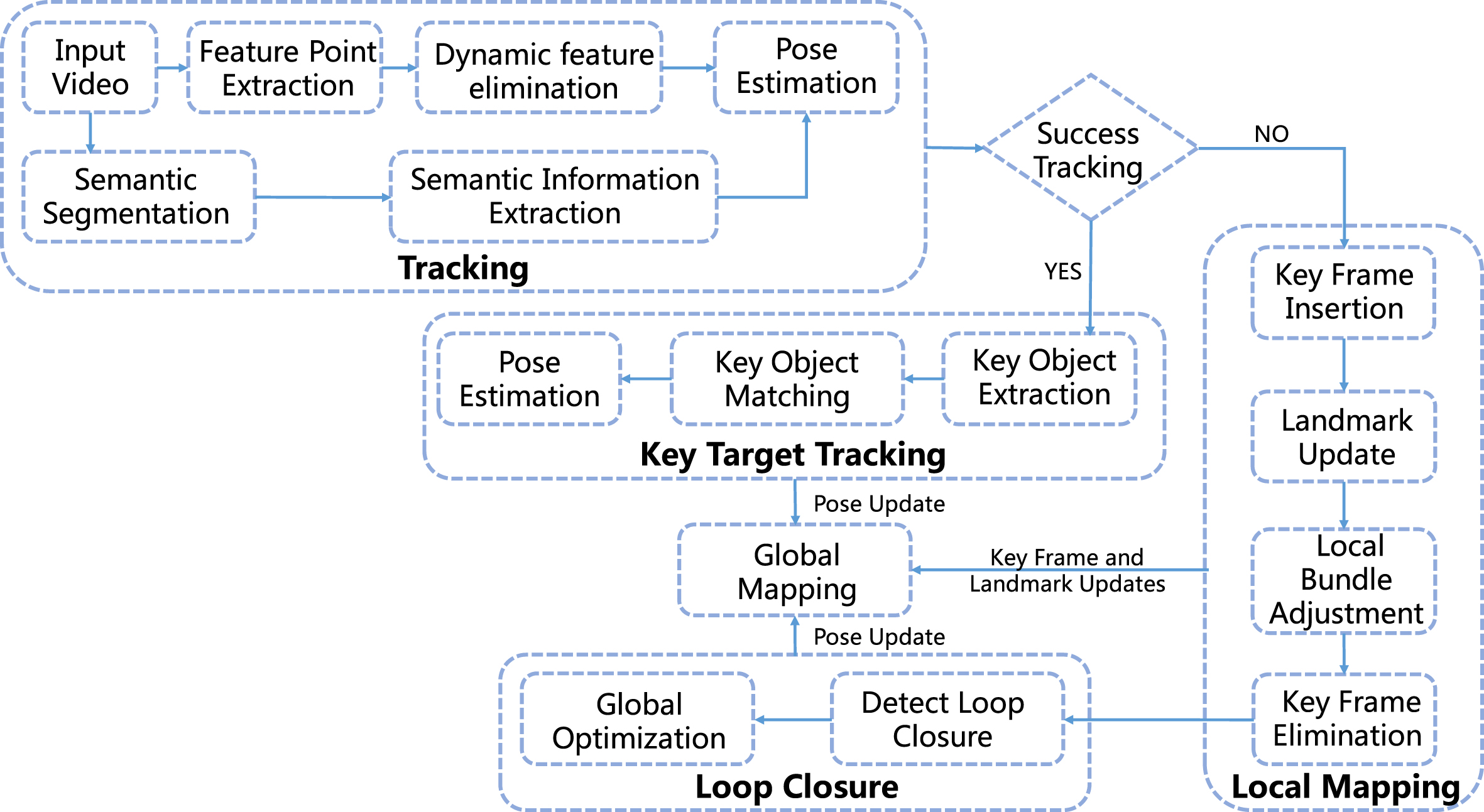
Overview of our SLAM algorithm.

3.1 Semantic module

For the complex traffic scenes with more moving objects, based on the object detection network [37] developed by our group incorporating MSCAB (Multi-Scale Channel Attention Block) and AFFB (Attention Feature Fusion Block) to obtain the semantic information in the environment, the network structure is shown in Fig. 2.

Fig. 2

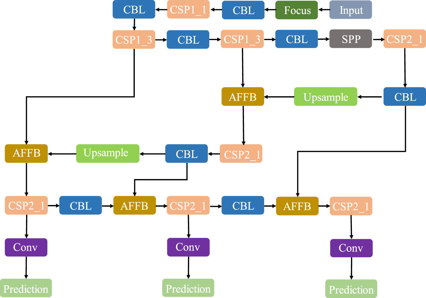
Structure of AFFB_YOLOv5s network.

The BDD100K dataset is primarily used for training the object detection network, while the PASCAL VOC dataset is used as an auxiliary validation dataset. During the preprocessing phase, the JSON tag format of the BDD100K dataset must be converted to the XML tag format of the PAS-CAL VOC dataset before being converted to the txt tag format of the YOLOv5 s dataset. During the training process, we optimize the loss function using the SGD (Stochastic Gradient Descent) algorithm. Then the weight decay coefficient is 0.0005, the initial learning rate is 0.01, the batch size is 32, and the number of epochs is 300. The image input resolution is 640x640. During the testing process, the batch size is 1, and the input image resolution remains at 640×640.

Inspired by ParseNet [38], a 1 × 1 convolution kernel is used to control the scale of local channel attention, resulting in the construction of a multi-scale channel attention block. This block is divided into local and global scales. The global scale uses average pooling to obtain global information, whereas the local scale does not use pooling to retain more detailed information. The multi-scale channel attention module can focus not only on large objects but also on small objects at local scales, thereby enhancing the network’s object detection performance in complex and variable traffic scenes.

To obtain contextual information between different layers, the network combines the attention feature fusion block with the multi-scale channel attention block [37]. A nonlinear fusion scheme is used, and the expression of the output Z ∈ R^C×H×W is as follows: $\begin{matrix} Z = MSCAB (X_{1} \oplus X_{2}) \otimes X_{1} \\ + (1 - MSCAB (X_{1} \oplus X_{2})) \otimes X_{2} \end{matrix}$ (1)

Where MSCAB (X) represents the multiscale channel attention block. Z ∈ R^C×H×W is the output of the attention feature fusion block, and C represents the number of channels of the feature graph. H and Ware the height and width of the feature graph, respectively. X₁ ∈ R^C×H×W and X₂ ∈ R^C×H×W are the two input feature graph, X₁ is the low-level semantic feature graph and X₂ is the high-level semantic feature graph. They represent low-level semantic features and high-level semantic features, respectively. ⊕ represents the addition of broadcasting mechanism, and ⊗ represents elementwise multipication. The fusion weights MSCAB (X₁ ⊕ X₂) and 1 - MSCAB (X₁ ⊕ X₂) both have values between 0 and 1. That allows the network to perform a weighted averaging operation between X₁ and X₂ and to be capable of dynamically learning different levels of semantic information.

The object detection network’s trained semantic categories include ten types of cars, buses, people, bicycles, trucks, motorcycles, trains, riders, traffic signs, and traffic signals. We establish dynamic object categories that include cars, buses, people, bicycles, trucks, motorcycles, trains, and riders based on semantic information.

3.2 Dynamic region detection

3.2.1 Geometric constraint module

Due to the complexity and variability of traffic scenes, it is impossible to determine whether an object is moving or stationary based on its category alone. In addition, removing all feature points in the potentially moving object region will result in a low number of effective feature points and failure in localization. Therefore, we add the object detection network with the geometric constraint-based motion differentiation module to further segment the detected potential motion object regions.

The conventional RANSAC algorithm does not consider the intrinsic connection between feature points when performing the fundamental matrix solution. For an image pair ${I_{i}, I_{i}^{'}}$ with fundamental matrix $F {I_{i}, I_{i}^{'}}$ , the 3D landmark P_i and the matched point pair ${p_{i}, p_{i}^{'}}$ may be static if the matched point pair lies on the epipolar line. Thus, we can use the GC-RANSAC algorithm [39] to formulate the static/dynamic landmark identification problem as inlier/outlier identification during fundamental matrix estimation. For successfully n 2D to 2D matched pairs of feature points $M = {(p_{i}, p_{i}^{'}) | i = 1, . . ., n}$ , the state of each pair marks as an inlier or outlier at each iteration by optimizing the energy function E (L) = ∑ _ iB (L_i) + λ∑ _ (i, j) ∈ GR (L_i, L_j). Where B (L_i) is the unary term of the energy function, R (L_i, L_j) is the pairwise energy term. L = {L_i ∈ {0, 1} |i = 1, . . . n} is the label of the set M, M is the n 2D to 2D matching pairs, and G represents the neighbor graph. λ is the weight.

The unary term of the energy function B (L_i) is formulated as: $B (L_{i}) = {\begin{matrix} K (φ (p_{i}, p_{i}^{'}, θ), ɛ) & L_{i} = 0 \\ 1 - K (φ (p_{i}, p_{i}^{'}, θ), ɛ) & L_{i} = 1 \end{matrix}$ (2)

Where θ is the angular parameter of the fundamental matrix and K (σ, ɛ) = exp(- σ²/(2ɛ²)) is the kernel function. Label L_i = 0 represents the inlier pair and L_i = 1 represents the outlier pair. $φ (p_{i}, p_{i}^{'}, θ)$ is the distance of matching pair $(p_{i}, p_{i}^{'})$ , and ɛ is the threshold for determining the inliers and outliers.

The pairwise energy term R (L_i, L_j) is formulated as: $\begin{matrix} R (L_{i}, L_{j}) = \\ {\begin{matrix} 1 & L_{i} \neq L_{j} \\ (B (L_{i}) + B (L_{j})) / 2 & L_{i} = L_{j} = 0 \\ 1 - (B (L_{i}) + B (L_{j})) / 2 & L_{i} = L_{j} = 1 \end{matrix} \end{matrix}$ (3)

The pairwise energy term penalizes neighboring points whose labeling is inconsistent. For neighbors whose labels are all outliers, the greater their proximity to the model results in a heavier penalty, whereas for neighbors whose labels are all inliers, the greater their proximity to the model results in a lighter penalty.

Feature points from static regions usually originate from fixed objects in the environment and exhibit perspectives, scales, and shapes that are relatively stable. By calculating these relationships between feature points, effective feature matching, and geometric consistency can be achieved. The geometric features of dynamic objects, such as perspectives, scales, and shapes of feature points matched in front and back frames, are not as accurate as those of static objects. Before using the GC-RANSAC algorithm to distinguish between inliers and outliers, count the number of successfully matched feature points $N_{init}^{c}$ in each object region and the number of all successfully matched feature points $N_{init}^{all}$ , and then calculate the proportion $P_{init}^{c}$ of both in the c-th object. After using the GC-RANSAC algorithm to distinguish between inside and outside points, count the number of remaining feature points $N_{last}^{c}$ in each object region and the number of all remaining feature points $N_{last}^{all}$ , and then calculate the proportion $P_{last}^{c}$ of both in the c-th object. The geometric constraint module has two parts [17], the first of which is represented as: $\frac{N_{last}^{c}}{N_{init}^{c}} < \frac{N_{last}^{all}}{N_{init}^{all}} \times T_{reduce}$ (4)

Where T_reduce is the threshold used to distinguish dynamic regions. If the geometric consistency within the object region is poor, the GC-RANSAC algorithm can remove a large number of outliers, and the proportion of remaining inliers will be significantly less than the proportion of all inliers. However, if the object region is too small, too few feature points may exist in this region. In this case, removing a small number of outliers is sufficient to satisfy the aforementioned condition. Therefore, we add the following second part to the geometric constraint module: $P_{init}^{c} > T_{init}$ (5)

Where T_init is a threshold value set for the misclassification of the dynamic region due to the small size of the object regions. Both thresholds are based on references and experimental data results. According to the geometric constraint module described previously, when the c-th object region is determined to be dynamic, the remaining feature points within this object are considered to be outliers and deleted.

The results of detecting dynamic regions using the geometric constraint module in a dynamic environment are shown in Fig. 3. Figure 3(a) depicts a scene with both moving and stationary vehicles. Figure 3(b) depicts a magnified view of the rectangular area following object detection for Fig. 3(a), and 3(c) depicts the mask of the detected moving object region.

Fig. 3

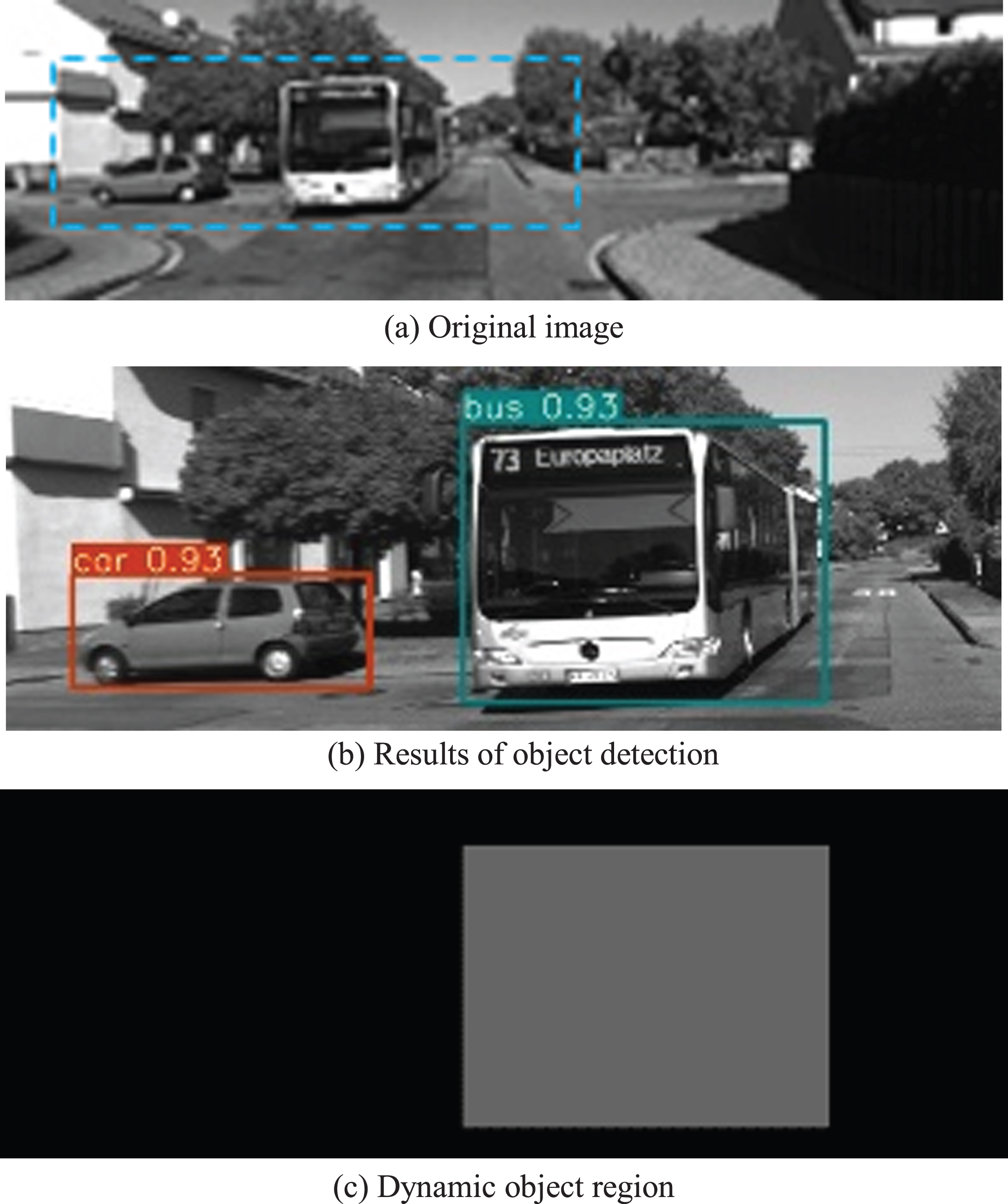
Dynamic region detection in dynamic environment.

The comparison results before and after filtering the feature points are shown in Fig. 4. Then, Fig. 4(a) depicts the original image, Fig. 4(b) illustrates the feature point distribution in the initial state, and Fig. 4(c) shows the remaining feature point distribution after matching filtering. Figure 4(d) depicts the remaining feature point distribution after being filtered by the geometric constraint module, which eliminates all feature points from the moving object region while retaining stable stationary feature points (e.g., parked vehicles on the roadside).

Fig. 4

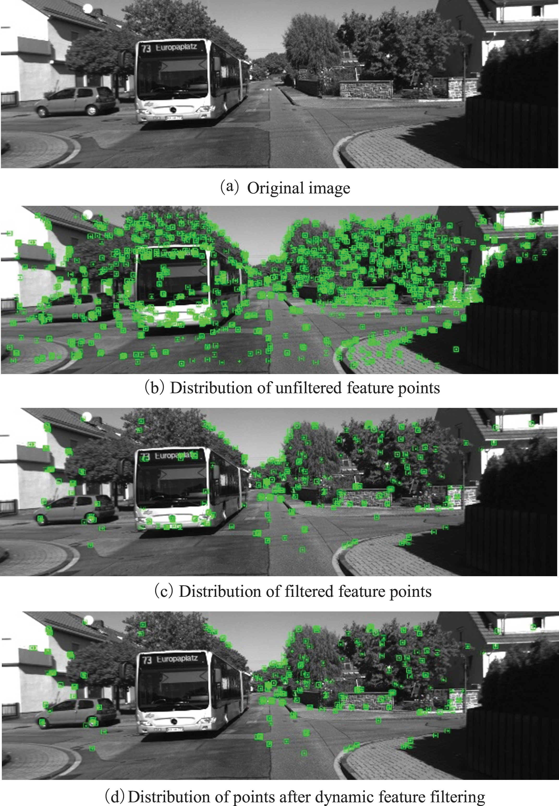
Feature points filtering process.

3.2.2 Pose calculation and optimization module

After removing the feature points corresponding to the dynamic regions, the feature points corresponding to the static regions are utilized for more precise pose estimation. The coordinate of the feature point in the stationary area on the current frame is assumed to be u _ i, its corresponding 3D point position in the world coordinate system is $P_{w}^{i}$ , the reprojection error of the feature point is $E_{i} = u_i - π (T_{w}^{c} \circ P_{w}^{i})$ , and $T_{w}^{c}$ is the camera pose. Camera poses transformation is solved by minimizing reprojection error [40] as follows: $T_{w}^{c} = arg min \sum_i {ρ | | u_i - π (T_{w}^{c} \circ P_{w}^{i}) | |}^{2}$ (6)

Where ρ represents the Huber robust kernel function. It uses Levenberg-Marquardt (LM) optimization method to solve the above equation. We check the reprojection error of every feature points involved in the calculation and remove feature points with higher errors. To improve the accuracy of the pose calculation and the accuracy of the landmarks, the landmarks are extended and filtered, and the coordinates of the 3D points in the local map are optimized locally for BA.

3.3 Key object extraction and tracking module

In the traffic environment, stationary objects such as traffic signals, signs, and billboards are distributed. These objects are rich in textures and have distinctive marking properties. Therefore, these objects are appropriate for feature extraction. When there are insufficient image features, the proposed algorithm uses fixed objects to extract image features. It performs feature matching and pose estimation between successive frames based on the class and geometric parameters of key objects.

3.3.1 System initialization

The module identifies stationary objects in the traffic scene using an object detection network and extracts features from the object region. The number of extracted features is proportional to the area of the object within the image. When a feature point is associated with an object, the module creates an association between the point and the object. Therefore, we consider adding additional constraints, e.g., objects and features should be observed within the 2D bounding box for at least two frames.

We use the quadtree method to homogenize the feature points and avoid excessive bunching of feature points. As shown in Fig. 5, the feature points are relatively evenly distributed across the stationary object detection frame. Then, the number of feature points within the region of the stationary object is used to filter the key objects to ensure that these have sufficient features for subsequent object-based matching and tracking. To complete the construction of objects, the key objects are classified and numbered according to their categories and detection order.

After the completion of key object construction, the system must perform key object matching and initialization as follows:

(1) Key object filtering and matching:

Fig. 5

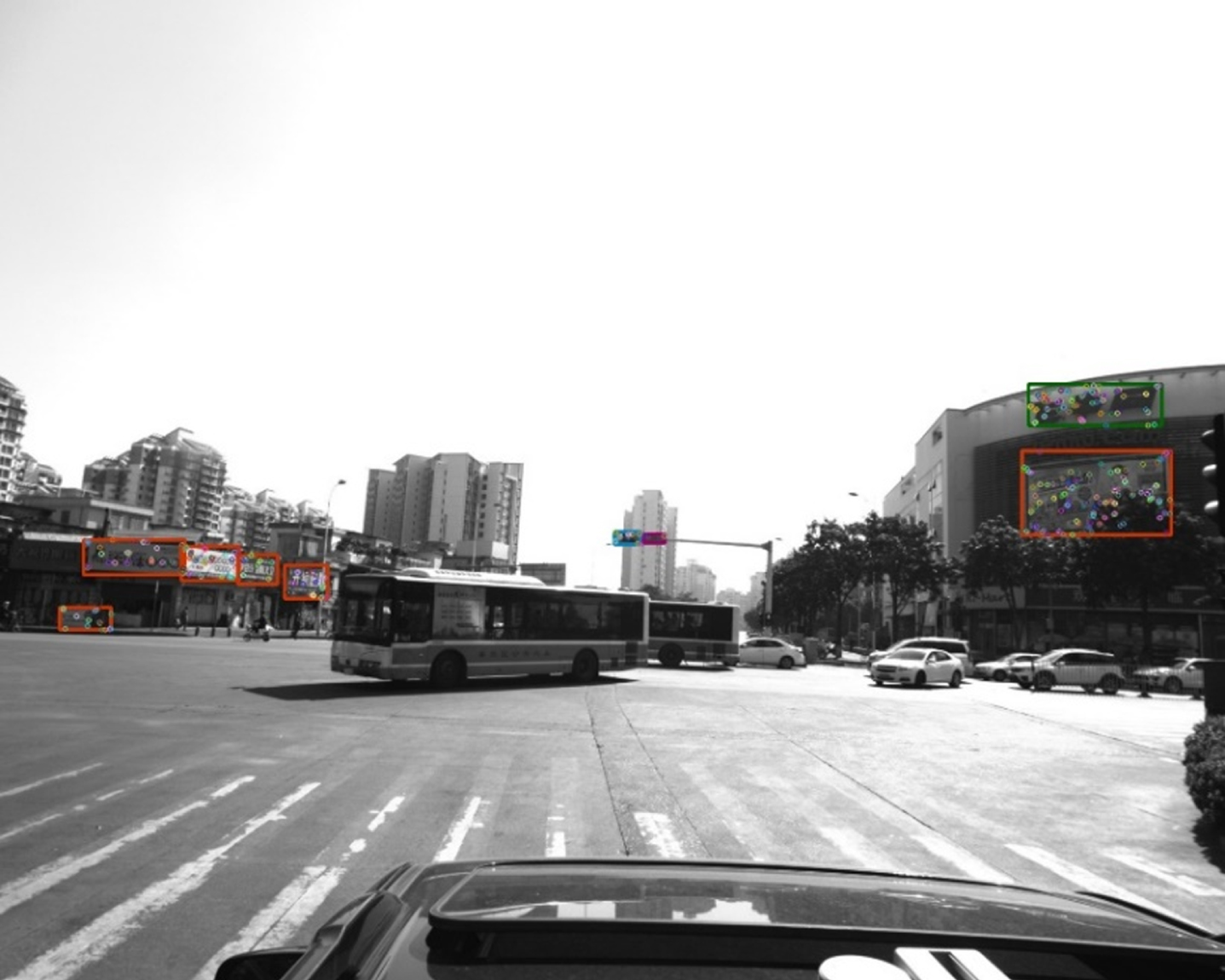
Feature extraction of stationary objects.

Using the center of the key object region as the center of the circle, we establish the matching radius, determine the candidate key objects within the matching radius based on the object category, and filter these candidate objects based on geometric information. The filtering conditions are shown as follows:

$0.75 < \frac{W_{k + 1}^{j} - W_{k}^{i}}{W_{k}^{i}} < 1.25$ (7)

Where $W_{k}^{i}$ is the width of the i key object region to be matched in the previous frame; $W_{k + 1}^{j}$ is the width of the candidate i key object region in the current frame. $0.85 < \frac{H_{k + 1}^{j} - H_{k}^{i}}{H_{k}^{i}} < 1.15$ (8)

Where $H_{k}^{i}$ represents the height of the i key object area to be matched in the previous frame; $H_{k + 1}^{i}$ is the height of the candidate i key object area in the current frame.

When multiple key objects fulfill the geometric filtering conditions, the final filtering is completed by an internal feature association. The filtering method allows the object region’s feature points to be matched sequentially and records the number of successfully matched features. If the number of matching features exceeds the threshold, the matching is deemed successful. Otherwise, the matching fails, and the system removes the object from the current local map. Figure 6 shows the matching results for the key objects, where the two ends of the line correspond to the successfully matched feature points.

(2) Initialization condition

Fig. 6

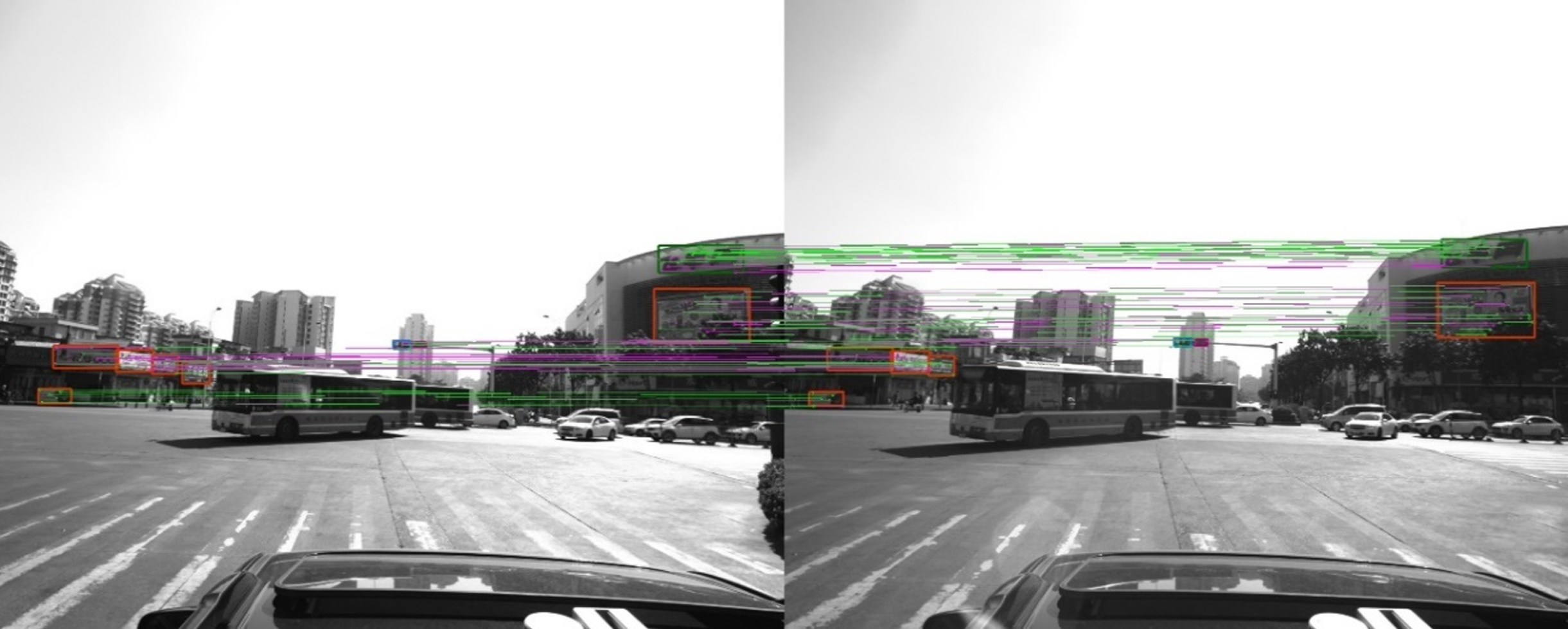
Matching of key objects.

After completing the matching of key objects, the number of successfully matched objects is used to determine whether the initialization condition is satisfied. If the system fulfills the threshold condition, the initialization pose estimation starts. Otherwise, the initialization fails.

(3) Feature pair selection

During the initialization procedure, the RANSAC algorithm is used to randomly select the feature points in two steps. First, we determine the number of key objects, and if there are fewer than eight, we select points in the object area multiple times to ensure that each key object is selected. Then, the specified number of feature points is used to randomly select feature points within a particular key object.

(4) Key object and feature point triangulation

Based on the ratio of feature point triangulation, initialization, and key object area triangulation success is determined. If the object triangulation fails, the key object and all triangulated landmarks within the object are removed.

(5) Initial map construction

After triangulating the key objects, the 3D coordinates of the center of the key objects and the corresponding landmarks are inserted into the map to create the initialized map and establish the foundation for subsequent tracking and camera position calculation based on the key object.

3.3.2 Key object tracking

The pixel coordinates of the center of the key object at the current frame are calculated using the constant velocity model for tracking: $u_{k + 1}^{j} = π (T_{m} \circ P^{j})$ (9)

Where $u_{k + 1}^{j}$ is the image coordinates of the j key object center of the previous frame projected to the current frame; π (•) is the projection function; ∘ is the operator of the 3D transformation of the spatial point coordinates by the positional transformation matrix; T_m is the positional transformation matrix calculated according to the constant velocity model, P^j is the 3D coordinates of the j key object center of the previous frame.

After calculating the location of the key object’s center points, the algorithm sets the search radius and searches the corresponding candidate key object region. Then, it filters by the object category and the geometric information of the object region as the above method.

In order to match key objects with internal feature points, the algorithm determines the search center of the feature point to be matched in the current frame based on the relative pose of the feature points within the key object region. The algorithm searches for feature points within a given radius and selects those with the highest similarity based on the Hamming distance between BRIEF (Binary Robust Independent Elementary Features) descriptors. The algorithm then checks the rotation consistency of the feature points and eliminates those that do not conform to the angle distribution patterns in terms of orientation angle. In addition, it completes the final matching of feature points within the key objects and records the number of successfully matched feature points in each candidate region. The candidate object whose number of features exceeds the threshold is the successfully matched key object. Otherwise, the matching process fails, then those key objects and feature points in the local map are eliminated.

3.3.3 Pose calculation and optimization module

In the low-texture traffic scene, the camera pose transformation is solved based on the object center coordinates and internal feature points after completing the data association between objects: $T_{w}^{c} = arg min \sum_{j = 1}^{n} (E_{po int}^{j} (T_{t}) + E_{center}^{j} (T_{t}))$ (10)

Where T_t ∈ SE (3) represents the current camera pose; $E_{center}^{j}$ is the geometric error at the center point of the key object region, and $E_{po int}^{j} (T_{t}) = \sum_{i = 1}^{m} ρ | | u_{ij} - π (T_{t} \circ P^{ij}) | |^{2}$ consists of the errors of feature points in the j region [40]. P^ij represents the 3D coordinates corresponding to the i feature within the j key object. The algorithm completes the creation of the keyframes. Subsequently, in the local mapping thread, the algorithm jointly optimizes the keyframe poses and key objects according to the LM method.

4 Experimental results

To validate the effectiveness and robustness of the proposed algorithm in complex traffic environments, we evaluate it on the KITTI and ApolloScape autonomous driving dataset with dynamic and low-textured environmental sequences and compare the experimental results with representative SLAM systems [23 , 41,42] from the past few years. The comparison between our work and conventional works is shown in Table 2. We utilized a desktop computer with a 2.90 GHz AMD Ryzen7 4800 H CPU and 16GB of RAM; the system is implemented based on ROS (Robot Operating System) and Ubuntu.

Table 2
Comparison of different methods

Algorithm Deep Learning Dynamic Objects Removal Key Objects Selection Tracking

ORB-SLAM3 – – – √

DynaSLAM √ √ – √

MVSLAM √ √ – √

Ours √ √ √ √

Algorithm	Deep Learning	Dynamic Objects Removal	Key Objects Selection	Tracking
ORB-SLAM3	–	–	–	√
DynaSLAM	√	√	–	√
MVSLAM	√	√	–	√
Ours	√	√	√	√

4.1 Evaluation of algorithms in dynamic environments

The scene containing more dynamic objects in the ApolloScape dataset is verified. A typical scene from this dataset, Road11, is selected as an example, which has 100 frames of images, and it is shown in Fig. 7. The scene has a high proportion of vehicles but few textures in the close area.

Fig. 7

Dynamic scenes in the ApolloScape.

The comparison results of the trajectory experiments in this scene are shown in Fig. 8. Based on the trajectory of ORB-SLAM3 in Fig. 8(a), it is not consistent with the real trajectory change trend, indicating that ORB-SLAM3 has a problem with insufficient robustness in scenes with more dynamic objects. In contrast, DynaSLAM and the proposed algorithm are con-sistent with the ground truth and avoid the problem of unstable localization. From the local enlargement in Fig. 8(b), it can be seen that the error of our algorithm at the end of the trajectory is only 0.2 m, whereas DynaSLAM reaches 0.7 m. This demonstrates that the proposed algorithm can still guarantee stability and accuracy of localization even when there are too many dynamic objects.

Fig. 8

Comparison of plane trajectory.

The performance of our algorithm in this scenario is evaluated using ATE (Absolute Trajectory Error), and the results are displayed in Table 3. ATE is a metric used to evaluate the accuracy of trajectory estimation algorithms by measuring the absolute difference between the estimated trajectory and the actual trajectory. It can be analyzed using a variety of metrics, such as the maximum error, mean error, median error, minimum error, and RMSE (Root Mean Square Error). In this scenario, ORB-SLAM3 has a problem with localization instability, and our algorithm clearly outperforms ORB-SLAM3. Compared to DynaSLAM, our algorithm improves the error maximum, mean, median, and RMSE by 61.64%, 57.07%, 62.36%, and 55.69%, respectively.

Table 3

Comparison of ATE (m) in the dynamic scene from ApolloScape

Algorithm	Max	Mean	Median	Min	RMSE
ORB-SLAM3	17.08	6.503	5.419	1.839	7.669
DynaSLAM	0.5977	0.1570	0.1541	0.0084	0.1837
Ours	0.2293	0.0674	0.0580	0.0157	0.0814

Next, we select a typical dynamic scene from the KITTI dataset for validation; this scene is shown in Fig. 9. Both Figs. 9(a) and (b) depict both moving and stationary vehicles.

Fig. 9

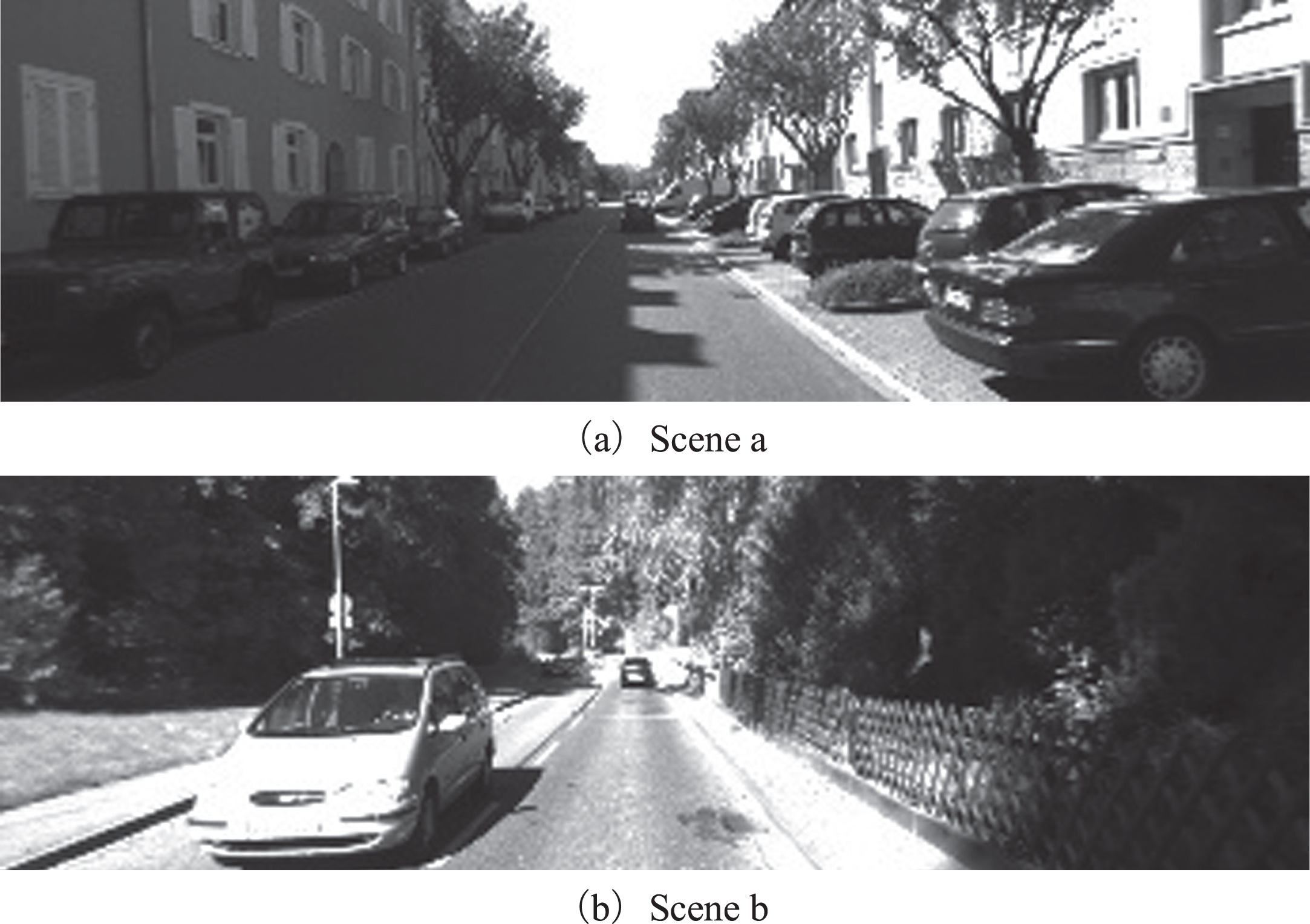
Dynamic scenes in KITTI.

The results of the performance evaluation on the KITTI dataset are shown in Table 4. In scene (a), our algorithm improves the error maximum, mean, median, and RMSE by 20.12%, 20.43%, 21.77%, and 21.97% when compared to DynaSLAM. Compared to ORB-SLAM3, our algorithm improves 11.01%, 12.40%, 12.92%, and 3.85%. Compared to MVSLAM, our algorithm improves 51.41%, 64.58%, 60.74%, and 60.81%. In scene (b), our algorithm improves the error maximum, mean, median, and RMSE by 25.11%, 34.29%, 39.22%, and 32.23%, respectively, when compared to DynaSLAM. Compared to ORB-SLAM3, our algorithm improves by 34.58%, 42.41%, 46.67%, and 41.04%, respectively. Our algorithm outperforms MVSLAM by 33.54%, 8.05%, 5.38%, and 7.59%.

Table 4

Comparison of ATE (m) in the dynamic scene from KITTI

Scene	Algorithm	Max	Mean	Median	Min	RMSE
Scene a	DynaSLAM	0.4775	0.2638	0.2912	0.0002	0.3030
	ORB-SLAM3	0.4286	0.2395	0.2616	0.0002	0.2751
	MVSLAM	0.7850	0.5926	0.5804	0.0444	0.6038
	Ours	0.3814	0.2099	0.2278	0.0002	0.2366
Scene b	DynaSLAM	0.7187	0.3234	0.2952	0.0004	0.3937
	ORB-SLAM3	0.8227	0.3690	0.3364	0.0004	0.4525
	MVSLAM	0.8098	0.2311	0.1896	0.0247	0.2887
	Ours	0.5382	0.2125	0.1794	0.0004	0.2668

Based on the motion differentiation module with geometric constraints, the proposed algorithm subdivides the motion states of the objects. To further demonstrate the effect of retaining static region features on localization precision, we conducted experiments in a scene containing only stationary objects, as shown in Fig. 10. Both Scenes (c) and (d) contain parked vehicles on both sides of the road.

Fig. 10

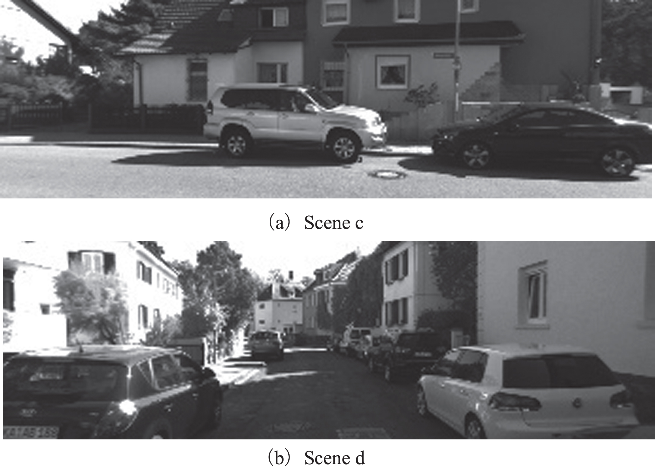
Static scenes in KITTI.

Table 5 shows the performance evaluation results in the above typical static scenes. In scene (c), the proposed algorithm outperforms DynaSLAM by 38.92%, 42.44%, 50.93%, and 44.30% in terms of maximum error, median error, mean error, and RMSE. In scene (d), the proposed algorithm improves the error maximum, median, mean, and RMSE by 20.45%, 22.26%, 11.61%, and 23.22%, respectively, when compared to DynaSLAM. In scenes (c) and (d), our algorithm’s performance is equivalent to ORB-SLAM3 and MVSLAM. Compared to eliminating all feature points on moving objects, experimental results in static scenes indicate that retaining stationary features on potentially moving objects can reduce localization errors.

Table 5

Comparison of ATE (m) in static scenes from KITTI

Scene	Algorithm	Max	Mean	Median	Min	RMSE
Scene c	DynaSLAM	0.2084	0.1072	0.1186	0.0003	0.1246
	ORB-SLAM3	0.1081	0.0623	0.0673	0.0003	0.0685
	MVSLAM	0.1697	0.0550	0.0428	0.0243	0.0648
	Ours	0.1273	0.0617	0.0582	0.0003	0.0694
Scene d	DynaSLAM	0.2430	0.1330	0.1352	0.0005	0.1546
	ORB-SLAM3	0.1900	0.1020	0.1142	0.0005	0.1168
	MVSLAM	0.2485	0.0805	0.0706	0.0177	0.0969
	Ours	0.1933	0.1034	0.1195	0.0005	0.1187

4.2 Evaluation of algorithms in low-texture environments

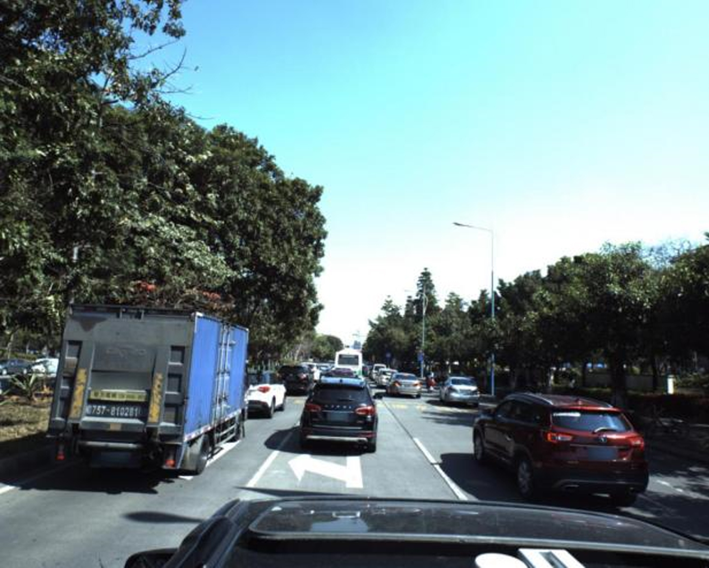
To verify the effectiveness in a near scene with sparse textures, we select a typical low-texture scene from ApolloScape’s Road11 and Road12 for testing, as shown in Fig. 11. In scene (e), due to the intense external illumination and the reflection of the ground, the near-surface loses texture features. The vehicles are in front of moving vehicles in scene (f). In addition, the road surface is heavily obscured and unsuitable for road feature extraction.

In the low-texture scene depicted above, both ORB-SLAM3 and DynaSLAM algorithms experience localization failure, whereas the proposed algorithm successfully completes tracking and has robust localization. A comparison of the trajectory of our proposed algorithm with the ground truth trajectory is shown in Fig. 12.

Fig. 11

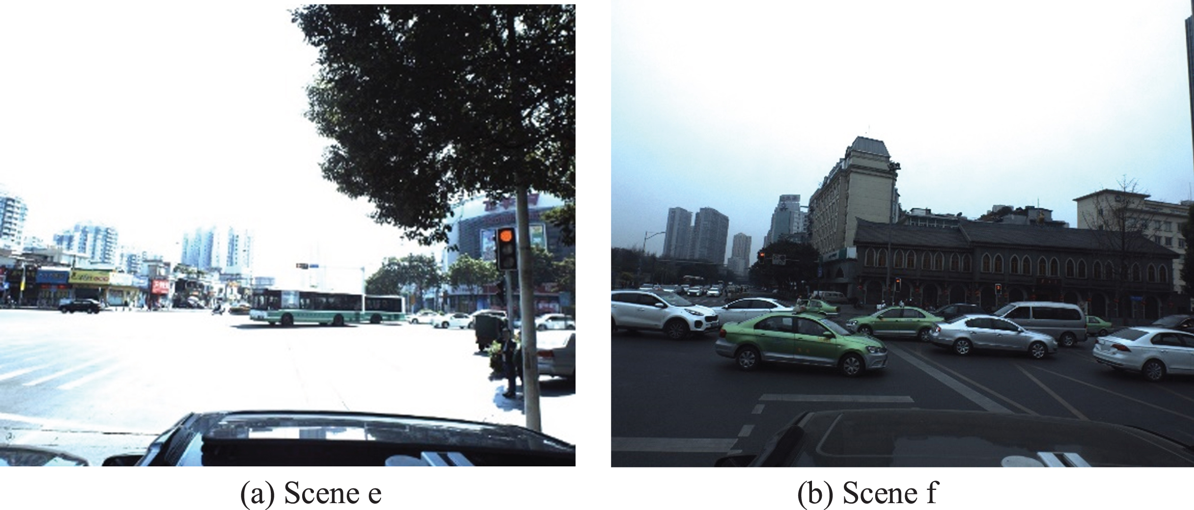
Low-texture scenes in ApolloScape.

Fig. 12

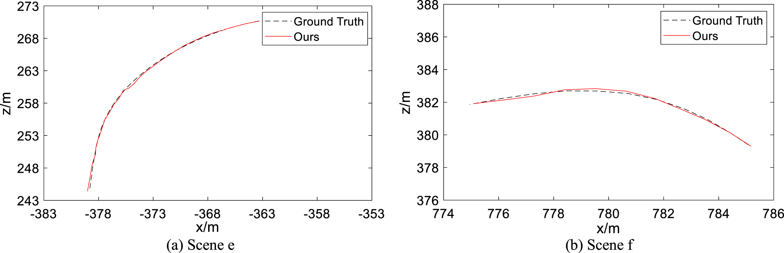
Comparison of plane trajectory.

Experiments conducted on the above typical scene with missing textures demonstrate that our algorithm can effectively perform the localization task in complex environments by identifying key objects and feature points. The trajectory of our algorithm is consistent with the ground truth trajectory and has high localization robustness. We employ ATE as the evaluation index for localization precision, and Table 6 displays the results. The “–” symbol in the table indicates that the algorithm fails to locate this scene and, therefore, cannot determine the trajectory error. Our algorithm prevents localization failure while maintaining a low absolute trajectory error, which satisfies the lane-level localization accuracy requirements for autonomous vehicles.

Table 6

Comparison of ATE (m) in low-texture scenes from ApolloScape

Scene	Algorithm	Max	Mean	Median	Min	RMSE
Scene e	ORB-SLAM3	–	–	–	–	–
	DynaSLAM	–	–	–	–	–
	Ours	0.707	0.228	0.179	0.0692	0.282
Scene f	ORB-SLAM3	–	–	–	–	–
	DynaSLAM	–	–	–	–	–
	Ours	0.169	0.119	0.137	0.0464	0.125

4.3 Evaluation in complex environments

For evaluation purposes, we select consecutive sequences from the ApolloScape dataset. The sequence names of the dataset are abbreviated. For example, the notation for Road11/Record001 is R01R001. Among all the experimental sequences, R11R002 and R11R004 are too short; thus, we abandon them; R11R001 and R12R001 are the most challenging sequences, including scenes with many moving vehicles and few textures. R11R005 is the longest, including 805 frames of images, with a total length of more than 800 m; R11R003 is the shortest, containing 246 images, and the overall distance is approximately 300 m.

As shown in Fig. 13, R11R001 and R12R001, ORB-SLAM3 and DynaSLAM fail to track in the most complex sequence of traffic scenes, whereas our algorithm succeeds. The trajectory of our algorithm overlaps with the ground truth, indicating the effectiveness of the localization algorithm.

Fig. 13

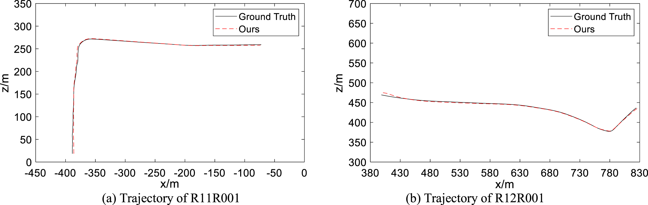
Comparison of plane trajectory.

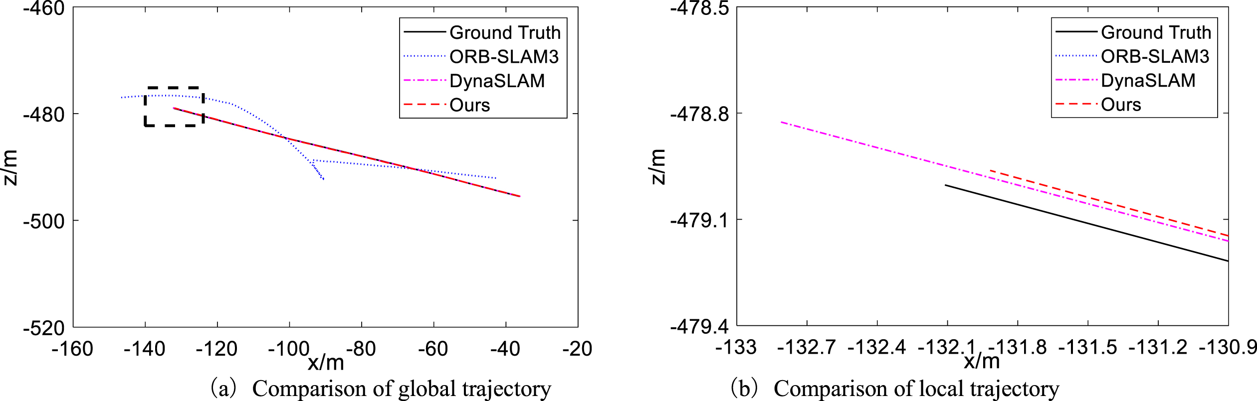
The plane trajectories of R11R003, R11R005, and R11R006 are shown in Fig. 14, with the left side representing the global trajectory and the right side representing the magnified local trajectory in the rectangular box. From Fig. 14(a), the end of the trajectory of our algorithm differs from the ground truth by about 0.5 m, while ORB-SLAM3 and DynaSLAM differ by about 1.4 m and 1.0 m, respectively. In R11R006, the error at the end of our algorithm’s trajectory differs from the ground truth trajectory by approximately 1.6 m, while the error at the end of DynaSLAM’s trajectory differs from the ground truth trajectory by approximately 3.7 m. In addition, the differences between the three algorithms at the end of the trajectory are relatively significant, as shown in Fig. 14(b). The difference between our algorithm and the ground truth trajectory is about 5.8 m, while the differences between ORB-SLAM3 and DynaSLAM are about 8.4 m and 9.9 m, respectively.

Fig. 14

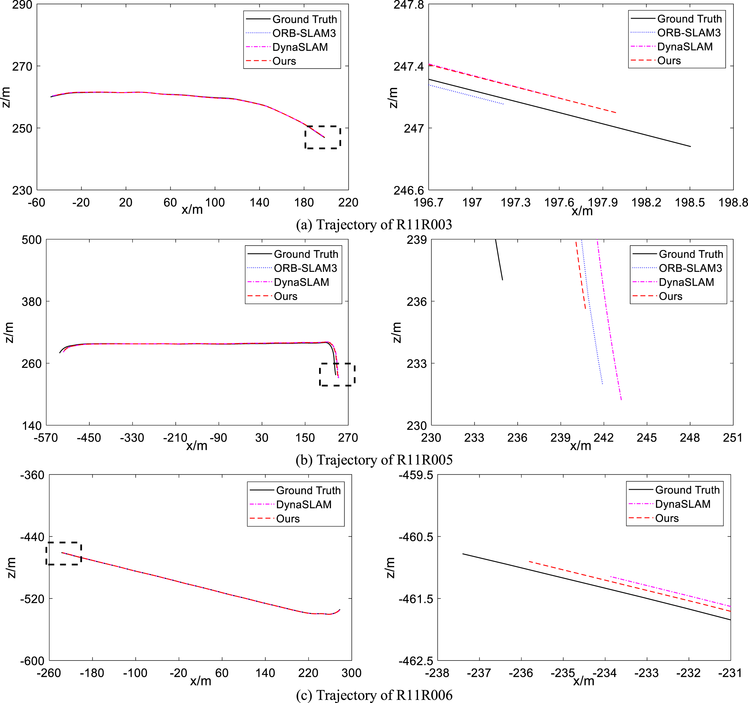
Comparison of plane trajectory.

We employ ATE as the evaluation index based on Table 7 results. In addition, in the extremely challenging R11R001, R11R006, and R12R001 sequences, ORB-SLAM3 and DynaSLAM experience localization failure, whereas the proposed algorithm maintains high localization accuracy while preventing failure. In the R11R003, R11R005, and R11R007 sequence scenarios, our algorithm outperforms the competing algorithms in terms of overall performance. In particular, for the R11R3 sequence, our algorithm improves on five metrics by 34.25%, 41.07%, 34.97%, 3.28%, and 43.10% over ORB-SLAM3, and by 3.19%, 25%, 22.38%, 19.18%, and 26.28% over DynaSLAM. Based on the above analyses, our algorithm has greater localization accuracy and stability in complex traffic scenes than ORB-SLAM3 and DynaSLAM.

Table 7

Comparison of ATE (m) in complex traffic scenes

Sequences	Algorithm	Max	Mean	Median	Min	RMSE
R11R001	ORB-SLAM3	–	–	–	–	–
	DynaSLAM	–	–	–	–	–
	Ours	2.507	1.356	1.380	0.543	1.427
R11R003	ORB-SLAM3	1.708	0.616	0.592	0.061	0.710
	DynaSLAM	1.160	0.484	0.496	0.073	0.548
	Ours	1.123	0.363	0.385	0.059	0.404
R11R005	ORB-SLAM3	9.709	3.721	3.708	0.288	4.326
	DynaSLAM	10.875	4.382	4.308	0.290	5.037
	Ours	8.977	3.576	3.535	0.275	4.140
R11R006	ORB-SLAM3	–	–	–	–	–
	DynaSLAM	3.553	1.104	1.046	0.050	1.318
	Ours	3.769	0.693	0.637	0.0527	0.878
R11R007	ORB-SLAM3	8.588	2.398	2.203	0.027	2.894
	DynaSLAM	6.597	2.537	2.501	0.063	2.996
	Ours	5.947	2.354	2.293	0.086	2.754
R12R001	ORB-SLAM3	–	–	–	–	–
	DynaSLAM	–	–	–	–	–
	Ours	7.304	1.506	1.378	0.634	1.795

To determine the effectiveness of various algorithms, we experiment with the average execution time of our algorithm, DynaSLAM, and ORB-SLAM3. Table 8 shows the results. Our algorithm integrates semantic and geometric modules, but due to the multi-threaded acceleration of the semantic information extraction part and feature point extraction and matching part, the average time per frame is increased by 39.66 ms compared to ORB-SLAM3 and the processing speed reaches 10.8 Fps. Therefore, the algorithm can still satisfy the real-time requirement. DynaSLAM, on the other hand, uses instance segmentation and does not utilize multi-threading for acceleration, resulting in significantly lower efficiency and a running time of 964.78 ms per frame, which is insufficient to meet the real-time requirements.

Table 8

Runtime evaluation (ms)

Algorithm	Semantic module	Geometric module	Tracking
ORB-SLAM3	–	–	53.19
DynaSLAM	911.68	–	964.78
Ours	65.36	17.54	92.85

5 Conclusions and future work

We propose a visual SLAM algorithm for complex traffic scenes in highly dynamic and low-texture environments that is based on semantic information and geometric consistency. Experimental results indicate that, in the dynamic environment of the KIT-TI dataset, the algorithm presented in this paper outperforms DynaSLAM, ORB-SLAM3, and MVSLAM by an average of 26.89%, 25.62%, and 36.52%, respectively, in each metric of ATE. In the static environment of the KITTI dataset, the proposed algorithm’s performance in each metric of ATE is comparable to that of the other compared algorithms. In complex traffic scenario R11R003, compared to DynaSLAM and ORB-SLAM3, the proposed algorithm improves each ATE metric by an average of 19.21% and 31.33%, respectively. In complex traffic scenarios R11R001, R11R006, and R12R001, the compared algorithms fail to localize, whereas our algorithm can reliably and robustly output localization results. In summary, our algorithm improves the robustness and precision of autonomous driving systems in complex and variable traffic environments, providing foundations and providing support for the commercialization of driverless driving applications.

Our proposed visual SLAM, which is based on semantic and geometric constraints, can perform accurate and reliable localization in real-time, but it has limitations. It relies on a depth model for object detection for the initial extraction of moving objects, which may result in inaccurate environment modeling in unfamiliar and non-typical scenarios, thereby affecting the algorithm’s accuracy and reliability. Secondly, due to the limitations of onboard hardware devices and sensor noise, real-time applications may necessitate large-scale maps and increase the system’s computational efficiency and storage requirements. In addition, our proposed method employs a single sensor and does not combine data from additional sensors. In extremely harsh environments, the algorithm’s robustness may not be as good as the multi-sensor fusion approach. Finally, SLAM based on semantic information focuses more on geometric and visual features, cannot take advantage of all the semantic information in the environment, and inaccurate semantic labels have a tendency to introduce errors in mapping and localization. Future research will focus on improving the model’s detection and generalization capability in complex traffic road scenarios, combining static and semantic maps to deal with dynamic environments, and fusing multi-sensor heterogeneous data to improve the accuracy and stability of localization in harsh environments.

References

Tutsoy

, COVID-19 epidemic and opening of the schools: Artificial intelligence-based long-term adaptive policy making to control the pandemic diseases[J], Ieee Access 9 (2021), 68461–68471.

Ad-Hoc, Mobile, and Wireless Networks: 18th International Conference on Ad-Hoc Networks and Wireless, ADHOC-NOW 2019, Luxembourg, Luxembourg, October 1–3, 2019, Proceedings[M], Springer Nature, 2019.

Vanchinathan

, Valluvan

K.R.

, Gnanavel

et al. Numerical simulation and experimental verification of fractional-order PI λ controller for solar PV fed sensorless brushless DC motor using whale optimization algorithm[J], Electric Power Components and Systems 50(1-2) (2022), 64–80.

Vanchinathan

and Selvaganesan

, Adaptive fractional order PID controller tuning for brushless DC motor using artificial bee colony algorithm[J], Results in Control and Optimization 4 (2021), 100032.

Vanchinathan

and Valluvan

K.R.

, A metaheuristic optimization approach for tuning of fractional-order PID controller for speed control of sensorless BLDC motor[J], Journal of Circuits, Systems and Computers 27(08) (2018), 1850123.

Wang

, Hu

, Scherer

Tartanvo: A generalizable learning-based vo[J], arXiv preprint arXiv:2011.00359, 2020.

, Rong

and Wu

, A survey: which features are required for dynamic visual simultaneous localization and mapping?[J], Visual Computing for Industry, Biomedicine, and Art 4(1) (2021), 1–16.

Liu

and Miura

, RDS-SLAM: real-time dynamic SLAM using semantic segmentation methods[J], Ieee Access 9 (2021), 23772–23785.

Qin

, Chen

et al. Avp-slam: Semantic visual mapping and localization for autonomous vehicles in the parking lot[C], 2020 IEEE/RSJ International Conference on Intelligent Robots and Systems (IROS), IEEE, 2020:5939–5945

10.

Tang

, Ericson

, Folkesson

et al. GCNv2: Efficient correspondence prediction for real-time SLAM[J], IEEE Robotics and Automation Letters 4(4) (2019), 3505–3512.

11.

Teed

and Deng

, Droid-slam: Deep visual slam for monocular, stereo, and rgb-d cameras[J], Advances in Neural Information Processing Systems 34 (2021), 16558–16569.

12.

Zhao

, Sun

, Zhang

et al. Monocular depth estimation based on deep learning: An overview[J], Science China Technological Sciences 63(9) (2020), 1612–1627.

13.

Dong

, Qin

, Chang

et al. Weighted triplet loss based on deep neural networks for loop closure detection in VSLAM[J], Computer Communications 186 (2022), 153–165.

14.

Huang

X.Y.

, Wang

, Cheng

X.J.

et al. The ApolloScape Open Dataset for Autonomous Driving and its Application[J], IEEE Transactions on Pattern Analysis and Machine Intelligence 42(10) (2020), 2702–2719.

15.

Geiger

, Lenz

, Stiller

et al.Vision meets robotics: the KITTI dataset[J], The International Journal of Robotics Research 2 (2013), 1231–1237.

16.

Mur-Artal

and Tardós

J.D.

, Orb-slam2: An open-source slam system for monocular, stereo, and rgb-d cameras[J], IEEE Transactions on Robotics 33(5) (2017), 1255–1262.

17.

Wang

, Wan

, Wang

et al. A new RGB-D SLAM method with moving object detection for dynamic indoor scenes[J], Remote Sensing 11(10) (2019), 1143.

18.

Dai

, Zhang

, Li

et al. Rgb-d slam in dynamic environments using point correlations[J], IEEE Transactions on Pattern Analysis and Machine Intelligence 44(1) (2020), 373–389.

19.

Zhang

, Zhang

, Li

et al. Flowfusion: Dynamic dense rgb-d slam based on optical flow[C], 2020 IEEE International Conference on Robotics and Automation (ICRA), IEEE, 2020:7322–7328.

20.

Runz

, Buffier

, Agapito

MaskFusion: Real-Time Recognition, Tracking and Reconstruction of Multiple Moving Objects[C], 2018 IEEE International Symposium on Mixed and Augmented Reality (ISMAR), Munich, Germany: 2018:2018:10–20.

21.

Liu

and Miura

, RDMO-SLAM: Real-time visual SLAM for dynamic environments using semantic label prediction with optical flow[J], Ieee Access 9 (2021), 106981–106997.

22.

, Rui

, Yang

et al. Visual SLAM in dynamic environments based on object detection[J], Defence Technology 17(5) (2021), 1712–1721.

23.

Bescos

, Facil

J.M.

, Civera

et al. DynaSLAM: tracking, mapping and Inpainting in dynamic scenes[J], IEEE Robotics and Automation Letters 3(4) (2018), 4076–4083.

24.

, Liu

X.J.

et al. DS-SLAM: A semantic visual SLAM towards dynamic environments[C], 2018 IEEE/RSJ International Conference on Intelligent Robots and Systems (IROS), IEEE, 2018:1168–1174.

25.

Ganti

, Waslander

S.L.

Network uncertainty informed semantic feature selection for visual SLAM[C], 2019 16th Conference on Computer and Robot Vision (CRV), IEEE, 2019:121–128.

26.

Liang

and Wang

, A Semi-Direct Monocular Visual SLAM Algorithm in Complex Environments[J], Robotic Systems 101(1) (2021), 1–19.

27.

Yang

and Scherer

, Cubeslam: Monocular 3-d object slam[J], IEEE Transactions on Robotics 35(4) (2019), 925–938.

28.

Nicholson

, Milford

and Sünderhauf

, Quadricslam: Dual quadrics from object detections as landmarks in object-oriented slam[J], IEEE Robotics and Automation Letters 4(1) (2018), 1–8.

29.

Tian

, Zhang

, Feng

et al. Accurate and robust object SLAM with 3D quadric landmark reconstruction in outdoors[J], IEEE Robotics and Automation Letters 7(2) (2021), 1534–1541.

30.

Frost

, Prisacariu

and Murray

, Recovering stable scale in monocular SLAM using object-supplemented bundle adjustment[J], IEEE Transactions on Robotics 34(3) (2018), 736–747.

31.

Sucar

, Hayet

J.B.

Bayesian scale estimation for monocular slam based on generic object detection for correcting scale drift[C], 2018 IEEE International Conference on Robotics and Automation (ICRA), IEEE, 2018:5152–5158.

32.

Li Linhui , Zhang Xitong , Lian Jing et al. Semantic SLAM algorithm combined with road structured features[J], Journal of Harbin Institute of Technology 53(2) (2021), 175–183.

33.

Xie

, Yang

, Ning

et al. A Monocular Visual Odometry Method Based on Virtual-Real Hybrid Map in Low-Texture Outdoor Environment[J], Sensors 21(10) (2021), 3394.

34.

Kayhani

, Zhao

, McCabe

et al. Tag-based visual-inertial localization of unmanned aerial vehicles in indoor construction environments using an on-manifold extended Kalman filter[J], Automation in Construction 135 (2022), 104112.

35.

Yang

, Wang

, Liu

et al. An Improved Monocular PL-SlAM Method with Point-Line Feature Fusion under Low-Texture Environment[C], 2021 4th International Conference on Control and Computer Vision, 2021:119–125.

36.

Qian

, Patath

, Fu

et al. Semantic slam with autonomous object-level data association[C], 2021 IEEE International Conference on Robotics and Automation (ICRA), IEEE, 2021:11203–11209

37.

Yin Yuhang Research on Object Detection Method in Traffic Scenes Based on Feature Fusion [D], Dalian: Dalian University of Technology, 2021.

38.

Dai

, Gieseke

, Oehmcke

et al. Attentional Feature Fusion[C], IEEE Winter Coference on Applications of Computer Vision, Online: IEEE, 2021: 3560–3569.

39.

Z.J.

, Huang

S.S.

, Mu

T.J.

et al. Accurate dynamic SLAM using CRF-based long-term consistency[J], IEEE Transactions on Visualization and Computer Graphics 28(4) (2020), 1745–1757.

40.

Bao

, Komatsu

, Miyagusuku

et al. Stereo camera visual SLAM with hierarchical masking and motion-state classification at outdoor construction sites containing large dynamic objects[J], Advanced Robotics 35(3-4) (2021), 228–241.

41.

Campos

, Elvira

, Rodriguez

J.J.

et al. ORB-SLAM3: An Accurate Open-Source Library for Visual, Visual-Inertial, and Multimap SLAM[J], IEEE Transactions on Robotics 37(6) (2021), 1874–1890.

42.

Dong

, Xu

, Wu

et al. Pair-navi: Peer-to-peer indoor navigation with mobile visual slam[C], IEEE INFOCOM 2019-IEEE Conference on Computer Communications IEEE, 2019:1189–1197.

Visual SLAM algorithm based on semantic information and geometric consistency 1

Abstract

Keywords

1 Introduction

2.1 SLAM in dynamic environments

2.2 SLAM in low-texture environments

3 System description

3.2.1 Geometric constraint module

3.3.1 System initialization

Table 2 Comparison of different methods Algorithm Deep Learning Dynamic Objects Removal Key Objects Selection Tracking ORB-SLAM3 – – – √ DynaSLAM √ √ – √ MVSLAM √ √ – √ Ours √ √ √ √

References

Table 2
Comparison of different methods

Algorithm Deep Learning Dynamic Objects Removal Key Objects Selection Tracking

ORB-SLAM3 – – – √

DynaSLAM √ √ – √

MVSLAM √ √ – √

Ours √ √ √ √