A parsimonious ensemble with optimal deep learning and secondary decomposition for short-term wind speed forecasting

Abstract

Wind energy needs to be used efficiently, which depends heavily on the accuracy and reliability of wind speed forecasting. However, the volatility and nonlinearity of wind speed make this difficult. In volatility and nonlinearity reduction, we sequentially apply complete ensemble empirical mode decomposition with adaptive noise (CEEMDAN) and variational mode decomposition (VMD) to secondarily decompose the wind speed data. This framework, however, requires effectively modeling multiple uncertainty components. Eliminating this limitation, we integrate crow search algorithm (CSA) with deep belief network (DBN) to generate a unified optimal deep learning system, which not only eliminates the influence of multiple uncertainties, but also only adopts DBN as a predictor to realize parsimonious ensemble. Two experiments demonstrate the superiority of this system.

Keywords

Parsimonious ensemble secondary decomposition optimal deep learning crow search algorithm

Nomenclature

ANN

Artificial neural network

HBSA

Hybrid backtracking search algorithm

EMD

Empirical mode decomposition

EMT

Empirical wavelet transform

SSA

Singular spectrum analysis

BPNN

Back propagation neural network

GRNN

General regression neural network

ENN

Elman neural network

CNN

Convolutional neural network

GWO

Gray wolf optimization

GRU

Gated recurrent unit

DBN

Deep belief network

SVM

Support vector machine

Wavelet transform

EEMD

Ensemble empirical mode decomposition

Wavelet decomposition

IMF

Intrinsic mode function

RBFNN

Radial basis function neural network

WNN

Wavelet neural network

BiLSTM

Bidirectional long short-term memory

Differential evolution

ELM

Extreme learning machine

PSO

Particle swarm optimization

RBM

Restricted Boltzmann machine

1 Introduction

1.1 Background

Renewable energy is indispensable and its importance is increasing. In the case of China, renewable energy represents 20% of main energy consumption [1]. Wind energy is more economically friendly and widely available that can be used for energy conversion to produce electricity than other renewable energy sources. In the future, the application of wind energy will expand. Additionally, the utilization of wind energy is not only a highly significant research area, but also a challenging task. The instability of wind speed may cause various problems in wind power systems. Therefore, precise and reliable wind speed forecasting is essential to assure the stable operation for wind power systems. This study is dedicated to developing a superior system that could efficiently handle the instability of wind speed and realize high accuracy in wind speed modeling and prediction, thereby ensuring the safety and reliability of wind energy applications.

1.2 Literature review

In recent years, researchers have proposed three main approaches to wind speed prediction, which are physical models, statistical models and artificial intelligence-based models. Physical models use meteorological and geographic data to make predictions. However, due to requiring large amounts of data and slow updates, they does not perform well in the area of short-term wind speed forecasting [2]. Compared to physical models, statistical models try to establish a mathematical relationship between the inputs and outputs, and therefore its forecasting accuracy is higher [3], but they have the shortcoming of not being able to detect the nonlinear features of the wind speed sequence. Artificial intelligence-based models, such as ANN [4 –6], SVM [7 –9], and fuzzy logic [10, 11], are the third forecasting methods that have achieved great success in short-term wind speed forecasting. One of them, deep learning, has even outstanding performance and is able to obtain highly accurate prediction results [12 –16]. In addition, deep learning has been applied to other aspects of forecasting such as electricity load [17, 18] and price [19, 20] with great accuracy. Anyway, artificial intelligence-based deep learning is a very ideal choice of prediction model application.

The application of artificial intelligence models is only part of the improvement in prediction accuracy. In many recent studies, data pre-processing techniques have become a powerful tool to handle the non-linear and non-stationary properties of wind speed sequences. When it came to combining artificial intelligence model with data pre-processing techniques, Du et al. utilized CEEMD to decompose the raw wind speed sequence into several subsequences and fed them into the Elman neural network for prediction respectively [21]. Taking advantage of the fact that VMD can eliminate redundant noise in the wind speed signal, Zhang et al. designed a wind speed prediction system consisting of VMD, HBSA, and ELM [22]. To better understand the data schema, the system proposed by Jaseena et al. combined the advantages of both data decomposition methods and BiLSTM network, where data decomposition methods, including WT, EMD, EEMD and EWT, had been applied to denoise the dataset, respectively [23].

Although the application of single decomposition technology combined with artificial intelligence models in time series prediction has been widely realized, there is still much room for improvement in the modeling process since the single decomposition technology always cannot completely handle the non-stationary properties of wind speed sequences, secondary decomposition is one of these ideas. Just as the prediction system developed by Liu et al. also included a secondary decomposition, they utilized firstly WD to decompose the raw wind speed into several subcomponents, and then used VMD to perform a secondary decomposition of the most unpredictable subcomponents [24]. Further, the combination of the secondary decomposition technology and the deep learning algorithm is embodied in the prediction system proposed by Zhang et al. [25]. For the secondary decomposition part, the multivariate EMD was used to decompose the original sequences filtered out the noise by SSA into the respective IMFs and residuals.

There are a variety of methods to handle the subsequences obtained using decomposition technology, and in some studies, the obtained subsequences are chosen to be fed separately into different prediction models. Just like the combination model designed by Zhang et al. [26] based on CEEMDAN and five neural networks, it firstly applied CEEMDAN to divide the raw wind speed signal into several IMFs, then these IMFs were sent to BPNN, RBFNN, GRNN, WNN and ENN respectively for wind speed prediction. This may improve the prediction accuracy to a certain extent, but multiple prediction models will inevitably increase the parameters that need to be adjusted and the complexity of the system, which in turn leads to a decrease in training efficiency, and the weight coefficients of each prediction model are not easy to be determined. To this end, based on the benefits that DBN outperforms most prediction models and is capable of extracting the deep features of the data to accurately establish input-output mapping relationships, we choose to train this individual optimal deep learning to generate a parsimonious ensemble system.

1.3 Our work and contributions

According to the above literature review and analysis, we propose a parsimonious ensemble forecasting system comprising CEEMDAN, VMD, CSA and individual DBN in this study. Firstly, CEEMDAN and VMD are combined as a novel secondary decomposition technology for filtering the noise of raw wind speed sequence. To be specific, the highest frequency component obtained from the CEEMDAN decomposition is processed secondarily by VMD. Then, an optimal deep learning model integrating CSA with DBN for wind speed forecasting is designed, and applying the optimal DBN instead of multiple forecasting models can not only obtain accurate forecasting results, but also make the system less complex thereby improving training efficiency, finally achieve parsimonious ensemble and efficient forecasting.

In general, the novelties and contributions of this research can be summarized below.

For precise and reliable wind speed forecasting, a parsimonious ensemble system integrating novel secondary decomposition technology and optimal deep learning is proposed.

The deep learning model DBN outperforms most forecasting models. Applying it instead of multiple forecasting models to model each subsequence separately, not only can obtain precise forecasting results, but also can reduce the system complexity and thus improve the training efficiency. Ultimately, the system achieves parsimonious ensemble and efficient forecasting.

The combination of CEEMDAN and VMD as a novel secondary decomposition technology is developed to sufficiently attenuate the non-stationarity of wind speed sequences. In particular, the number of subsequences obtained from the decomposition is determined using sample entropy analysis rather than based on empirical judgment, making the decomposition more scientific and accurate.

DBN as a superior deep learning model has a high upper performance limit. Hyperparameters search for DBN using CSA helps it to reach this upper limit and in turn achieves optimal deep learning.

The distribution of the contents of this paper is arranged as follows. Section 2 reviews the CEEMDAN, VMD, DBN, and CSA methods in detail and describes the framework construction process of the developed CEEMDAN-VMD-DBN-CSA model. Section 3 provides a specific analysis of the proposed model and shows some details of the modeling. Section 4 compares the performance of the developed model with several other models in two experiments respectively, and the results are analyzed and discussed in-depth. Finally, Section 5 concludes with a summary of the important achievements of this paper.

2 Methodology and model framework

This section introduces in detail the CEEMDAN, VMD, DBN, CSA and the parsimonious ensemble CEEMDAN-VMD-DBN-CSA model framework built from them. Of these, CEEMDAN is capable of dealing with the volatility of wind speed and is employed to achieve the first-level decomposition of original wind speed series; VMD enables to decompose the complex high-frequency series into several single-component series; DBN as a deep learning model can identify the input-output relationship in various situations; CSA is an intelligent optimization algorithm that finds the optimal hyper-parameters for DBN with its powerful search capability.

2.1 CEEMDAN

CEEMDAN allows less experiments required by adding a limited amount of adaptive Gaussian white noise to each decomposition [27]. Furthermore, CEEMDAN can overcome the mode mixing problem because its decomposition and reconstruction are complete.

Let x denote the original time series, E_k denote the kth mode of EMD, wⁱ denote the zero-mean Gaussian white noise with unit variance (i is the number of trial, i = 1, 2, …, I), and ɛ_k denote the standard deviation of the white noise at each decomposition stage. The implementation steps of CEEMDAN are described below [28 –30].

Step ding172: Add a pair of Gaussian white noise.

$x^{i} = x + ɛ_{0} w^{i}$ (1) where xⁱ denotes the series of the i-th trial, ɛ₀ denotes the standard deviation of the initial Gaussian white noise.

Step ding173: Decomposition using EMD method to obtain the first mode.

${IMF}_{1} = \frac{1}{I} \sum_{i = 1}^{I} {imf}_{1}^{i}$ (2)

Step ding174: Calculate the first residual.

$r_{1} = x - {IMF}_{1}$ (3)

Step ding175: Calculate the k-th residual.

$r_{k} = r_{(k - 1)} - {IMF}_{k}, k = 2, 3, \dots, K$ (4)

Step ding176: Decompose the residual with added Gaussian white noise to obtain the (k + 1)-th mode of CEEMDAN.

${IMF}_{(k + 1)} = \frac{1}{I} \sum_{i = 1}^{I} E_{1} (r_{k} + ɛ_{k} E_{k} (w^{i}))$ (5)

Step ding177: Repeat steps 4-5 until all IMFs are gained. The final residual R can be expressed as:

$R = x - \sum_{k = 1}^{K} {IMF}_{k}$ (6)

2.2 VMD

VMD, as a time-frequency analysis approach, is capable of decomposing a multi-component sequence into multiple single-component amplitude modulated sequences at one time. It decomposes the raw sequence into the specified amount components by constructing and solving a constrained variational problem. Suppose f denotes the raw sequence and K denotes the number of components, the corresponding expression for the constraint variation is listed below [31, 32].

${\begin{matrix} min_{u_{k}, w_{k}} {\sum_{k} {∥ \partial (t) [(δ (t) + \frac{j}{π t}) * u_{k} (t)] e^{- {jw}_{k} t} ∥}_{2}^{2}} \\ s . t . \sum_{k} u_{k} = f \end{matrix}$ (7) where δ(t) is Dirac distribution and * is convolution operation. And u_k and w_k denote the kth mode component and the corresponding central frequency, respectively.

Next, the Lagrangian multiplier λ(t) is introduced into Equation (7) and the constrained variational problem will be transformed into an unconstrained variational problem [33]. The corresponding augmented expression is given below.

$\begin{matrix} L ({u_{k}}, {w_{k}}, {λ}) \\ = α \sum_{k} {∥ \partial (t) [(δ (t) + \frac{j}{π t}) * u_{k} (t)] e^{- {jw}_{k} t} ∥}_{2}^{2} \\ + {∥ f (t) - \sum_{k} u_{k} (t) ∥}_{2}^{2} \\ + 〈 λ (t), f (t) - \sum_{k} u_{k} (t) 〉 \end{matrix}$ (8) where α is a quadratic penalty factor. And the alternate direction method of multipliers (ADMM) [34] is used to search for saddle points and solve the unconstrained variational problem, where u_k, w_k and λ are updated by the equations below:

${\hat{u}}_{k}^{n + 1} (w) = \frac{\hat{f} (w) - \sum_{i \neq k} {\hat{u}}_{i} (w) + \frac{\hat{λ} (w)}{2}}{1 + 2 α {(w - w_{k})}^{2}}$ (9)

$w_{k}^{n + 1} = \frac{f_{0}^{\infty} w {| {\hat{u}}_{k}^{n + 1} (w) |}^{2} dw}{f_{0}^{\infty} {| {\hat{u}}_{k}^{n + 1} (w) |}^{2} dw}$ (10)

${\hat{λ}}^{n + 1} (w) = {\hat{λ}}^{n} (w) + τ [\hat{f} (w) - \sum_{k} {\hat{u}}_{k}^{n + 1} (w)]$ (11) where w denotes frequency, $\hat{f} (w), {\hat{u}}_{i} (w), \hat{λ} (w)$ denote the Fourier transform of f (t) , u_i (t) , λ (t) respectively, and τ denotes the update step.

Summarizing the above description, Fig. 1 displays the flowchart of VMD.

Fig. 1

The flowchart of VMD.

2.3 Details on DBN

DBN has been extensively applied to classification, feature learning and collaborative filtering [35] since it was originally proposed by Hinton [36], and it contains unsupervised learning sub-part RBM and the logistic regression layer BP neural network for prediction. This subsection introduces the structure of DBN.

2.3.1 RBM

RBM is a random neural network that learns the distribution on its input set. The network usually consists of a visible layer and a hidden layer, with bidirectional full connectivity between neurons in the visible and hidden layers, and no connectivity between neurons of the same layer [37]. Figure 2 illustrates the specific structure of RBM.

Fig. 2

The structure of RBM.

The learning process of RBM is implemented by an energy function. Given visible layer unit v_k, hidden layer unit h_j and its connection weight W_j,k, bias a_k for v_k and b_j for h_j, the energy function E (v, h) for a certain state can be expressed as [38]:

$\begin{matrix} E (v, h) = - \sum_{k = 1}^{n_{v}} a_{k} v_{k} \\ - \sum_{j = 1}^{n_{h}} b_{j} h_{j} - \sum_{k = 1}^{n_{v}} \sum_{j = 1}^{n_{h}} h_{j} W_{j, k} v_{k} \end{matrix}$ (12)

Then, the energy function defines the probability distribution P (v, h) on the visible and hidden layers as:

$P (v, h) = e^{- E (v, h)} / Z$ (13)

$Z = \sum_{v} \sum_{h} e^{- E (v, h)}$ (14) where Z is the partition function.

Knowing all neurons v in the visible layer, the probability that the hidden layer neuron h_j is activated is:

$P (h_{j} = 1 | v) = sigm (b_{j} + \sum_{k = 1}^{n_{v}} W_{j, k} v_{k})$ (15) where sigm (·) is the activation function.

Similarly, knowing all neurons h in the hidden layer, the probability that the visible layer neuron v_k is activated is:

$P (v_{k} = 1 | h) = sigm (a_{k} + \sum_{j = 1}^{n_{h}} W_{j, k} h_{j})$ (16)

The RBM is trained to minimize the energy function, and the contrast divergence (CD) [39] is an effective method to train the RBM by which a one-step Gibbs sampling approximation can be obtained. Figure 3 illustrates the learning process for one iteration.

Fig. 3

The training process of RBM.

After a group of iteration, the modified values for the connection weights and bias are calculated according to the following equation.

$\begin{array}{l} Δ W_{j, k} = η (〈 v_{k} h_{j} 〉 - 〈 {v^{'}}_{k} {h^{'}}_{j} 〉) \\ Δ a_{k} = η (〈 v_{k} 〉 - 〈 {v^{'}}_{k} 〉) \\ Δ b_{j} = η (〈 h_{j} 〉 - 〈 {h^{'}}_{j} 〉) \end{array}$ (17) where η denotes the learning rate and < >denotes the mathematical expectation of the variable.

2.3.2 BPNN

BPNN is a feedforward network trained according to the gradient descent algorithm, which continuously adjusts the weights and biases by back propagating the error to minimize the loss function of the network [40].

The mean square error is calculated as:

$E = \frac{1}{T} \sum_{t = 1}^{T} {(y_{t} - {\bar{y}}_{t})}^{2}$ (18) where y_t, ${\bar{y}}_{t}$ and T are the actual value, predicted value and sample size, respectively.

Then the weight is updated as:

$w^{'} = w - α \frac{\partial E}{\partial w}$ (19) where α is the learning rate.

2.3.3 DBN

DBN is constructed by stacking RBM layer by layer and adding a logistic regression layer BPNN at the end of the stack. The structure of DBN is shown in Fig. 4. The training process of the whole DBN consists of two main stages: the RBM for pre-training and the BPNN for backward fine-tuning.

Fig. 4

The structure of DBN.

First, the initial weights of the network are pre-trained using the unsupervised learning method of RBM, where each RBM is trained individually layer by layer. Specifically, the hidden layer of the former RBM will be connected in the network as the visible layer of the latter RBM.

Next, BPNN receives the output of the last RBM and fine-tunes the entire network with the method of back-propagation error [41].

2.4 CSA

As one of the most intelligent birds, crows pay attention to where other birds hide their food when they are hiding it, in order to steal it after they leave. In fact, crows predict the behavior of burglars based on their own stealing experience as a way to determine the safest approach to protect their hiding places from detection. The CSA is a meta-heuristic algorithm developed to imitate this intelligent behavior [42].

In CSA, the number of crows (swarm capacity) is N, and the location of crow i in the search space is determined by the vector x^i,iter (i = 1, 2, …, N ; iter = 1, 2, …, iter_max), where iter_max is the maximum number of iterations, and $x^{i, iter} = [x_{1}^{i, iter}, x_{2}^{i, iter}, \dots, x_{d}^{i, iter}]$ , where d is the dimension, and also indicates the number of decision variables. Every crow has a memory (m^i,iter), which is the memory of the hidden location. The steps of CSA implementation are described below [43].

Step 1: Initialize the location and memory of crows. N crows are randomly located. In the first iteration, each crow’s memory is initialized to their initial location.

Step 2: Evaluate the fitness value. Calculate the fitness value corresponding to each crow as a way to determine the quality of its location.

Step 3: Update the location. In each iteration, the location of crow i is updated as follows [44].

$\begin{matrix} x^{i, iter + 1} = \\ {\begin{matrix} x^{i, iter} + r_{i} \times {fl}^{i, iter} \times (m^{j, iter} - x^{i, iter}) r_{i} ⩾ {AP}^{j, iter} \\ a random location otherwise \end{matrix} \end{matrix}$ (20)

where r_i is a random number between 0 and 1, fl^i,iter denotes the flight distance of crow i at the iteration and AP^j,iter denotes the awareness probability of crow j at the iteration.

Step 4: Check the feasibility of the new location. If the new location of the crow is within the boundary, it means that the new location is feasible, the crow will stay in it, otherwise, the original location.

Step 5: Update the memory. If the fitness value of the crow’s new location is better than the fitness value of the memory location, the crow updates its memory by the new location. Otherwise, keep the original memory.

Step 6: Check the termination criteria. When iter_max is reached, the termination criterion is satisfied, the memory location corresponding to the best fitness value is taken as the solution to the optimization problem.

2.5 Model framework construction

This subsection describes the framework construction process of the designed CEEMDAN-VMD-DBN-CSA model, and the specific steps are listed below. Figure 5 illustrates the framework of the designed model.

Fig. 5

The framework of the CEEMDAN-VMD-DBN-CSA model.

Step 1 (Data preprocessing):

Necessary data preprocessing procedures are performed on the raw wind speed data, including adding missing values, dividing training set and test set, and normalizing the data. In addition, ADF (Augmented Dickey-Fuller) test is used to find the lag order of the original wind speed time series, and then determine the time steps.

Step 2 (First-level decomposition):

In general, wind speed series have nonlinear and dynamic properties, while CEEMDAN is able to handle many aspects of the data and overcome these difficulties. Therefore, CEEMDAN is applied to perform the first-level decomposition of the wind speed series x to obtain K IMFs and a residual R.

$x = \sum_{k = 1}^{K} {IMF}_{k} + R$ (21)

Moreover, in order to specifically determine the number of decomposed IMF, sample entropy analysis is applied to evaluate the complexity of each decomposed subseries and combine multiple subseries with lower complexity into one.

Step 3 (Second-level decomposition):

The highest frequency component IMF1 obtained by CEEMDAN decomposition is the most irregular and volatile, which will bring challenges to prediction. VMD as an excellent data processing method can achieve effective decomposition of IMF1 component, weaken its non-stationarity and decrease the difficulty of prediction. Therefore, a second-level decomposition of the IMF1 component is implemented utilizing VMD to obtain several M components.

${IMF}_{1} = \sum_{m = 1}^{M} U_{m}$ (22)

Step 4 (Subseries prediction):

DBN is a deep learning network with superior learning ability, which is able to capture the mapping relationships of inputs and outputs in different situations. Thus, it is highly suitable to be applied as a predictor for predicting subseries corresponding to each component obtained from the previous two steps.

Step 5 (Parameters optimization):

To improve the forecasting ability of DBN and make the forecasting results more accurate, CSA is applied to optimize the hyper-parameters of DBN. Specifically, since the number of RBM, learning rate and batch size in DBN mainly affect the forecasting accuracy, it is necessary to find the most suitable of these three hyper-parameters for DBN. After setting the hyper-parameters ranges and initializing the parameters of CSA, mean square error is used as the fitness function for evaluating each individual of the population, and the individual with the minimum fitness value is picked as the first optimal solution. Then the population is updated according to Equation (20) and the global optimal solution is found for each generation. Keep iterating until the termination condition is satisfied to output the optimal DBN hyper-parameters.

Step 6 (Summation results):

The prediction results of all subseries are summed to obtain the final wind speed prediction series.

3 Case study

In this section, the proposed model is analyzed with specific experimental data, introducing the dataset division, model evaluation indexes and some modeling details.

3.1 Dataset description

Shandong Province, China, is the source of the wind speed datasets used in this study. The sampling resolution of the datasets is 10 minutes, and the frequency is 144 scans per day. Due to different seasonal weather trends in wind speed, four datasets for spring, summer, autumn and winter are considered. The detailed time range for each dataset is shown in Table 1. The total number of observations per season is 1200, and the ratio of training set to test set is determined as 3 : 1, with 900 observations from the training set and 300 observations from the test set. The wind speed series and statistical information of the four datasets are shown in Fig. 6 and Table 2, respectively.

Table 1
Detailed time range for each dataset

Dataset Time range

Spring (April) Training: from 2011-04-01 0 : 00 to 2011-04-07 5 : 50

Test: from 2011-04-07 6 : 00 to 2011-04-09 7 : 50

Summer (July) Training: from 2011-07-01 0 : 00 to 2011-07-07 5 : 50

Test: from 2011-07-07 6 : 00 to 2011-07-09 7 : 50

Autumn (October) Training: from 2011-10-01 0 : 00 to 2011-10-07 5 : 50

Test: from 2011-10-07 6 : 00 to 2011-10-09 7 : 50

Winter (January) Training: from 2011-01-01 0 : 00 to 2011-01-07 5 : 50

Test: from 2011-01-07 6 : 00 to 2011-01-09 7 : 50

Dataset	Time range
Spring (April)	Training: from 2011-04-01 0 : 00 to 2011-04-07 5 : 50
	Test: from 2011-04-07 6 : 00 to 2011-04-09 7 : 50
Summer (July)	Training: from 2011-07-01 0 : 00 to 2011-07-07 5 : 50
	Test: from 2011-07-07 6 : 00 to 2011-07-09 7 : 50
Autumn (October)	Training: from 2011-10-01 0 : 00 to 2011-10-07 5 : 50
	Test: from 2011-10-07 6 : 00 to 2011-10-09 7 : 50
Winter (January)	Training: from 2011-01-01 0 : 00 to 2011-01-07 5 : 50
	Test: from 2011-01-07 6 : 00 to 2011-01-09 7 : 50

Fig. 6

Wind speed series of the four datasets.

Table 2

Statistical information of the four datasets

Season	Dataset	Number	Mean(m/s)	Max.(m/s)	Min.(m/s)	Median (m/s)	Std. (m/s)
Spring	All	1200	6.52	13.90	0.90	6.90	2.69
	Training set	900	7.14	13.90	1.60	7.40	2.33
	Test set	300	4.65	12.60	0.90	3.60	2.82
Summer	All	1200	5.47	12.60	0.80	5.40	2.09
	Training set	900	5.24	10.70	0.80	5.20	1.81
	Test set	300	6.15	12.60	1.30	6.70	2.64
Autumn	All	1200	5.84	12.80	1.30	5.70	2.50
	Training set	900	5.75	12.80	1.60	5.00	2.56
	Test set	300	6.13	11.30	1.30	6.50	2.29
Winter	All	1200	9.05	16.10	2.00	9.50	2.52
	Training set	900	9.80	16.10	4.30	10.00	1.97
	Test set	300	6.78	12.70	2.00	6.25	2.64

3.2 Evaluation indexes

The predicted value is compared with the actual value and four typical evaluation indexes are used to verify the excellence of the proposed ensemble model. These include: the RMSE, which measures the deviation between them; the MAE, which best reflects the actual situation of the error; the MAPE, which indicates that the lower the percentage, the better the model performance; the R², which embodies the degree of fit between the two sequences. The detailed formulas for the four typical evaluation indexes are given in Table 3, where T, y_t and ${\bar{y}}_{t}$ are the sample size, actual value and predicted value, respectively.

Table 3
Evaluation indexes

Index Definition Equation

RMSE Root mean squared error $\sqrt{\frac{1}{T} \sum_{t = 1}^{T} {(y_{t} - {\bar{y}}_{t})}^{2}}$

MAE Mean absolute error $\frac{1}{T} \sum_{t = 1}^{T} | y_{t} - {\bar{y}}_{t} |$

MAPE Mean absolute percentage error $\frac{1}{T} \sum_{t = 1}^{T} | (y_{t} - {\bar{y}}_{t}) / y_{t} | \times 100 %$

R ² coefficient of determination $\frac{{(T \sum_{t = 1}^{T} (y_{t} {\bar{y}}_{t}) - (\sum_{t = 1}^{T} y_{t}) (\sum_{t = 1}^{T} {\bar{y}}_{t}))}^{2}}{(T \sum_{t = 1}^{T} (y_{t}^{2}) - {(\sum_{t = 1}^{T} y_{t})}^{2}) (T \sum_{t = 1}^{T} ({\bar{y}}_{t}^{2}) - {(\sum_{t = 1}^{T} {\bar{y}}_{t})}^{2})}$

Index	Definition	Equation
RMSE	Root mean squared error	$\sqrt{\frac{1}{T} \sum_{t = 1}^{T} {(y_{t} - {\bar{y}}_{t})}^{2}}$
MAE	Mean absolute error	$\frac{1}{T} \sum_{t = 1}^{T} \| y_{t} - {\bar{y}}_{t} \|$
MAPE	Mean absolute percentage error	$\frac{1}{T} \sum_{t = 1}^{T} \| (y_{t} - {\bar{y}}_{t}) / y_{t} \| \times 100 %$
R ²	coefficient of determination	$\frac{{(T \sum_{t = 1}^{T} (y_{t} {\bar{y}}_{t}) - (\sum_{t = 1}^{T} y_{t}) (\sum_{t = 1}^{T} {\bar{y}}_{t}))}^{2}}{(T \sum_{t = 1}^{T} (y_{t}^{2}) - {(\sum_{t = 1}^{T} y_{t})}^{2}) (T \sum_{t = 1}^{T} ({\bar{y}}_{t}^{2}) - {(\sum_{t = 1}^{T} {\bar{y}}_{t})}^{2})}$

3.3 Determining the time steps

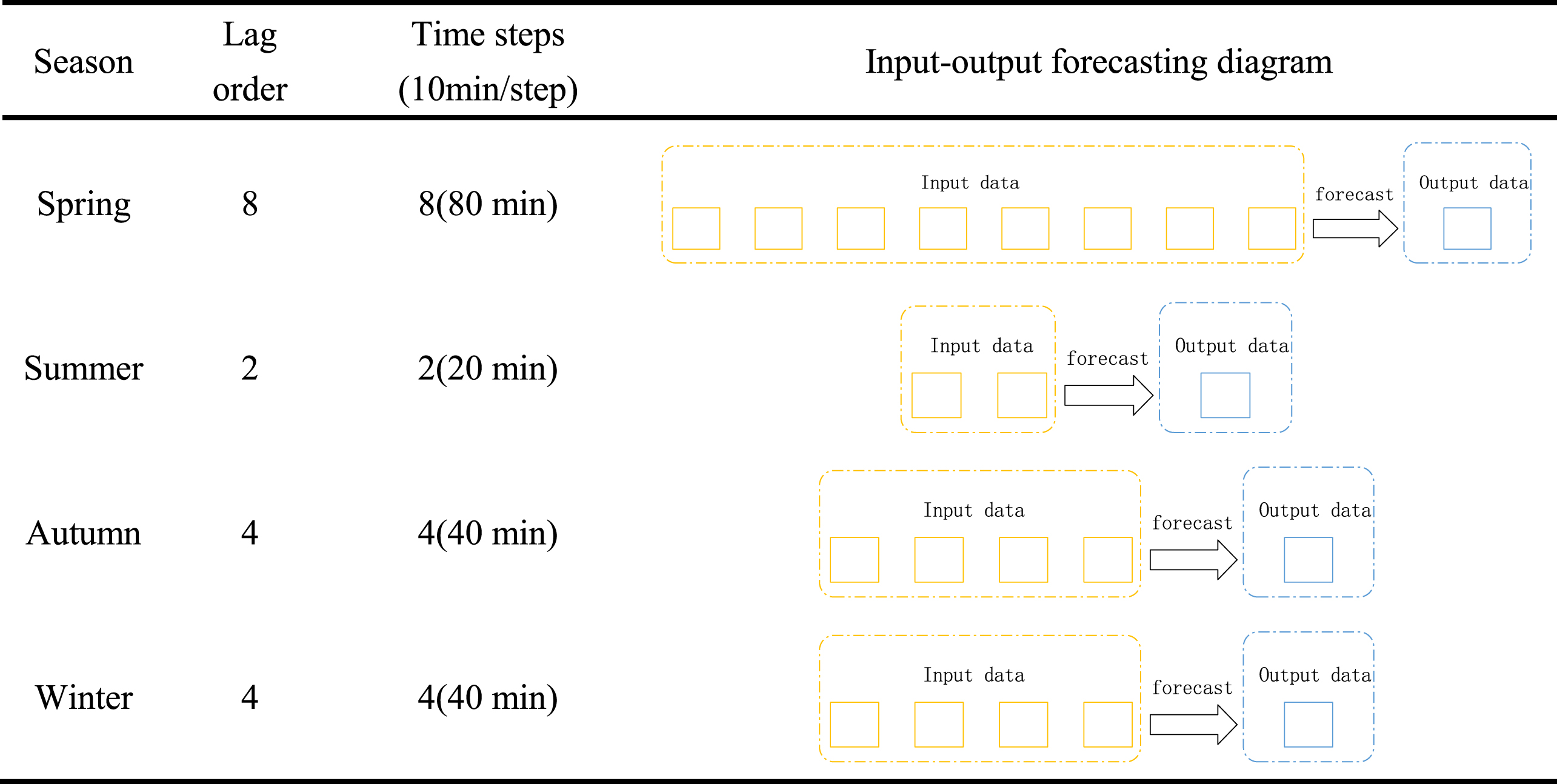
The first action to be taken to predict the wind speed time series is to calculate the lag order and then determine the time steps. The ADF test is used to find the time steps of the four wind speed series, and the results are presented in Table 4.

Table 4
Time steps and input-output forecasting diagram

3.4 Decomposition of data

The original wind speed series are highly volatile and nonlinear, which is difficult to be used directly for wind speed prediction and the final prediction accuracy is bound to be low. It is a good thing that CEEMDAN is very adept at handling these unfavorable characteristics of wind speed series for prediction and modeling. Taking the spring dataset as an example, by default, this spring series will be decomposed into 7 sub-series and 1 residual using CEEMDAN. In this paper, the residual is regarded as the last IMF sub-series, that is, the number of IMF obtained from the decomposition is 8. It is experimentally known that the decomposition result by default is not necessarily optimal, so it is essential to redefine the number of IMFs after decomposition.

Sample entropy (SE) enables to evaluate the complexity of a series, the smaller its value, the lower the complexity. Hence, SE is utilized to analyze the complexity of each sub-series, and the sub-series with lower complexity can be combined to determine the optimal number of decomposed sub-series.

For a time series X of length N, its SE is calculated as follows [45, 46].

Form a vector sequence of dimension m.

$X (i) = {x (i), x (i + 1), \dots, x (i + m - 1)}$ (23)

Calculate the distance between vectors X (i) and X (j).

$\begin{matrix} d [X (i), X (j)] (i \neq j) \\ = \max_{k = 0, \dots, m - 1} (| x (i + k) - x (j + k) |) \end{matrix}$ (24)

Given a threshold r (r > 0), count the number B_i of d [X (i) , X (j)] < r and calculate its ratio to the total number of d [X (i) , X (j)].

$B_{i}^{m} (r) = \frac{B_{i}}{N - m}$ (25)

Calculate the average value of $B_{i}^{m} (r)$ .

$B^{m} (r) = \frac{1}{N - m + 1} \sum_{i = 1}^{N - m + 1} B_{i}^{m} (r)$ (26)

Then add the dimension m by 1 and repeat the above steps (1) (4) to obtain B^m+1 (r).

Lastly, the SE of the time series X is:

$SampEn (m, r, N) = - \ln \frac{B^{m + 1} (r)}{B^{m} (r)}$ (27)

Table 5 demonstrates the calculated SE values of 8 sub-series, from which we find that the SE values of IMF6 IMF8 are less than 0.1, closer to 0. This indicates that the three sub-series have a low complexity, so them are combined to get a new sub-series, which means that the wind speed series will be finally decomposed into 6 sub-series. Figure 7 illustrates the final decomposition result.

Table 5

The SE values of 8 sub-series after CEEMDAN

Sub -series	IMF1	IMF2	IMF3	IMF4	IMF5	IMF6	IMF7	IMF8(Residue)
SE	0.6022	0.4292	0.3810	0.3242	0.1577	0.0587	0.0091	0.0012

Fig. 7

The final decomposition result after CEEMDAN and SE analysis.

It can be seen from Fig. 7 that the original wind speed series is decomposed by CEEMDAN into 6 sub-series arranged from high frequency to low frequency, among which the IMF1 sub-series with the highest frequency has the largest SE value, indicating that it has the highest complexity and is the main source of prediction error. Hence, VMD is employed for the secondary decomposition of IMF1. The four secondary sub-series decomposed into are illustrated in Fig. 8. Obviously, these four secondary sub-series are more regular and predictable.

Fig. 8

The secondary sub-series diagrams after VMD.

3.5 Parameters optimization

After secondary decomposition, the spring wind speed series will be converted into multiple sub-series, which have different characteristics. Accordingly, the parameters of the corresponding DBN for modeling and predicting them separately must be unequal. Besides, the parameters of the initial DBN do not necessarily lead to satisfactory prediction results. Therefore, the parameters optimization of DBN for each sub-series is performed using CSA to search the respective optimal parameters. In building the DBN prediction model, the number of RBM, learning rate and batch size in DBN have a large impact on the prediction accuracy, thus, they naturally become the objects of optimization, according to which the fitness function of CSA is set as shown in Equation (28).

${\begin{matrix} minf (number_of_RBM, learning_rate, batch_size) = \frac{1}{T} \sum_{t = 1}^{T} {(y_{t} - {\bar{y}}_{t})}^{2} \\ number_of_RBM \in [number_of_R {BM}_{\min}, number_of_R {BM}_{\max}] \\ s . t . learning_rate \in [learning_r {ate}_{\min}, learning_r {ate}_{\max}] \\ batch_size \in [batch_s {ize}_{\min}, batch_s {ize}_{\max}] \end{matrix}$ (28)

Furthermore, the parameters are optimized based on the algorithmic flow of CSA in Fig. 5, and the obtained results are given in Table 6.

Table 6

Parameters optimization results of DBN

Sub -series	Number_of_RBM	Learning_rate	Batch_size
u1	270	0.000414	2
u2	254	0.000360	2
u3	264	0.000418	2
u4	252	0.000540	2
IMF2	235	0.000511	2
IMF3	245	0.000303	3
IMF4	246	0.000300	2
IMF5	244	0.000571	3
IMF6(Residue)	247	0.000542	2

4 Experiments and discussions

In this section, for evaluating the performance of the developed parsimonious ensemble model, two different comparison experiments are set up using four season datasets. The improvements of the developed parsimonious ensemble model relative to other models, forecasting error variances of all models and statistical tests are also discussed.

4.1 Ablation experiment

The ablation experiment is specifically represented by comparing CEEMDAN-VMD-DBN-CSA with CEEMDAN-VMD-DBN, CEEMDAN-DBN and DBN, respectively. This experiment embodies the construction process of the proposed model and aims to verify the effectiveness of each component of the model. The evaluation index results of each model over four seasons are shown in Table 7, and the corresponding histograms are presented in Fig. 9. Figure 10 illustrates the prediction series for each model over four seasons. The specific analysis are as follows.

Fig. 9

Predictive performance for each model in the ablation experiment.

Fig. 10

Prediction series for each model in the ablation experiment.

Table 7

Evaluation index results of each model in the ablation experiment

Season	Model	RMSE	MAE	MAPE	R ²
Spring (April)	DBN	0.5912	0.4312	11.7830%	0.9559
	CEEMDAN-DBN	0.4050	0.2885	7.8616%	0.9793
	CEEMDAN-VMD-DBN	0.3322	0.2369	6.3409%	0.9861
	CEEMDAN-VMD-DBN-CSA	0.2898	0.2135	5.8110%	0.9894
Summer (July)	DBN	0.5480	0.4210	8.1642%	0.9568
	CEEMDAN-DBN	0.4305	0.3433	6.4856%	0.9734
	CEEMDAN-VMD-DBN	0.3755	0.3004	5.8901%	0.9797
	CEEMDAN-VMD-DBN-CSA	0.3486	0.2821	5.6142%	0.9825
Autumn (October)	DBN	0.5030	0.3792	6.8396%	0.9506
	CEEMDAN-DBN	0.4105	0.3196	6.0473%	0.9671
	CEEMDAN-VMD-DBN	0.3040	0.2457	4.6027%	0.9819
	CEEMDAN-VMD-DBN-CSA	0.2815	0.2284	4.2335%	0.9845
Winter (January)	DBN	0.6871	0.5212	8.8757%	0.9332
	CEEMDAN-DBN	0.4434	0.3438	5.7156%	0.9722
	CEEMDAN-VMD-DBN	0.3649	0.2820	4.6301%	0.9812
	CEEMDAN-VMD-DBN-CSA	0.3371	0.2633	4.3271%	0.9839

From Table 7 and Fig. 9, we can learn that CEEMDAN-VMD-DBN-CSA achieves the smallest RMSE, MAE, and MAPE among all models regardless of the seasonal datasets of spring, summer, autumn, and winter, and the smaller the values of these three evaluation indexes, the better the corresponding prediction performance, which indicates that the proposed CEEMDAN-VMD-DBN-CSA model performs best.

Based on the data in Table 7, comparing DBN with CEEMDAN-DBN, CEEMDAN-DBN with CEEMDAN-VMD-DBN, and CEEMDAN-VMD-DBN with CEEMDAN-VMD-DBN-CSA, we can find that from DBN to CEEMDAN-VMD-DBN-CSA, the prediction effect continuously becomes better, which means that the prediction performance also keeps improving. Therefore, the effectiveness of CEEMDAN, VMD and CSA can be demonstrated.

From DBN to CEEMDAN-VMD-DBN-CSA, the values of RMSE, MAE, and MAPE decrease significantly. In the case of MAPE, the reduction is 5.9720% in spring, 2.5500% in summer, 2.6061% in autumn and 4.5486% in winter. This indicates that the proposed model remarkably improves the prediction accuracy and highlights its excellent prediction performance.

CONCLUSION: Based on the corresponding graphical presentation and the above analysis, it can be judged that the designed CEEMDAN-VMD-DBN-CSA model outperforms the other three models and therefore, it is valuable.

4.2 Popular model comparison experiment

To further test the usability of the designed model, this experiment compares the new model with two types of popular prediction models. In the first type, some basic models including ELM, RBFNN, LSTM, GRU, CNN and SVR are compared with the designed model to verify its superiority. For the second type, three comprehensive models, including EEMD-ELM-GWO, VMD-LSTM-PSO and EMD-GRU-DE, are utilized to compare with the designed model for a thorough evaluation. In this experiment, the results of the four evaluation indexes for each model over four seasons are given in Table 8, and the corresponding histograms are shown in Fig. 11, as well as the prediction series for each model over four seasons are presented in Fig. 12. The relevant analysis are described below.

Table 8
Evaluation index results for each model over four seasons

Season Model RMSE MAE MAPE R ²

Spring (April) ELM 0.6247 0.4410 11.7300% 0.9507

RBFNN 0.6223 0.4494 11.2444% 0.9511

LSTM 0.7155 0.5443 15.3830% 0.9354

GRU 0.6011 0.4459 12.3686% 0.9544

CNN 0.6171 0.4589 12.9199% 0.9519

SVR 0.7406 0.5752 16.3370% 0.9308

EEMD-ELM-GWO 0.4615 0.3776 10.4793% 0.9731

VMD-LSTM-PSO 0.3377 0.2471 7.1813% 0.9856

EMD-GRU-DE 0.3606 0.2744 7.4670% 0.9836

CEEMDAN-VMD-DBN-CSA 0.2898 0.2135 5.8110% 0.9894

Summer (July) ELM 0.5849 0.4322 7.9630% 0.9508

RBFNN 0.6840 0.5344 12.4628% 0.9328

LSTM 0.6536 0.5297 11.7970% 0.9386

GRU 0.5747 0.4513 9.6526% 0.9525

CNN 0.5900 0.4566 8.9947% 0.9500

SVR 0.6361 0.4932 11.4751% 0.9418

EEMD-ELM-GWO 0.4395 0.3362 6.1679% 0.9722

VMD-LSTM-PSO 0.4256 0.3375 7.0022% 0.9740

EMD-GRU-DE 0.3989 0.3129 6.1162% 0.9771

CEEMDAN-VMD-DBN-CSA 0.3486 0.2821 5.6142% 0.9825

Autumn (October) ELM 0.5174 0.3852 7.4930% 0.9477

RBFNN 0.5148 0.4113 8.6314% 0.9482

LSTM 0.5953 0.4583 8.5039% 0.9308

GRU 0.5150 0.3934 7.2439% 0.9482

CNN 0.5171 0.3910 6.9945% 0.9478

SVR 0.5245 0.4089 8.8098% 0.9463

EEMD-ELM-GWO 0.3829 0.2442 4.3542% 0.9714

VMD-LSTM-PSO 0.4158 0.3384 6.2052% 0.9662

EMD-GRU-DE 0.3984 0.2978 5.2814% 0.9690

CEEMDAN-VMD-DBN-CSA 0.2815 0.2284 4.2335% 0.9845

Winter (January) ELM 0.7298 0.5469 8.7847% 0.9246

RBFNN 0.7894 0.6044 9.8174% 0.9118

LSTM 0.7780 0.5844 10.1055% 0.9144

GRU 0.7059 0.5338 9.1312% 0.9295

CNN 0.7007 0.5360 9.1623% 0.9305

SVR 0.8855 0.6510 10.9058% 0.8890

EEMD-ELM-GWO 0.5114 0.3853 6.2505% 0.9630

VMD-LSTM-PSO 0.3934 0.3155 5.3190% 0.9781

EMD-GRU-DE 0.4629 0.3622 5.8874% 0.9697

CEEMDAN-VMD-DBN-CSA 0.3371 0.2633 4.3271% 0.9839

Season	Model	RMSE	MAE	MAPE	R ²
Spring (April)	ELM	0.6247	0.4410	11.7300%	0.9507
	RBFNN	0.6223	0.4494	11.2444%	0.9511
	LSTM	0.7155	0.5443	15.3830%	0.9354
	GRU	0.6011	0.4459	12.3686%	0.9544
	CNN	0.6171	0.4589	12.9199%	0.9519
	SVR	0.7406	0.5752	16.3370%	0.9308
	EEMD-ELM-GWO	0.4615	0.3776	10.4793%	0.9731
	VMD-LSTM-PSO	0.3377	0.2471	7.1813%	0.9856
	EMD-GRU-DE	0.3606	0.2744	7.4670%	0.9836
	CEEMDAN-VMD-DBN-CSA	0.2898	0.2135	5.8110%	0.9894
Summer (July)	ELM	0.5849	0.4322	7.9630%	0.9508
	RBFNN	0.6840	0.5344	12.4628%	0.9328
	LSTM	0.6536	0.5297	11.7970%	0.9386
	GRU	0.5747	0.4513	9.6526%	0.9525
	CNN	0.5900	0.4566	8.9947%	0.9500
	SVR	0.6361	0.4932	11.4751%	0.9418
	EEMD-ELM-GWO	0.4395	0.3362	6.1679%	0.9722
	VMD-LSTM-PSO	0.4256	0.3375	7.0022%	0.9740
	EMD-GRU-DE	0.3989	0.3129	6.1162%	0.9771
	CEEMDAN-VMD-DBN-CSA	0.3486	0.2821	5.6142%	0.9825
Autumn (October)	ELM	0.5174	0.3852	7.4930%	0.9477
	RBFNN	0.5148	0.4113	8.6314%	0.9482
	LSTM	0.5953	0.4583	8.5039%	0.9308
	GRU	0.5150	0.3934	7.2439%	0.9482
	CNN	0.5171	0.3910	6.9945%	0.9478
	SVR	0.5245	0.4089	8.8098%	0.9463
	EEMD-ELM-GWO	0.3829	0.2442	4.3542%	0.9714
	VMD-LSTM-PSO	0.4158	0.3384	6.2052%	0.9662
	EMD-GRU-DE	0.3984	0.2978	5.2814%	0.9690
	CEEMDAN-VMD-DBN-CSA	0.2815	0.2284	4.2335%	0.9845
Winter (January)	ELM	0.7298	0.5469	8.7847%	0.9246
	RBFNN	0.7894	0.6044	9.8174%	0.9118
	LSTM	0.7780	0.5844	10.1055%	0.9144
	GRU	0.7059	0.5338	9.1312%	0.9295
	CNN	0.7007	0.5360	9.1623%	0.9305
	SVR	0.8855	0.6510	10.9058%	0.8890
	EEMD-ELM-GWO	0.5114	0.3853	6.2505%	0.9630
	VMD-LSTM-PSO	0.3934	0.3155	5.3190%	0.9781
	EMD-GRU-DE	0.4629	0.3622	5.8874%	0.9697
	CEEMDAN-VMD-DBN-CSA	0.3371	0.2633	4.3271%	0.9839

Fig. 11

Predictive performance for each model over four seasons.

Fig. 12

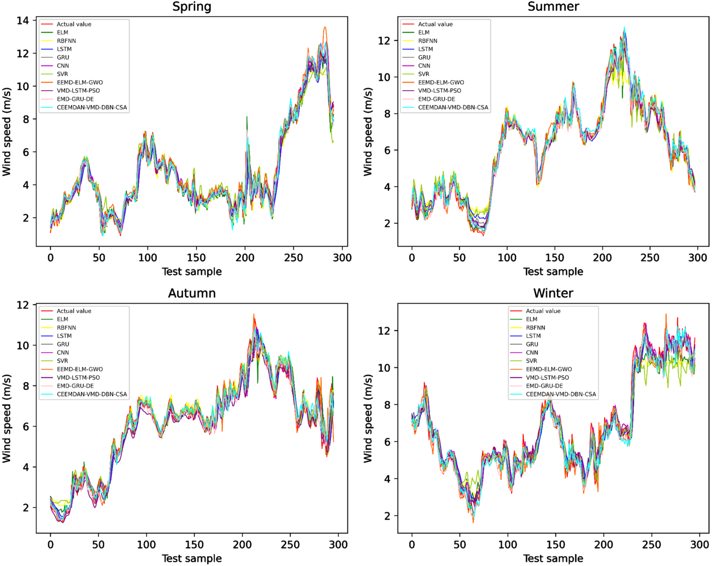
Prediction series for each model over four seasons.

Based on the numerical values exhibited in Table 8, the average R² of each model is calculated, the values of ELM, RBFNN, LSTM, GRU, CNN, SVR EEMD-ELM-GWO, VMD-LSTM-PSO, EMD-GRU-DE, CEEMDAN-VMD-DBN-CSA are 0.9435, 0.9360, 0.9298, 0.9462, 0.9451, 0.9270, 0.9699, 0.9760, 0.9749, 0.9851, respectively. Obviously, the proposed CEEMDAN-VMD-DBN-CSA model obtains the largest average R², which is sufficiently larger than the smallest SVR by 0.0581. Therefore, the proposed model is superior and has a significant advantage over the above basic and comprehensive models.

According to the intuitive values in Table 8 and the height of the columns in Fig. 11, the designed model achieves minimum MAPE in all seasons. It has an average MAPE of 4.9965%, while the other three comprehensive models, EEMD-ELM-GWO, VMD-LSTM-PSO and EMD-GRU-DE, have an average MAPE of 6.8130%, 6.4269% and 6.1880%, respectively, which shows that the average MAPE of the designed models is all more than 1% smaller than theirs. Besides, the designed model makes an outstanding contribution in terms of reducing RSME and MAE, which is shown to have the smallest RSME and MAE among all models. Therefore, the prediction accuracy of the designed model is excellent.

CONCLUSION: In light of the above comprehensive analysis, the designed model has the best RMSE, MAE, MAPE and R² values, which means it possesses the highest prediction accuracy. Thus, it is accurate and valid.

4.3 Improvement percentage

In this subsection, the improvement percentages of the three evaluation indexes (RMSE, MAE and MAPE) in two categories of situation are discussed, the corresponding calculation formula are as follows.

$P_{RMSE} = \frac{{RMSE}_{1} - {RMSE}_{2}}{{RMSE}_{1}} \times 100 %$ (29)

$P_{MAE} = \frac{{MAE}_{1} - {MAE}_{2}}{{MAE}_{1}} \times 100 %$ (30)

$P_{MAPE} = \frac{{MAPE}_{1} - {MAPE}_{2}}{{MAPE}_{1}} \times 100 %$ (31)

The first category of situation refers to the intercomparison of DBN, CEEMDAN-DBN, CEEMDAN-VMD-DBN and CEEMDAN-VMD-DBN-CSA to verify the contribution of each component to the designed model. The corresponding improvement percentages are listed in Table 9, from which it is clear that the improvement percentages obtained from each group comparison are considerable, moreover, the last group of CEEMDAN-VMD-DBN-CSA compared with DBN obtains amazing improvement percentage values. These comparative results demonstrate the great contribution of CEMMDAN, VMD and CSA to the model.

Table 9

Improvement percentages for each component over four seasons

Improvement percentage (%)	Spring	Summer	Autumn	Winter
CEEMDAN-DBN vs. DBN
RMSE	31.50	21.44	18.39	35.47
MAE	33.09	18.46	15.72	34.04
MAPE	33.28	20.56	11.58	35.60
CEEMDAN-VMD-DBN vs. CEEMDAN-DBN
RMSE	17.98	12.78	25.94	17.70
MAE	17.89	12.50	23.12	17.98
MAPE	19.34	9.18	23.89	18.99
CEEMDAN-VMD-DBN-CSA vs. CEEMDAN-VMD-DBN
RMSE	12.76	7.16	7.40	7.62
MAE	9.88	6.09	7.04	6.63
MAPE	8.36	4.68	8.02	6.54
CEEMDAN-VMD-DBN-CSA vs. DBN
RMSE	50.98	36.39	44.04	50.94
MAE	50.49	32.99	39.77	49.48
MAPE	50.68	31.23	38.10	51.25

Then, the second category of situation refers to comparing the designed novel model with various popular models in realizing a comprehensive analysis regarding the extent of improvement in prediction performance. The specific results are given in Table 10, from which it is known that the designed model has a remarkable improvement whether it is a classical basic model or a comprehensive hybrid model. As a result, the designed CEEMDAN-VMD-DBN-CSA model achieves a desirable improvement in prediction performance.

Table 10

Improvement percentages of the designed model relative to various models

Improvement percentage (%)	Spring	Summer	Autumn	Winter
RMSE
ELM	53.61	40.40	45.59	53.81
RBFNN	53.43	49.04	45.32	57.30
LSTM	59.50	46.66	52.71	56.67
GRU	51.79	39.34	45.34	52.25
CNN	53.04	40.92	45.56	51.89
SVR	60.87	45.20	46.33	61.93
EEMD-ELM-GWO	37.20	20.68	26.48	34.08
VMD-LSTM-PSO	14.18	18.09	32.30	14.31
EMD-GRU-DE	19.63	12.61	29.34	27.18
MAE
ELM	51.59	34.73	40.71	51.86
RBFNN	52.49	47.21	44.47	56.44
LSTM	60.78	46.74	50.16	54.95
GRU	52.12	37.49	41.94	50.67
CNN	53.48	38.22	41.59	50.88
SVR	62.88	42.80	44.14	59.55
EEMD-ELM-GWO	43.46	16.09	6.47	31.66
VMD-LSTM-PSO	13.60	16.41	32.51	16.55
EMD-GRU-DE	22.19	9.84	23.30	27.31
MAPE
ELM	50.46	29.50	43.50	50.74
RBFNN	48.32	54.95	50.95	55.92
LSTM	62.22	52.41	50.22	57.18
GRU	53.02	41.84	41.56	52.61
CNN	55.02	37.58	39.47	52.77
SVR	64.43	51.07	51.95	60.32
EEMD-ELM-GWO	44.55	8.98	2.77	30.77
VMD-LSTM-PSO	19.08	19.82	31.77	18.65
EMD-GRU-DE	22.18	8.21	19.84	26.50

4.4 Forecasting error variance

Stability is an important aspect of model performance, in this subsection, the forecasting error variance (FEVar) is utilized to validate the stability of all models and thus evaluate their performance more clearly. The specific formula is presented below.

$E r r_{t} = y_{t}^{i} - y_{t}$ (32)

$FEVar = \frac{1}{T} \sum_{t = 1}^{T} {({Err}_{t} - \bar{Err})}^{2}$ (33)

in which y_t, , Err_t and $\bar{Err}$ are the actual value, forecasting value, forecasting error and average of forecasting error, respectively.

The smaller the FEVar, the better the stability of the corresponding model. And the FEVar of each model over four seasons are displayed in Table 11, from which it is known that the proposed model achieves the smallest FEVars of 0.0819, 0.1007, 0.0760 and 0.0994 for Spring, Summer, Autumn and Winter, respectively. Thus, the proposed CEEMDAN-VMD-DBN-CSA model has the highest stability in comparison with other models. Additionally, DBN also has a smaller FEVar than ELM, RBFNN, LSTM, GRU, CNN and SVR regardless of which seasonal dataset, which is evidence that DBN outperforms other single models in terms of stability.

Table 11

FEVar of each model over four seasons

FEVar	Spring	Summer	Autumn	Winter
ELM	0.3899	0.3410	0.2674	0.5103
RBFNN	0.3789	0.4651	0.2610	0.6093
LSTM	0.5119	0.4272	0.3480	0.6048
GRU	0.3613	0.3282	0.2610	0.4981
CNN	0.3685	0.3481	0.2566	0.4795
SVR	0.5298	0.4033	0.2742	0.7724
EEMD-SVR-GWO	0.1416	0.1923	0.1466	0.1958
VMD-LSTM-PSO	0.1132	0.1808	0.0816	0.1541
EMD-GRU-DE	0.1287	0.1513	0.1410	0.1442
DBN	0.3493	0.2997	0.2483	0.4707
CEEMDAN-DBN	0.1609	0.1845	0.1483	0.1778
CEEMDAN-VMD-DBN	0.1103	0.1267	0.0875	0.1141
CEEMDAN-VMD-DBN-CSA	0.0819	0.1007	0.0760	0.0994

4.5 Statistical tests

With the aim of fully confirming the outstanding contribution and superiority of the proposed CEEMDAN-VMD-DBN-CSA model, we perform two statistical tests namely Wilcoxon signed-rank test (test ding172) and Friedman test (test ding173) in this research. Among them, test ding172; is a non-parametric statistical test for detecting whether there is a significant difference in the central tendencies of two data series (with the same amount of data), while test ding173 is used to judge the significant difference between three or more related samples [47, 48]. They are both applicable in cases where the data of the related samples do not satisfy a normal distribution.

For test ding172, the original hypothesis H₀ is that there is no significant difference in the predictive effectiveness of the two models, in test ding173 it is the case that there is no significant difference in the predictive effectiveness of all competitive models, i.e., e₁ = e₂ = e₃ = e₄ = e₅ = e₆ = e₇ = e₈ = e₉ = e₁₀. Both tests are conducted at a significance level of α=0.05 [49]. When p-value >0.05, H₀ is accepted, i.e., the forecasting effectiveness of this group of comparative models are the same; when p-value <0.05, H₀ is rejected, indicating that the forecasting effectiveness of this group of comparative models are different.

Table 12 shows the results of the two tests for four seasons. It is worth noting that the CEEMDAN-VMD-DBN-CSA model is the benchmark and the other nine models in the table are compared with it. In Table 12, it is clear that the p-values based on test ding172 are all less than 0.05 except for the ELM model in winter season, which means that all of them fulfill the requirement and H₀ is rejected. Besides, it is evident that the p-values based on test ding173 are much smaller than 0.05 in all four seasons and H₀ is rejected.

Table 12
Results of the two tests: CEEMDAN-VMD-DBN-CSA model as benchmark

Season Compared model Wilcoxon signed-rank test p-value Friedman test

Spring ELM 3.48E-03 p = 0.0000(Reject H₀)

RBFNN 2.03E-05

LSTM 4.01E-02

GRU 1.31E-02

CNN 1.31E-03

SVR 2.52E-04

EEMD-ELM-GWO 4.06E-25

VMD-LSTM-PSO 4.31E-02

EMD-GRU-DE 2.45E-02

Summer ELM 8.13E-11 p = 0.0000 (Reject H₀)

RBFNN 4.43E-03

LSTM 1.99E-06

GRU 7.05E-05

CNN 4.45E-08

SVR 2.05E-04

EEMD-ELM-GWO 3.43E-14

VMD-LSTM-PSO 7.11E-15

EMD-GRU-DE 9.61E-41

Autumn ELM 3.93E-04 p = 0.0000 (Reject H₀)

RBFNN 2.82E-02

LSTM 6.14E-07

GRU 1.43E-07

CNN 6.12E-12

SVR 3.75E-02

EEMD-ELM-GWO 8.91E-07

VMD-LSTM-PSO 6.68E-48

EMD-GRU-DE 6.38E-33

Winter ELM 9.77E-02 p = 0.0000 (Reject H₀)

RBFNN 2.80E-02

LSTM 8.96E-07

GRU 3.50E-07

CNN 3.76E-14

SVR 7.12E-03

EEMD-ELM-GWO 8.84E-14

VMD-LSTM-PSO 2.94E-07

EMD-GRU-DE 3.61E-19

Season	Compared model	Wilcoxon signed-rank test p-value	Friedman test
Spring	ELM	3.48E-03	p = 0.0000(Reject H₀)
	RBFNN	2.03E-05
	LSTM	4.01E-02
GRU	1.31E-02
	CNN	1.31E-03
	SVR	2.52E-04
	EEMD-ELM-GWO	4.06E-25
	VMD-LSTM-PSO	4.31E-02
	EMD-GRU-DE	2.45E-02
Summer	ELM	8.13E-11	p = 0.0000 (Reject H₀)
	RBFNN	4.43E-03
	LSTM	1.99E-06
	GRU	7.05E-05
	CNN	4.45E-08
	SVR	2.05E-04
	EEMD-ELM-GWO	3.43E-14
	VMD-LSTM-PSO	7.11E-15
	EMD-GRU-DE	9.61E-41
Autumn	ELM	3.93E-04	p = 0.0000 (Reject H₀)
	RBFNN	2.82E-02
	LSTM	6.14E-07
	GRU	1.43E-07
	CNN	6.12E-12
	SVR	3.75E-02
	EEMD-ELM-GWO	8.91E-07
	VMD-LSTM-PSO	6.68E-48
	EMD-GRU-DE	6.38E-33
Winter	ELM	9.77E-02	p = 0.0000 (Reject H₀)
	RBFNN	2.80E-02
	LSTM	8.96E-07
	GRU	3.50E-07
	CNN	3.76E-14
	SVR	7.12E-03
	EEMD-ELM-GWO	8.84E-14
	VMD-LSTM-PSO	2.94E-07
	EMD-GRU-DE	3.61E-19

Taking the results of the two statistical tests together, it can be concluded that the forecasting accuracy of the proposed CEEMDAN-VMD-DBN-CSA model is significantly different from that of the other nine comparative models. Moreover, combining the results of the four evaluation indexes in Table 8 and the corresponding analysis, the forecasting accuracy of the proposed model is remarkably superior to other competing models in all four seasons.

5 Conclusion

In this research, a parsimonious ensemble forecasting model consisting of CEEMDAN, VMD, CSA, and individual DBN is designed, which not only eliminates the influence of multiple uncertainties in wind speed, but also only uses DBN as a predictor to achieve parsimonious ensemble and efficient forecasting. The proposed CEEMDAN-VMD-DBN-CSA model is analyzed through specific experimental data and some modeling details. Two experiments are used to evaluate the validity and applicability of the designed model. Three statistical error indexes RMSE, MAE, MAPE and their improvement percentages, as well as R² are used as evaluation methodologies to analyze the prediction performance of different models. In addition, the FEVar is utilized to measure the stability of the designed model and two statistical tests are conducted to demonstrate the superiority of the model.

According to the comparative results of the first experiment, it is clear that: (1) The CEEMDAN-DBN model incorporating the single-level decomposition technique outperforms the basic DBN model, which reveals the contribution of CEEMDAN to improving prediction accuracy; (2) The CEEMDAN-VMD-DBN model with the two-level decomposition technique achieves more satisfactory prediction results than the CEEMDAN-DBN model, it can be judged that the CEEMDAN-VMD decomposition technique is an excellent method; (3) CEEMDAN-VMD-DBN-CSA is superior to CEEMDAN-VMD-DBN, indicating that CSA contributes significantly to performance optimization. As for the second experiment, by comparing the designed model with some basic single models and comprehensive prediction models, it is proved that the designed model has excellent prediction performance. In a word, two experimental results both show that the designed model outperforms various comparative models. This is also demonstrated by the fact that the model achieves the minimum RMSE on all four datasets, and they are 0.2898, 0.3486, 0.2815, and 0.3371, respectively.

In general, the designed model can successfully model the volatility and nonlinearity of wind speed. The combination of CEEMDAN and VMD allows for a significant reduction in the difficulty of prediction, and CSA can well optimize the hyper-parameters of DBN and enhance its learning capability. Thus, the designed CEEMDAN-VMD-DBN-CSA model is effective and trustworthy. However, when determining the input-output data structure, this paper only applies the ADF test to calculate the number of input features without further selecting some features with strong correlation from them. Additionally, in predicting future wind speed, this study only makes one-step prediction, and in real life, multi-step prediction will have a wider range of applications. Therefore, our future research will embark on the following two directions. (1) Consider adding feature selection approaches to the prediction system in order to select some features with strong correlation as the optimal input data, so as to further improve the modeling efficiency and prediction accuracy. (2) We plan to do multi-step wind speed prediction to obtain more prediction results with reference value and improve the practicality of the prediction system.

Footnotes

Acknowledgments

The research was supported by the National Natural Science Foundation of China (Grant No.71971105).

References

Liu

, Lei

, Xu

and Yuan

, China’s energy revolution strategy into, Resources, Conservation and Recycling 128 (2018), 78–89. https://doi.org/10.1016/j.resconrec.2017.09.028

Wang

J.-Z.

, Wang

and Jiang

, The study and application of a novel hybrid forecasting model - A case study of wind speed forecasting in China, Applied Energy 143 (2015), 472–488. https://doi.org/10.1016/j.apEnergy2015.01.038.

Torres

J.L.

, García

and De

, Blas and A. De Francisco, Forecast of hourly average wind speed with ARMA models in Navarre (Spain), Solar Energy 79 (2005), 65–77. https://doi.org/10.1016/j.solener.2004.09.013

Dosdoğru

A.T.

, and A. Boru İpek, Hybrid boosting algorithms and artificial neural network for wind speed prediction, International Journal of Hydrogen Energy 47 (2022), 1449–1460. https://doi.org/10.1016/j.ijhydene.2021

Cinar

A.C.

and Natarajan

, An artificial neural network optimized by grey wolf optimizer for prediction of hourly wind speed in Tamil Nadu, India, Intelligent Systems with Applications 16 (2022), 200138. https://doi.org/10.1016/j.iswa.2022.200138

Shboul

, Al-Arfi

, Michailos

, Ingham

, Ma

and Hughes

K.J.

, et al., A new ANN model for hourly solar radiation and wind speed prediction: A case study over the north & south of the Arabian Peninsula, Sustainable Energy Technologies and Assessments 46 (2021), 101248. https://doi.org/10.1016/j.seta.2021.101248

Tian

, Short-term wind speed prediction based on LMD and improved FA optimized combined kernel function LSSVM, Engineering Applications of Artificial Intelligence 91 (2020), 103573. https://doi.org/10.1016/j.engappai.2020.103573

Liu

, Cao

, Zhang

, Wang

, Huang

and Luo

, Short-term wind speed forecasting based on the Jaya-SVM model, &} }, Energy Systems 121 (2020), 106056. https://doi.org/10.1016/j.ijepes.2020.106056

Zheng

, Ge

, Muhsen

, Wang

, Elkamchouchi

D.H.

, Ali

et al. New ridge regression, artificial neural networks and support vector machine for wind speed prediction, Advances in Engineering Software 179 (2023), 103426. https://doi.org/10.1016/j.advengsoft.2023.103426

10.

Malik

and Yadav

A.K.

, A novel hybrid approach based on relief algorithm and fuzzy reinforcement learning approach for predicting wind speed, Sustainable Energy Technologies and Assessments 43 (2021), 100920. https://doi.org/10.1016/j.seta.2020.100920

11.

Khasanzoda

, Zicmane

, Beryozkina

, Safaraliev

, Sultonov

and Kirgizov

, Regression model for predicting the speed of wind flows for energy needs based on fuzzy logic, Renewable Energy 191 (2022), 723–731. https://doi.org/10.1016/j.renene.2022.04.017

12.

Liu

, Hara

and Kita

, Hybrid forecasting system based on data area division and deep learning neural network for short-term wind speed forecasting, Energy Conversion and Management 238 (2021), 114136. https://doi.org/10.1016/j.enconman.2021.114136

13.

Wang

, Lv

, Li

and Zeng

, Multivariate selection-combination short-term wind speed forecasting system based on convolution-recurrent network and multi-objective chameleon swarm algorithm, Expert Systems with Applications 214 (2023), 119129. https://doi.org/10.1016/j.eswa.2022.119129

14.

Wang

, An

, Li

and Lu

, A novel combined forecasting model based on neural networks, deep learning approaches, and multi-objective optimization for short-term wind speed forecasting, Energy 251 (2022), 123960. https://doi.org/10.1016/j.Energy2022.123960

15.

Hao

, Yang

and Yin

, Novel wind speed forecasting model based on a deep learning combined strategy in urban energy systems, Expert Systems with Applications 219 (2023), 119636. https://doi.org/10.1016/j.eswa.2023.119636

16.

Wang

, Li

, Zhang

and Wang

, A deep-learning wind speed interval forecasting architecture based on modified scaling approach with feature ranking and two-output gated recurrent unit, Expert Systems with Applications 211 (2023), 118419. https://doi.org/10.1016/j.eswa.2022.118419

17.

Dong

, Ma

and Fu

, Electrical load forecasting: A deep learning approach based on K-nearest neighbors, Applied Soft Computing 99 (2021), 106900. https://doi.org/10.1016/j.asoc.2020.106900

18.

, Hu

and Fan

, Probabilistic electrical load forecasting for buildings using Bayesian deep neural networks, Journal of Building Engineering 46 (2022), 103853. https://doi.org/10.1016/j.jobe.2021.103853

19.

Zhang

and Ci

, Deep belief network for gold price forecasting, Resources Policy 69 (2020), 101806. https://doi.org/10.1016/j.resourpol.2020.101806

20.

Kamara

A.F.

, Chen

and Pan

, An ensemble of a boosted hybrid of deep learning models and technical analysis for forecasting stock prices, Information Sciences 594 (2022), 1–19. https://doi.org/10.1016/j.ins.2022.02.015

21.

, Wang

, Guo

and Yang

, Research and application of a novel hybrid forecasting system based on multi-objective optimization for wind speed forecasting, Energy Conversion and Management 150 (2017), 90–107. https://doi.org/10.1016/j.enconman.2017.07.065

22.

Zhang

, Zhou

, Li

, Fu

and Peng

, A compound structure of ELM based on feature selection and parameter optimization using hybrid backtracking search algorithm for wind speed forecasting, Energy Conversion and Management 143 (2017), 360–376. https://doi.org/10.1016/j.enconman.2017.04.007

23.

Jaseena

K.U.

and Kovoor

B.C.

, Decomposition-based hybrid wind speed forecasting model using deep bidirectional LSTM networks, Energy Conversion and Management 234 (2021), 113944. https://doi.org/10.1016/j.enconman.2021.113944

24.

Liu

, Duan

, Han

F.-Z.

and Li

Y.-F.

, Big multi-step wind speed forecasting model based on secondary decomposition, ensemble method and error correction algorithm, Energy Conversion and Management 156 (2018), 525–541. https://doi.org/10.1016/j.enconman.2017.11.049

25.

Zhang

, Chen

, Xiao

, Zhang

and Feng

, Hybrid wind speed forecasting model based on multivariate data secondary decomposition approach and deep learning algorithm with attention mechanism, Renewable Energy 174 (2021), 688–704. https://doi.org/10.1016/j.renene.2021.04.091

26.

Zhang

, Qu

, Zhang

, Mao

, Ma

and Fan

, A combined model based on CEEMDAN and modified flower pollination algorithm for wind speed forecasting, Energy Conversion and Management 136 (2017), 439–451. https://doi.org/10.1016/j.enconman.2017.01.022

27.

Zou

, Fu

, Fang

, Xiong

and Wang

, A hybrid model based on multi-stage principal component extraction, GRU network and KELM for multi-step short-term wind speed forecasting, IEEE Access 8 (2020), 222931–222943. https://doi.org/10.1109/ACCESS.2020.3043812

28.

, Xia

, Peng

and Guo

, Detection algorithm for magnetic dipole target based on CEEMDAN and pattern recognition, Procedia Computer Science 183 (2021), 669–676. https://doi.org/10.1016/j.procs.2021.02.113

29.

Jun

, Yuyan

, Lingyu

and Peng

, A new weighted CEEMDAN-based prediction model: An experimental investigation of decomposition and non-decomposition approaches, Knowledge-Based Systems 160 (2018), 188–199. https://doi.org/10.1016/j.knosys.2018.06.033

30.

Shang

, Chen

, Guo

and Yang

, Decomposition-based wind speed forecasting model using causal convolutional network and attention mechanism, Expert Systems with Applications 223 (2023), 119878. https://doi.org/10.1016/j.eswa.2023.119878

31.

Liang

, Zhao

and Shi

, A novel combined model based on VMD and IMODA for wind speed forecasting, Fuzzy Systems 42 (2022), 2845–2861. https://doi.org/10.3233/JIFS-201191

32.

Shi

, Qin

, Tao

and Liu

, A VMD-EWT-LSTM-based multi-step prediction approach for shield tunneling machine cutterhead torque, Knowledge-Based Systems 228 (2021), 107213. https://doi.org/10.1016/j.knosys.2021.107213

33.

Sun

, Zhao

and Zhao

, Hybrid model based on VMD decomposition, clustering analysis, long short memory network, ensemble learning and error complementation for short-term wind speed forecasting assisted by Flink platform, Energy 261 (2022), 125248. https://doi.org/10.1016/j.Energy2022.125248

34.

Chan

R.H.

, Tao

and Yuan

, Constrained total variation deblurring models and fast algorithms based on alternating direction method of multipliers, SIAM Journal on Imaging Sciences 6 (2013), 680–697. https://doi.org/10.1137/110860185

35.

Chen

, Lin

, Zhao

, Wang

and Gu

, Deep learning-based classification of hyperspectral data, IEEE Journal of Selected Topics in Applied Earth Observations and Remote Sensing 7 (2014), 2094–2107. https://doi.org/10.1109/JSTARS.2014.2329330

36.

Hinton

G.E.

, Osindero

and Teh

Y.-W.

, A fast learning algorithm for deep belief nets, Neural Computation 18 (2006), 1527–1554. https://doi.org/10.1162/neco.2006.18.7.1527

37.

Saleem

, Khattak

M.I.

, Al-Hasan

M.A.

and Jan

, Learning time-frequency mask for noisy speech enhancement using gaussian-bernoulli pre-trained deep neural networks, Fuzzy Systems 40 (2021), 849–864. https://doi.org/10.3233/JIFS-201014

38.

Zhong

, Qu

, Fang

, Li

and Wang

, The intermittent fault diagnosis of analog circuits based on EEMD-DBN, Neurocomputing 436 (2021), 74–91. https://doi.org/10.1016/j.neucom.2021.01.001

39.

Hinton

G.E.

A practical guide to training restricted Boltz mann machines, in: G. Montavon, G.B. Orr, K.-R. Müller, (Eds.), Neural Networks: Tricks of the Trade: Second Edition, Springer Berlin Heidelberg, Berlin, Heidelberg, 2012. pp. 599–619. https://doi.org/10.1007/978-3-642-35289-8_32

40.

Zhou

, Huang

, Zhang

, Ma

and Feng

, Prediction of jacking force using PSO-BPNN and PSO-SVR algorithm in curved pipe roof, Tunnelling and Underground Space Technology 138 (2023), 105159. https://doi.org/10.1016/j.tust.2023.105159

41.

Hrasko

, Pacheco

A.G.C.

and Krohling

R.A.

, Time series prediction using restricted Boltzmann machines and backpropagation, Procedia Computer Science 55 (2015), 990–999. https://doi.org/10.1016/j.procs.2015.07.104

42.

Aliabadi

M.J.

and Radmehr

, Optimization of hybrid renewable energy system in radial distribution networks considering uncertainty using meta-heuristic crow search algorithm, Applied Soft Computing 107 (2021), 107384. https://doi.org/10.1016/j.asoc.2021.107384

43.

L.-L.

, Liu

Z.-F.

, Tseng

M.-L.

, Jantarakolica

and Lim

M.K.

, Using enhanced crow search algorithm optimization-extreme learning machine model to forecast short-term wind power, Expert Systems with Applications 184 (2021), 115579. https://doi.org/10.1016/j.eswa.2021.115579

44.

Adamu

, Abdullahi

, Junaidu

S.B.

and Hassan

I.H.

, An hybrid particle swarm optimization with crow search algorithm for feature selection, Machine Learning with Applications 6 (2021), 100108. https://doi.org/10.1016/j.mlwa.2021.100108.

45.

Richman

J.S.

and Moorman

J.R.

, Physiological time-series analysis using approximate entropy and sample entropy, American Journal of Physiology-Heart and Circulatory Physiology 278 (2039), H2039–H2049. https://doi.org/10.1152/ajpheart.2000.278.6.H2039

46.

Peng

, Zhang

, Zhou

and Nazir

M.S.

, Negative correlation learning-based RELM ensemble model integrated with OVMD for multi-step ahead wind speed forecasting, Renewable Energy 156 (2020), 804–819. https://doi.org/10.1016/j.renene.2020.03.168

47.

Derrac

, García

, Molina

and Herrera

, A practical tutorial on the use of nonparametric statistical tests as a methodology for comparing evolutionary and swarm intelligence algorithms, Swarm and Evolutionary Computation 1 (2011), 3–18. https://doi.org/10.1016/j.swevo.2011.02.002

48.

M.-W.

, Xu

D.-Y.

, Geng

and Hong

W.-C.

, A hybrid approach for forecasting ship motion using CNN-GRU-AM and GCWOA, Applied Soft Computing 114 (2022), 108084. https://doi.org/10.1016/j.asoc.2021.108084

49.

Zhang

and Hong

W.-C.

, Application of variational mode decomposition and chaotic grey wolf optimizer with support vector regression for forecasting electric loads, {Knowledge-Based Systems 228 (2021), 107297. https://doi.org/10.1016/j.knosys.2021.107297

A parsimonious ensemble with optimal deep learning and secondary decomposition for short-term wind speed forecasting

Abstract

Keywords

Nomenclature

1 Introduction

1.1 Background

1.2 Literature review

1.3 Our work and contributions

2 Methodology and model framework

2.1 CEEMDAN

2.3.1 RBM

3.1 Dataset description

Table 4 Time steps and input-output forecasting diagram

4.1 Ablation experiment

Footnotes

Acknowledgments

References

Table 4
Time steps and input-output forecasting diagram