Research on adaptive circuit structure optimization in electronic design based on Asynchronous Advantage Actor Critic (A3C) algorithm

Abstract

The circuit structure optimizationed with the traditional method is often difficult to meet the complex and changeable design requirements. In this paper the A3C algorithm has been applied to integrate strategy learning and value learning for the circuit structure optimization. This integration can facilitate continuous interaction with the environment, enabling automatic adjustment of circuit structures to meet the complex design requirements. Gain, bandwidth, latency, and power consumption have been set as the optimization objectives, and the actions of the intelligent agent, which include adding, deleting, modifying connection lines, and adjusting component parameters have been introduced in detail. Once the Actor and Critic networks have been established, multiple agents can operate concurrently, translating optimization objectives into reward signals and providing direction and motivation for agent learning. Then with the proposed method, the circuit structure of one switch audio power amplifier has been designed in a simulation environment. The structure optimization results demonstrated that the gain can reach 78.4 dB at convergence of the A3C algorithm, while the bandwidth can reach 156.2 MHz at convergence, and both the circuit delay and power consumption have been reduced significantly. Obviously, the application of the A3C algorithm can effectively optimize the circuit structures through offering more flexible and efficient solutions.

Keywords

Circuit structure adaptive optimization electronic design deep reinforcement learning Asynchronous Advantage Actor-Critic

1 Introduction

As functionality and performance of electronic devices have improved continuously, the electronic design has confronted with increasingly intricate and diverse challenges [1, 2]. Traditional methods of electronic design frequently depend on engineers’ experience and manual adjustments, which have proven insufficient in response to the escalating complexity and variability in design requirements. The Deep Reinforcement Learning method, which adeptly merges the benefits of deep learning and reinforcement learning, can offer a potential solution to these challenges [3, 4]. Through interaction with the surroundings, intelligent agents can extract optimal decision-making strategies from extensive data and experience, thereby facilitating automated optimization processes. Therefore the application of DRL technology facilitates automated optimization of circuit structures, enhancing circuit performance, diminishing power consumption, and reducing area requirements [5, 6].

In this article, an Asynchronous Advantage Actor-Critic (A3C) algorithm has been employed for the circuit structure optimization in order to solve the problems existing in traditional electronic design. The DRL method has been applied to the optimization of circuit structure for the first time, and adaptive adjustment has been realized with A3C algorithm, which can significantly improve the performance and efficiency of the circuit and brings innovative methods to the field of electronic design. Details of abbreviations in this paper are listed in Table 1.

Table 1
Abbreviation details

Abbreviate Full name

A3C Asynchronous Advantage Actor-Critic

DRL Deep Reinforcement Learning

RL Reinforcement Learning

GA Genetic Algorithm

PSO Particle Swarm Optimization

Abbreviate	Full name
A3C	Asynchronous Advantage Actor-Critic
DRL	Deep Reinforcement Learning
RL	Reinforcement Learning
GA	Genetic Algorithm
PSO	Particle Swarm Optimization

2 Methods for optimizing circuit structure

2.1 Related definitions and principles

Optimization of circuit structure is a significant research area of modern electronics [7]. When attempting to meet performance requirements, traditional circuit structures are often constrained by factors such as speed and accuracy [8 –10].

The circuit structure encompasses a diverse array of electronic components and their respective connection methodologies, which are all designed to fulfill specific functions within circuits [11, 12]. An example of this circuit structure has been shown in Fig. 1.

Fig. 1

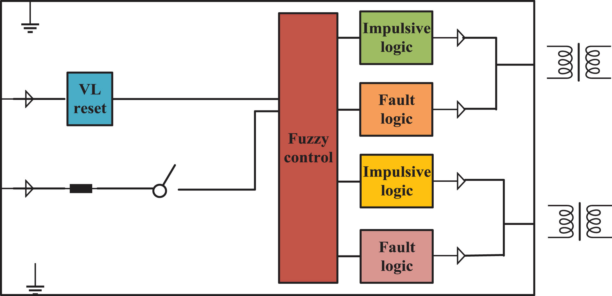
Example of one circuit structure.

The optimization objectives for one circuit structure commonly include gain, bandwidth, latency, and power consumption. However, only one single optimization objective may not satisfy all design requirements. Therefore, multi-objective optimization has been employed to holistically address diverse requirements and attain optimal comprehensive performance. The multi-objective optimization process for the circuit structure has been shown in Fig. 2.

Fig. 2

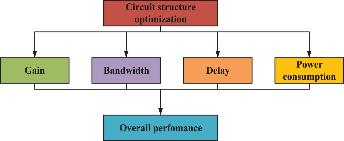
Flow chart of Multi-objective optimization process.

Gain refers to the proportional relationship between a circuit output signal and its input signal. The primary objective of gain optimization is to enhance this relationship, thereby amplifying the input signal more effectively by the circuit. Voltage gain can be characterized as the ratio of the output voltage to the input voltage, the formula of which can be expressed as follows. $A_{v} = \frac{V_{out}}{V_{in}}$ (1)

Bandwidth refers to the frequency range within which a circuit can transmit data. The objective of bandwidth optimization is to enhance this frequency response and augment its signal transmission capability [13, 14]. The formula for calculating the bandwidth is as follows. $BW = f_{high} - f_{low}$ (2)

Where, f_high and f_low are the high and low cutoff frequencies of the amplifier respectively.

Delay refers to the time requisite for signal transmission through a circuit. The primary objective of optimization is to minimize this delay, thereby reducing the circuit’s response time and enhancing its real-time performance [15, 16]. The formula of delay experienced by the transmission line is denoted as follows. $r = \frac{l}{k}$ (3)

Where, k and l represent propagation speed and line length respectively.

Power consumption refers to the energy consumed by a circuit in its working state, and the optimization goal is to minimize power consumption in order to reduce energy consumption and heat generation [17, 18]. The power consumption can be calculated by the current and voltage of the components, and its formula is as follows. $P = IV$ (4)

When optimizing the circuit structure, several constraints must also be met as listed in Table 2.

Table 2

Constraint table

Constraint condition	Description	Requirement
Power supply voltage range	The working power supply voltage range of the circuit	5V–12V
Current limitation	Current limitation of each component in the circuit	100 mA Max
Power consumption limitation	The power consumption of the circuit needs to be within a certain range	1000 mW Max
Bandwidth requirements	The bandwidth requirements that the circuit needs to meet	10 kHz Min
Temperature limit	The operating temperature range of the circuit	–40°C to 85°C
Size limitations	Size limitations of circuit boards	10 cm*10 cm Max
Noise limitation	The noise level of the circuit needs to be within a certain range	50 mVrms Max

In Table 2, the circuit design constraints include power supply voltage range, bandwidth requirement, limitation of current, power consumption, temperature, size and noise. The constraints in circuit design are usually determined by considerations such as functional requirements, reliability, performance requirements, resource limitations, safety and cost, which ensures that the designed circuit structure can meet the requirements and operate normally under various working conditions. The action space of the agents for the circuit structure optimization is shown in Fig. 3.

Fig. 3

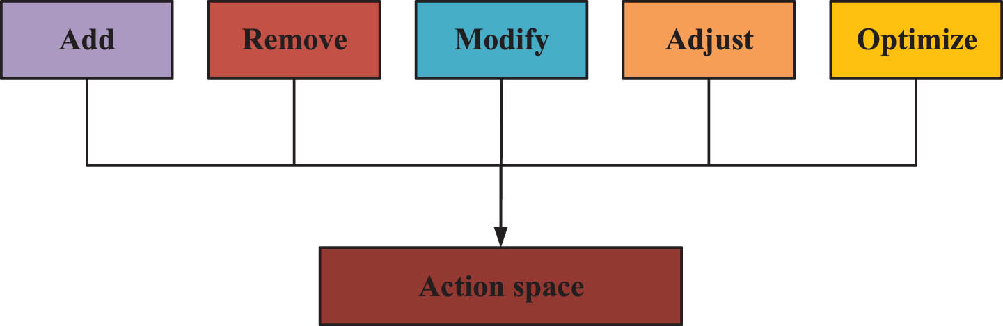
Action space.

By establishing appropriate action spaces, agents can more proficiently navigate the circuit design space, thereby identifying the optimal circuit configuration.

The reward function can be expressed as follows. $Y = w_{1} \cdot s_{1} + w_{2} \cdot s_{2} - w_{3} \cdot s_{3} - w_{4} \cdot s_{4}$ (5)

Where, s₁, s₂, s₃, s₄ represent gain, bandwidth, delay, and power consumption, while w₁, w₂, w₃, w₄ represent the corresponding weights respectively.

The goal of the optimizing can be expressed as follows. $U = (s_{1} + s_{2} - s_{3} - s_{4}) / 4$ (6)

2.2 Introduction of A3C algorithm

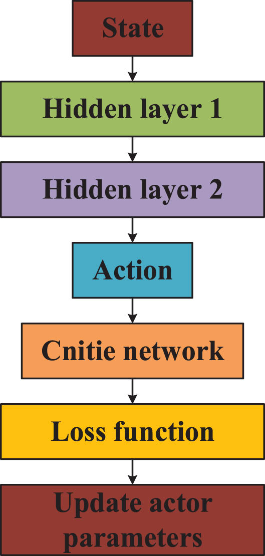
The A3C algorithm is one method of parallelization utilized in training Deep Reinforcement Learning (DRL) models, which integrates the principles of both the Actor-Critic algorithm and multi-threaded parallel computing [19]. This algorithm can gather empirical data through the simultaneous operation of multiple agents, employing a global critical network to assess the quality of these experiences and subsequently guide the agent updates. The architecture of the Actor and Critic networks have been illustrated in Figs. 4 and 5 respectively [20].

Fig. 4

Architecture of the Actor network.

Fig. 5

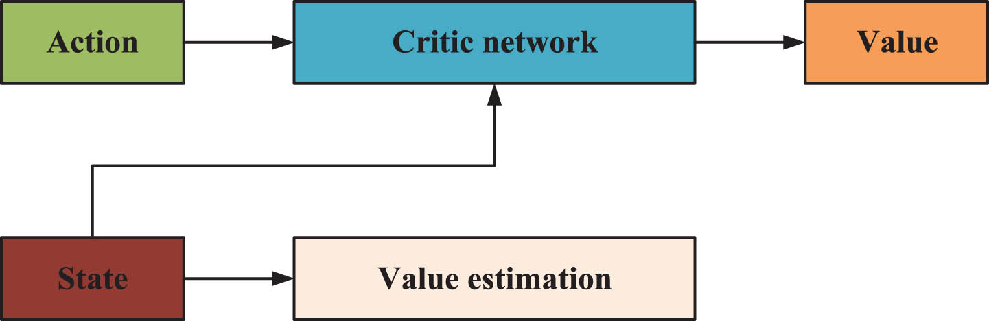
Architecture of the Critic network.

The A3C algorithm is based on the Actor-Critic architecture, which includes two neural networks, which are the Actor network and the Critic network. The former is responsible for selecting actions based on the current state, while the later is responsible for evaluating the value of actions [21, 22].

The structure of the Actor-Critic algorithm is shown in Fig. 6.

Fig. 6

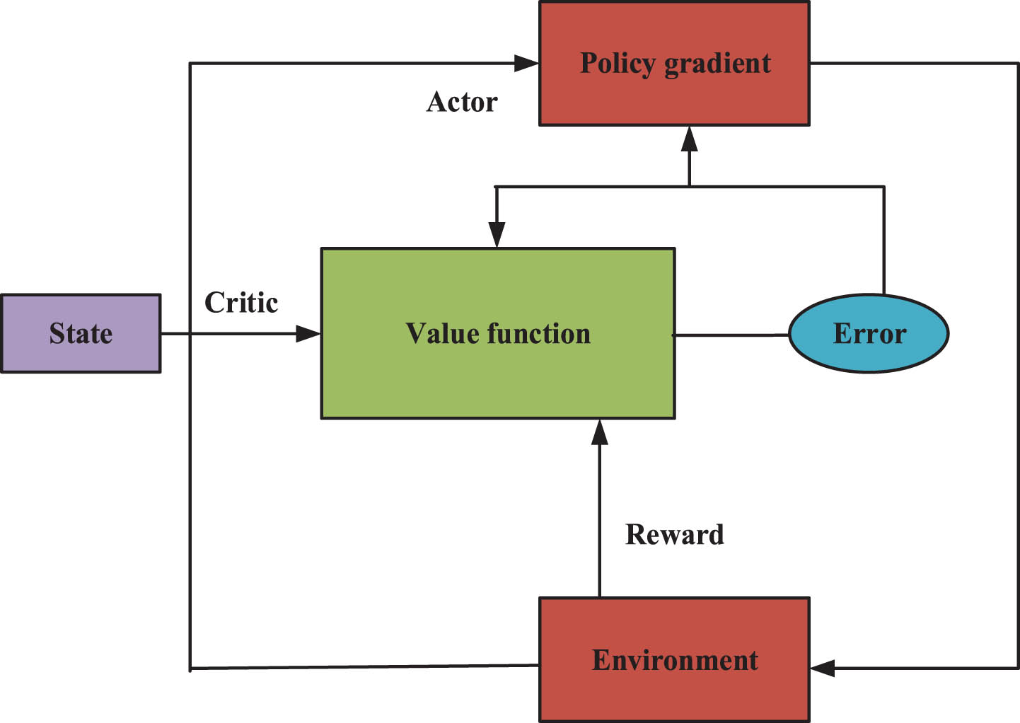
Architecture of the Actor-Critic algorithm.

The Critic is tasked with assessing the value of actions, with the overarching objective of learning a value function. The aim of a Critical network is to gauge the advantage of executing a specific action in comparison to the average level, thereby aiding the Actor in selecting the action more precisely. The Reward signifies the signal provided by the environment, contingent on the actions taken by the intelligent agent, and serves to evaluate the quality of these actions. This reward signal constitutes the pivotal feedback for the learning process of the intelligent agent.

The output of the Actor network is the probability distribution of various actions, representing the likelihood of taking different actions in the current state [23, 24]. The softmax function can be used at the output layer of the network to convert the original output into a probability distribution, ensuring that the sum of the probabilities of each output action is 1. This can explain the probability that the output of the network is in various categories, and it is convenient to understand and explain the prediction results of the network.

The formula for the softmax function is as follows. $P_{i} = \frac{e^{z_{i}}}{\sum_{j = 1}^{k} e^{z_{j}}}$ (7)

The output of Softmax function is continuous and changes smoothly with the change of the input, which is helpful to reduce the shock of gradient update and improve the stability of network training.

The training goal of the Actor network is to maximize long-term cumulative rewards by updating network parameters through the policy gradient method, so that the action probability can maximize the expected value of cumulative rewards.

A Critical network is typically comprised of several fully connected layers. Each layer employs a modified linear unit to facilitate nonlinear transformations, with the final layer delivering the value estimation of the state.

After establishing the Actor and Critic network, multiple agents can run simultaneously, allowing each agent to have its own Actor and Critic network. Intelligent agents independently interact with the environment in different environments and collect empirical data.

The architecture of the A3C algorithm is shown in Fig. 7. The intelligent agent asynchronously updates the global Actor and Critic networks. After collecting a certain amount of experience, each intelligent agent aggregates the experience data into a global memory and uses the data in the memory to update the global network parameters. The formula for updating strategy gradients is as follows.

Fig. 7

Architecture of the A3C algorithm.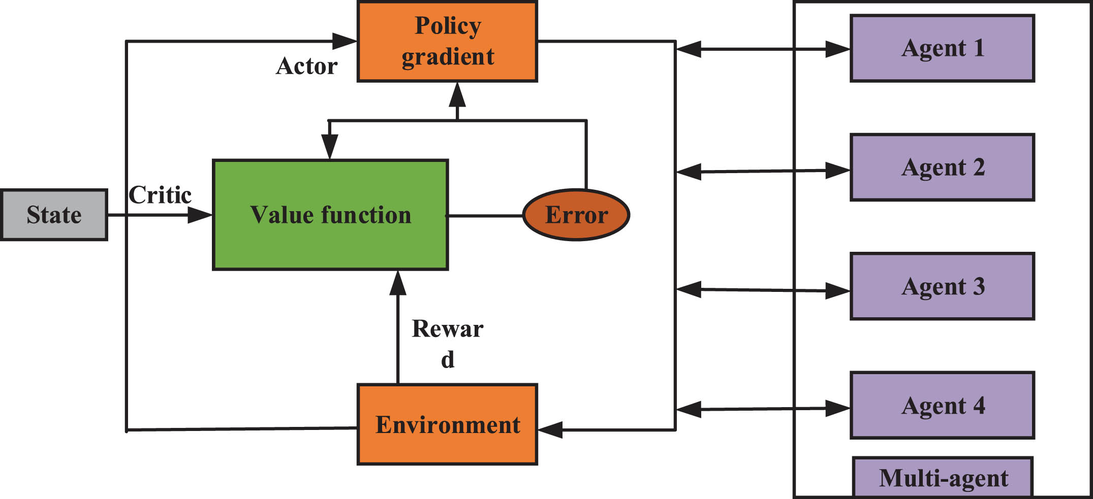

\nabla_{θ} J (θ) = E [\sum_{t = 0}^{T} \nabla_{θ} \log π_{θ} (α_{t} | s_{t}) A (s_{t}, α_{t})]

(8)

Where, ∇_θJ (θ) is the gradient of the objective function, π_θ (α_t|s_t) is the strategy of the Actor network, and A (s_t, α_t) is the dominant function.

The Critical network uses temporal differential error to update parameters and reduce the prediction error of state value. The formulas for updating the value function are as follows. $δ_{t} = r_{t} + γ V (s_{t + 1}) - V (s_{t})$ (9) $\nabla_{\emptyset} J (\emptyset) = \frac{1}{N} \sum_{t = 1}^{N} δ_{t} \nabla_{\emptyset} V (s_{t})$ (10)

Where, δ_t represents the temporal difference error, r_t represents the reward, γ represents the discount factor, and V (s_t) represents the value estimation of the critical network for the state.

Generally, the agents in this algorithm update asynchronously, with each agent independently collecting empirical data and using their own empirical data to update the global network parameters. This asynchronous update method can reduce the variance of updates and improve the stability and convergence speed.

The setting of reward function is the key to circuit structure optimization. The transforming of optimization objectives into reward signals can provide the learning direction and motivation for the intelligent agents. Therefore, with a reasonable reward function, intelligent agents can obtain the correct feedback signal based on the current circuit structure and design requirements, helping it better select actions and achieve its optimization.

The flow chart of the reward function is shown in Fig. 8.

Fig. 8

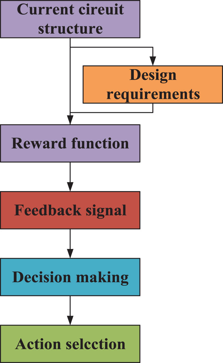
Flow chart of the reward function.

2.3 A3C model training

Adaptive optimization of the circuit structure can adeptly modify these structures to align with varying design specifications and environmental conditions, thereby catering to diverse application scenarios. Through the training of A3C model, intelligent agents possess the capability to autonomously learn and optimize circuit structures. The training process of A3C algorithm is shown in Fig. 9.

Fig. 9

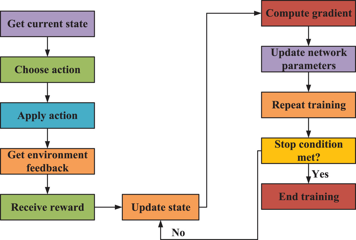
Training process of A3C algorithm.

The Actor network is responsible for learning strategies and selecting actions, while the Critic network is responsible for evaluating the value of states. In multiple parallel environments, the intelligent agents interact with the environment. These agents select actions from the Actor network based on the current state and apply them to the environment. The environment returns rewards and the next state based on the action and current state. It can calculate the gradients of the Actor and Critic networks, and update the parameters of the Actor and Critic networks with gradient descent methods. Asynchronous updates can be used, allowing each agent to independently update parameters in its own environment, thus achieving parallel training. However, A3C algorithm also has some limitations. A3C algorithm has the problems of long training time and large demand for computing resources, and its convergence speed is slow for complex problems. Therefore in circuit structure optimization, attention should be paid to the reasonable setting of convergence conditions and related parameters for the A3C model.

The update rule of gradient descent method is represented as follows. θ_new = θ_old - α ∇ _θJ (θ) (11)

Where, θ_old and θ_new represent the parameter values before and after the update, respectively. Gradient descent is a commonly used optimization method. By updating the parameters in the opposite direction of the loss function gradient, the network parameters can be adjusted to minimize the loss function. Asynchronous updating enables each agent to collect empirical data and update parameters independently, which speeds up the training process. In the paper, the parameters of Actor and Critic networks have been updated with gradient descent method to optimize the strategy and value function. The updating process of the gradient descent parameters is shown in Fig. 10.

Fig. 10

Updating process of the gradient descent parameters.

Fig. 11

Circuit structure of the switch audio power amplifier.

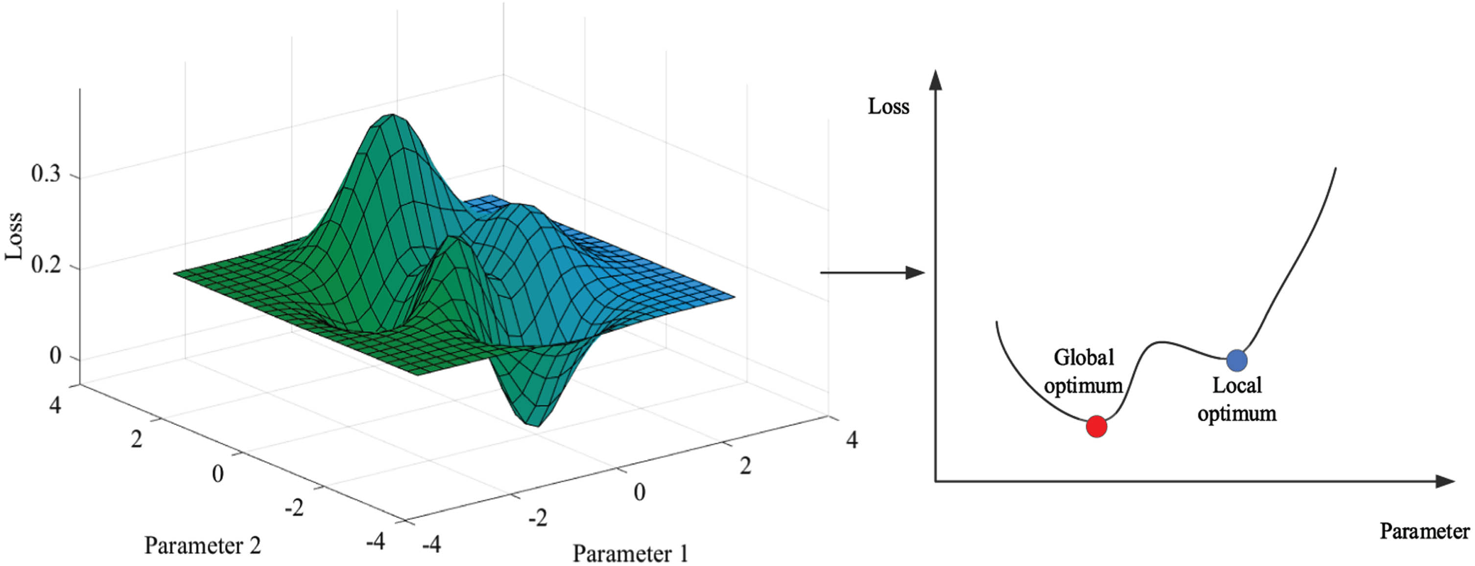
The gradient, defined as the rate of change in the loss function for each parameter, signifies the direction at which the loss function exhibits the most rapid alteration at a given parameter value. The computation for the gradient of the loss function on model parameters is facilitated through backpropagation. The gradient serves as a basis for updating the parameters. The gradient descent algorithm can strategically update the parameters along the direction of the loss function gradient, taking into account both its direction and magnitude. Consequently, this allows for a gradual approach to the minimum point of the loss function to converge towards the global optimal solution [25, 26].

3 Evaluation of adaptive optimization for the circuit structure

3.1 Simulation environment

The same electronic device may encounter a variety of application scenarios and operating conditions, including differing power supply voltages, operational temperatures, signal frequencies, etc. Traditional fixed structure circuits can’t often achieve optimal performance and power balance across these diverse scenarios [27, 28].

The adaptive optimization of circuit structure allows for the dynamic adjustment of circuit parameters in response to changing design requirements and actual working environments. This enables optimal performance under a variety of conditions [29, 30]. To assess the efficacy of this adaptive circuit structure optimization, in this paper, a dedicated circuit simulation environment has been constructed. The circuit structure of one switch audio power amplifier which is developed with A3C algorithm has been shown in Fig. 11. MATLAB has been used for the circuit simulation, which proves to be an effective and versatile method. When designing circuit structure for the switching audio power amplifier, it is crucial to consider both the characteristics of the amplifier and the design of the switching circuit. Within MATLAB, the Simulink tool can facilitate the establishment of this circuit structure. With its intuitive graphical interface, users can construct the circuit models, adjust parameters and conduct the simulation analysis [31].

The designed switching audio power amplifier has employed the 1 MHz switching frequency and used a feedback controller to ensure that the output voltage accurately tracks the 2 kHz and 2.5 kHz sine wave inputs. On/off state of the circuit is controlled with two N-Channel MOSFETs as switches.

The circuit structure of the Feedback controller, V_o, and Anti-alias filter has been shown in Fig. 12.

Fig. 12

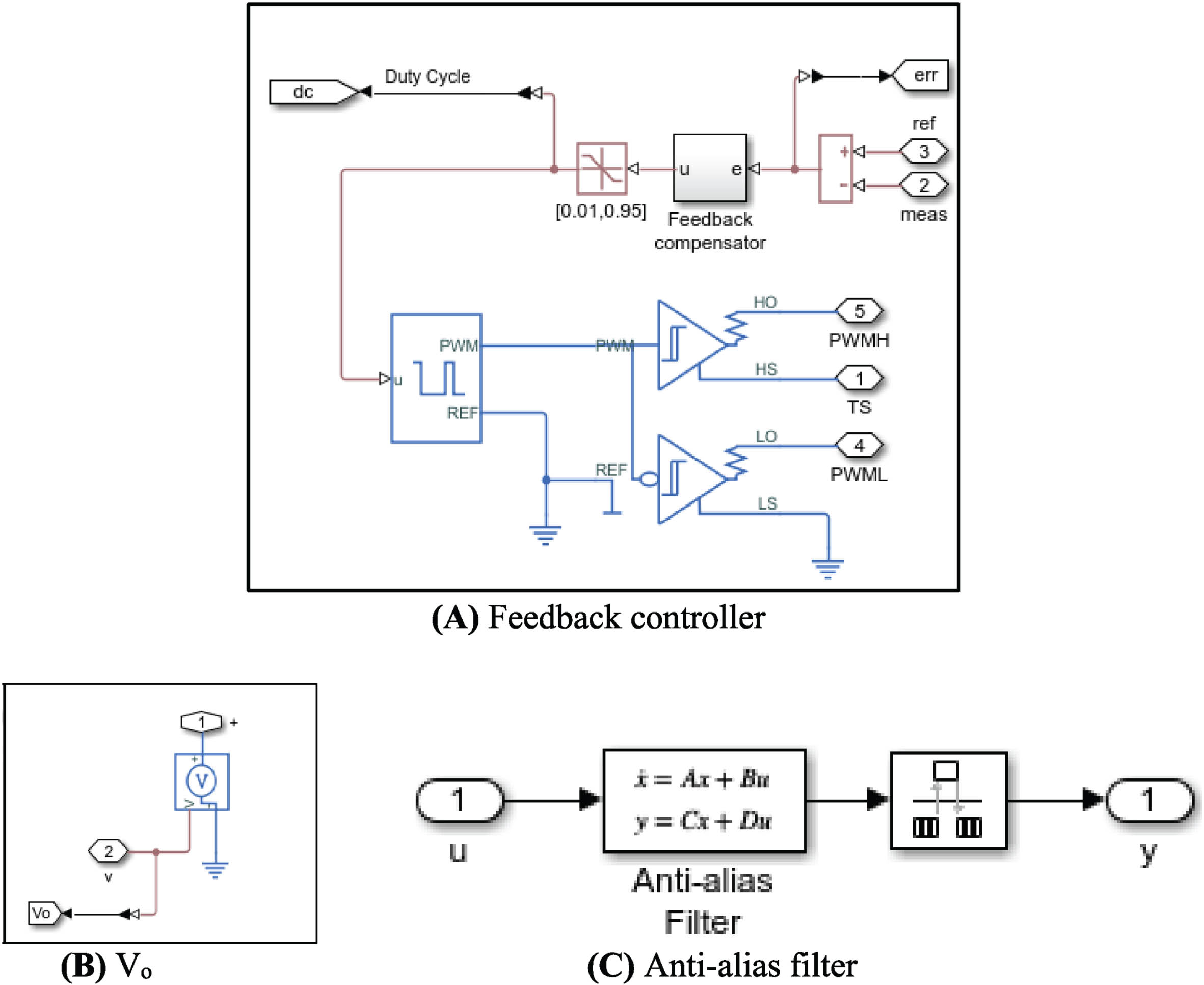
Structure of the feedback controller, Vo and Anti-alias filte.

In the study, the A3C model has been used for adaptive optimization of the circuit structure, constructing of which has used the TensorFlow module in Python. The learning rate is set at 0.001, with a batch size of 32, and the Adam optimizer has been utilized for the model optimization. To enhance the training efficacy of the A3C model, the NVIDIA GeForce RTX 4080 has been used to expedite the training process.

In the experiment, the A3C model has been designed to learn and adapt based on feedback from the environment. During the learning, the policy network can modifie the probability distribution of action selection, which can promote the model to take actions that enhance the circuit performance. As the model undergoes training, the rewards provided by the environment evolve in tandem with the optimization of the circuit structure. The model strives to maximize these rewards to optimize the circuit structure. The convergence speed can be assessed by examining the slopes of both the reward and loss curves. A quicker convergence speed indicates a stronger learning capability of the model, leading to superior optimization results.

3.2 Optimization evaluation

In this study, Adaptive Advantage Actor-Critic (A3C) has been employed for the adaptive circuit structure optimization. To effectively assess the impact of circuit structure optimization, a comparative analysis is conducted between A3C and other methodologies such as Actor-Critic, GA, and PSO. Using the known circuit structure, the simulation experiment has been carried out, and the optimization effect of the circuit structure with A3C model has been verified by the set indicators.

In the experiment, four primary parameters have been recognized as influence factors for the circuit structure optimization, which are gain, bandwidth, delay, and power consumption. In this paper, The circuit structure has been simulated, modeled and optimized for each iteration. Throughout this process, performance metrics such as gain, bandwidth, delay, and power consumption have been meticulously recorded and subsequently saved as evaluation outcomes. The efficacy of optimization can be discerned by scrutinizing these evaluation indicators.

4 Results and analysis

4.1 Results of gain optimization

The objective of gain optimization is to augment the signal gain of a circuit, thereby facilitating its capacity to amplify the input signal more effectively and deliver the requisite signal strength. This enhancement in gain allows for an increase in the amplitude of the signal, subsequently improving both the performance and efficiency of the circuit. The results derived from gain optimization employing four distinct algorithms have been shown in Fig. 13.

Fig. 13

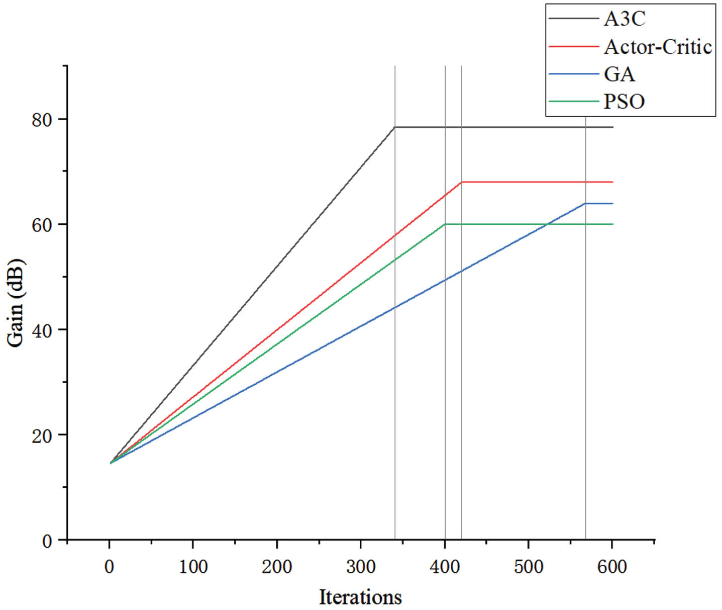
Results of gain optimization.

The horizontal axis denotes the number of algorithmic iterations, with a cumulative total of 600 recorded iteration data points. The vertical axis represents gain of the circuit structure of optimizations with four distinct algorithms. It is evident that, under the influence of these four algorithms, there is a consistent upward trend in circuit gain, eventually reaching a state of stability. The initial gain for A3C, Actor-Critic, GA, and PSO stands at 14.6 dB. The convergence gains for A3C, Actor-Critic, GA, and PSO are 78.4 dB, 68 dB, 64 dB, and 60 dB respectively. The gain of circuit structure optimizated with A3C surpasses that of Actor-Critic, GA, and PSO. This superiority can be attributed primarily to the adoption of a distributed strategy learning approach in A3C algorithm. By training multiple agents to investigate various facets of the circuit structure, A3C algorithm can exhaustively search the optimization space, identify superior circuit structures and consequently achieve greater gains. Besides, the convergence times for A3C, Actor-Critic, GA, and PSO are 340, 420, 568, and 400 respectively. A3C algorithm demonstrates its capability to effectively reduce the convergence time and markedly enhance the gain.

4.2 Results of bandwidth optimization

Optimizing the bandwidth of a circuit can reduce signal distortion and attenuation during transmission, thereby improving signal quality and accuracy. The results of bandwidth optimization using different algorithms have been shown in Fig. 14.

Fig. 14

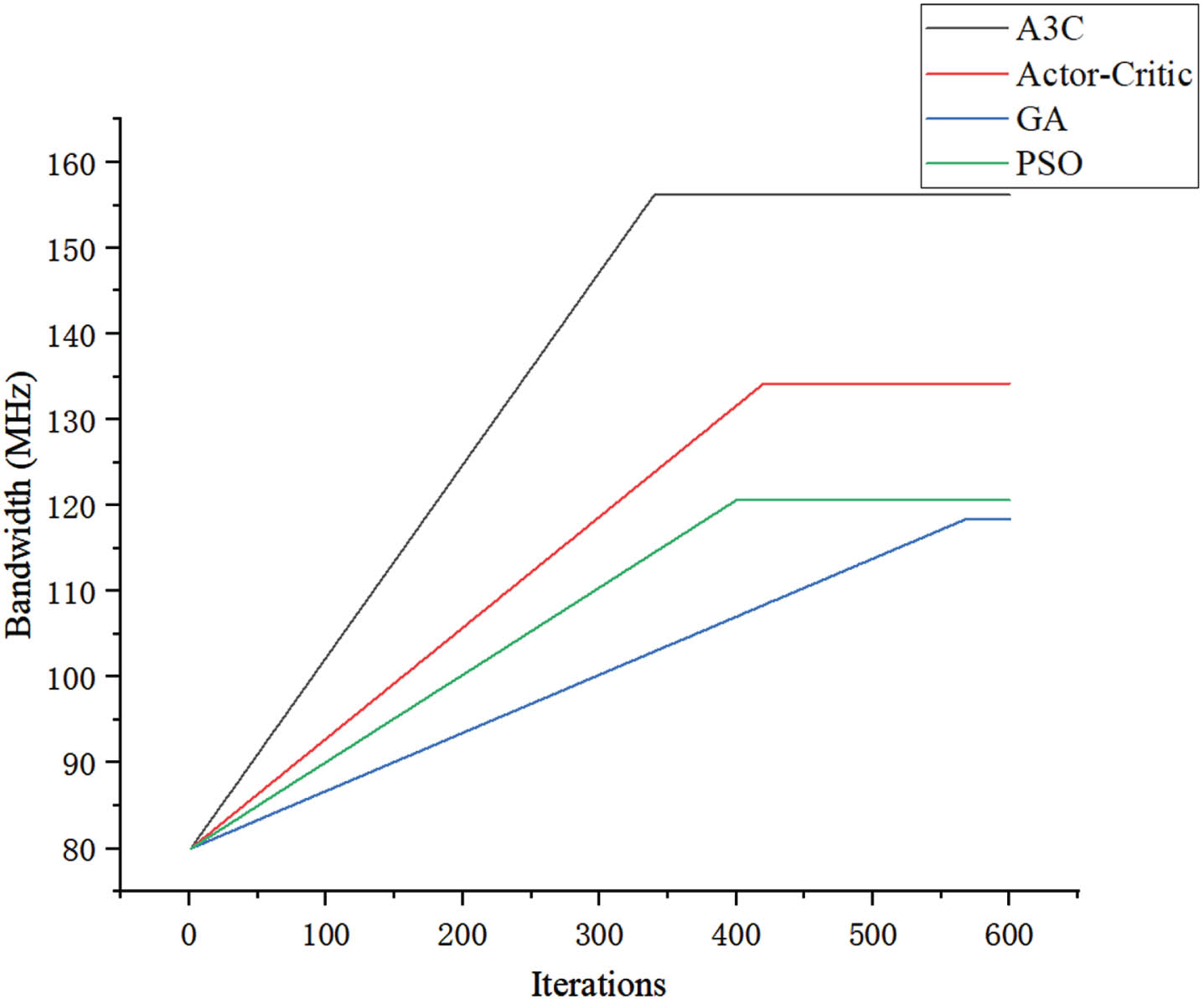
Bandwidth optimization results.

Among the four algorithms used for the optimization, A3C exhibits the most pronounced impact on bandwidth optimization. Initially, the circuit’s bandwidth has been set at 80 MHz. After the optimization, the bandwidth of A3C, Actor-Critic, GA, and PSO algorithms converge to 156.2 MHz, 134.2 MHz, 118.4 MHz, and 120.6 MHz respectively. In A3C algorithm, training multiple agents concurrently through parallelization and distributed learning make it capable for a more exhaustive exploration of the optimization space. In contrast, conventional optimization algorithms such as genetic algorithms and particle swarm optimization are susceptible to local optima.

4.3 Results of delay optimization

Optimizing circuit delay can enhance performance and response speed. The results of delay optimization using different algorithms have been shown in Fig. 15.

Fig. 15

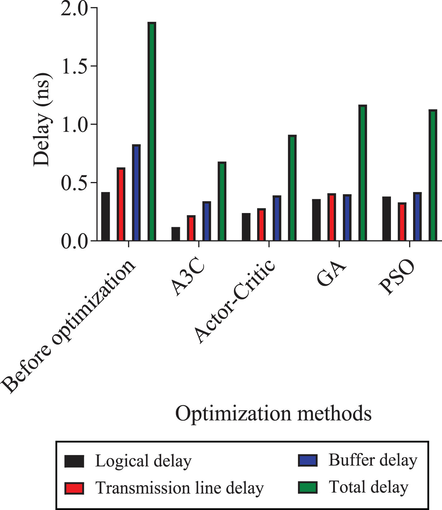
Delay optimization results.

The delays under consideration include logic delay, transmission line delay, and buffer delay, with the total delay being the cumulative sum of these three categories. The results indicate that irrespective of the specific algorithm employed for delay optimization, there is a significant reduction in delay data when compared to the delay preceding optimization. The A3C algorithm registers a logic delay of 0.12 ns, a transmission line delay of 0.22 ns, a buffer delay of 0.34 ns, and a total delay of 0.68 ns, which are all the lowest values among the four algorithms. It can be seen that the A3C algorithm has superior robustness and adaptability to initial conditions and environmental variations, attributed to its implementation of parallel training and diversity strategies.

In contrast, Actor-Critic algorithms may be more susceptible to the influence of initial conditions and environmental changes, leading to unstable optimization results.

4.4 Results of power consumption optimization

Excessive power consumption within circuits may lead to equipment overheating, compromising its performance and stability, and potentially causing damage to the electronic components. The results of power optimization using different algorithms have been shown in Fig. 16.

Fig. 16

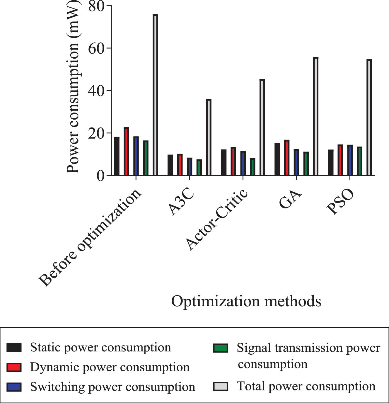
Power consumption optimization results.

The total power consumption encompasses static, dynamic, circuit switching, and signal transmission power. By optimizing power consumption, circuit energy and overall power usage can be reduced, which can also reduce strain on components and extend the service life of the entire circuit. When compared to the initial power consumption, optimizations with all the four algorithms have obtained a notable reduction in power consumption. The total power consumption for optimizations with A3C, Actor-Critic, GA, and PSO are 36 mW, 45.4 mW, 55.8 mW, and 54.9 mW respectively. Among the metrics of static, dynamic, circuit switching and signal transmission power consumption, optimization with A3C algorithm exhibits the best performance. All of this is attributed to that A3C algorithm excels in expediting the training process by integrating the training of multiple agents in parallel.

The comparison of the circuit optimization among the four algorithms include gain, bandwidth, delay and power consumption, which are all shown in Table 3. It can be seen the optimization objective function values for A3C, Actor-Critic, GA, and PSO algorithms respectively. Clearly, A3C algorithm is the best choice for the circuit structure optimization, and its optimization objective function value can reach 49.5, followed by Actor-Critic algorithm with the value of 39.0. In contrast, the optimization effects of GA and PSO are slightly inferior, being 31.4 and 31.1 respectively. The comparison emphasizes the remarkable effect of A3C in adaptive circuit structure optimization.

Table 3

Comparison of the optimization results

Index	A3C	Actor-Critic	GA	PSO
Gain (dB)	78.4	68	64	60
Bandwidth (MHz)	156.2	134.2	118.4	120.6
Total delay (ns)	0.68	0.91	1.17	1.13
Total power consumption (mW)	36	45.4	55.8	54.9
Optimization objective function value	49.5	39.0	31.4	31.1

5 Conclusions

In this paper, the A3C algorithm has been used to optimize the circuit structure, which can meet the complex and changeable design requirements. The basic principles of the A3C algorithm and the establishment and training process of the A3C model have been introduced in detail. Then a simulated circuit of the switching audio power amplifier has been used as the optimization object, and four algorithms including A3C algorithm have been applied for the experiment of the circuit structure optimization of the amplifier. All the experimental results demonstrates that the application of the A3C algorithm can effectively enhance gain and bandwidth while significantly reducing circuit delay and power consumption of the circuit, which is the algorithm with the best circuit optimization effect among the four algorithms used in this paper. However, the optimized circuit is not yet complex enough, and subsequent research will be conducted on the optimization effect of more complex circuits with the A3C algorithm.

Funding

The research work in this paper have been supported by Research and Exploration of Engineering Education Professional Accreditation System—Taking Bozhou College Electronic Information Engineering as an Example [grant number 2020jyxm1238], Research Center for Technology in Development of Embedded Systems [grant number GCBY202001], New Specialty Quality Improvement Project of Electronic Information Engineering [grant number 2022xjzlts027] and Cooperative Practice Education Base of Bozhou College Anhui Zhongke Zhibo Science and Technology Development Co., Ltd. [grant number 2023XJXM003].

Copyright

Authors submitting a manuscript do so in the understanding that they have read and agreed to the terms of the IOS Press Author Copyright Agreement posted in the ‘Authors Corner’ on www.iospress.nl.

References

Gao Lijiang , Yang Haigang , Li Wei , Hao Yanan , Liu Changlong , Shi Caixia , et al., An improved lookup table circuit structure and optimization method with the characteristics of high resource utilization, Journal of Electronics and Informatics 41 (2019), 2382–2388.

Meng Jinling , Zhao Hongda , Research on the structural design of circuit board tooling and its vibration transmission characteristics, Spacecraft Environmental Engineering 39(5) (2022), 489–495.

Sun Yu , Cao Lei , Chen Xiliang , Xu Zhixiong , Lai Jun , Review of research on in-depth reinforcement learning of multi-agents, Computer Engineering and Applications 56(5) (2020), 13–24.

Sun Changyin , Mu Chaoxu , Several key scientific issues of deep reinforcement learning of multi-agents, Journal of Automation 46(7) (2020), 1301–1312.

Guyue Huang , Jingbo Hu , Yifan He , Jialong Liu , Mingyuan Ma , Machine learning for electronic design automation: A survey, ACM Transactions on Design Automation of Electronic Systems (TODAES) 26(5) (2021), 1–46, DOI: https://doi.org/10.1145/3451179

Wei Ma , Zhaocheng Liu , Zhaxylyk Kudyshev

, Alexandra Boltasseva , Wenshan Cai , Yongmin Liu , et al., Deep learning for the design of photonic structures, Nature Photonics 15(2) (2021), 77–90.

Wang Xiaoqiang , Li Bin , Deng Chuanjin , Luo Jun , Yu Yongtao , Optimized design of vibration fixtures for complex integrated circuits packaged in CQFP for aerospace, Spacecraft Environmental Engineering 38(6) (2021), 662–669.

Feng Shanliang , Yang Bing , Chen Liang ,A timing optimization method for digital circuits based on time stealing, Microelectronics and Computers 40(8) (2023), 114–124.

Xiang Lin , Zhihui Jin , Fei Wang , Jian Luo , A novel bridgeless Cuk PFC converter with further reduced conduction losses and simple circuit structure, IEEE Transactions on Industrial Electronics 68(11) (2020), 10699–10708, DOI:10.1109/TIE.2020.3031527.

10.

Yi-Fei Pu , Bo Yu , Xiao Yuan ,Ladder scaling fracmemristor: A second emerging circuit structure of fractional-order memristor, Test 38(3) (2020), 104–111.

11.

Li Xin , Li Haiming , Ma Jian , An integrated model based on circuit structure analysis detects hardware trojan horses, Microelectronics and Computers 38(5) (2021), 80–86.

12.

Zhi Yuxin , Cai Xiaowu , Zhao Haitao , Xia Ruirui , Liu Hainan , Luo Jiajun , et al., A high-side drive circuit based on floating structure, Microelectronics and Computers 38(1) (2021), 7–11.

13.

Gholamreza Nikandish , Robert Bogdan Staszewski , Anding Zhu , Breaking the bandwidth limit: A review of broadband Doherty power amplifier design for 5G, IEEE Microwave Magazine 21(4) (2020), 57–75.

14.

Longjie Zhong , Jun Yang , Donglai Xu , Xinquan Lai , Bandwidth-enhanced oversampling successive approximation readout technique for low-noise power-efficient MEMS capacitive accelerometer, IEEE Journal of Solid-State Circuits 55(9) (2020), 2529–2538, DOI :10.1109/JSSC.2020.3005811.

15.

Jinquan Xu , Yutao Du , Boyi Zhang , Hao Fang , Hong Guo , Ye-Hwa Chen , et al., Sensorless fault-tolerant control with phase delay compensation for aerospace FTPMSM drives with phase open-circuit and short-circuit faults, IEEE Transactions on Industrial Electronics 68(6) (2020), 4576–4585, DOI :10.1109/TIE.2020.2988231.

16.

Bangxin Jiang , Jianquan Lu , Yang Liu , Exponential stability of delayed systems with average-delay impulses, SIAM Journal on Control and Optimization 58(6) (2020), 3763–3784, DOI: https://doi.org/10.1137/20M1317037

17.

Guo Chuncheng , Hao Xudan , Chen Fei , A new type of low-power SRAM read-write auxiliary circuit design, Journal of Beijing University of Aeronautics and Astronautics 46(8) (2020), 1618–1624.

18.

Wang Jiani , Zhou Zekun , Li Song , Shi Yue , Wang Zhuo , et al., A low-power and high-steady-state level displacement circuit, Microelectronics 50(3) (2020), 315–320.

19.

Atriya Biswas , Pier Giuseppe Anselma , Ali Emadi ,Real-time optimal energy management of multimode hybrid electric powertrain with online trainable asynchronous advantage actor–critic algorithm, IEEE Transactions on Transportation Electrification 8(2) (2021), 2676–2694, DOI:10.1109/TTE.2021.3138330.

20.

Alfonso Labao

, Mygel Andrei Martija

and Prospero Naval

, A3C-GS: Adaptive moment gradient sharing with locks for asynchronous actor–critic agents, IEEE Transactions on Neural Networks and Learning Systems 32(3) (2020), 1162–1176, DOI:10.1109/TNNLS.2020.2980743.

21.

Shuang Qiu , Zhuoran Yang , Jieping Ye , ZhaoranWang , On finite-time convergence of actor-critic algorithm, IEEE Journal on Selected Areas in Information Theory 2(2) (2021), 652–664, DOI:10.1109/JSAIT.2021.3078754.

22.

Andrew Barto

, Richard Sutton

and Charles

, Looking back on the actor–critic architecture, IEEE Transactions on Systems, Man, and Cybernetics: Systems 51(1) (2020), 40–50. DOI: 10.1109/TSMC.2020.3041775.

23.

Oguzhan Dogru , Kirubakaran Velswamy , Biao Huang ,Oguzhan Dogru, Kirubakaran Velswamy and Biao Huang, Actor–critic reinforcement learning and application in developing computer-vision-based interface tracking, Engineering 7(9) (2021), 1248–1261, DOI: https://doi.org/10.1016/j.eng.2021.04.027

24.

Yanwei Jia , Xun Yu Zhou ,actor-critic learning in continuous time and space: Theory and algorithms, The Journal of Machine Learning Research 23(1) (2022), 12603–12652.

25.

Shi Jiarong , Wang Dan , Shang Fanhua , Zhang Heyu ,Research progress on stochastic gradient descent algorithm, Journal of Automation 47(9) (2021), 2103–2119.

26.

Mi Yang , Peng Jianwei , Chen Boyang , Wang Xiaomin , Liu Zixu , Wang Yufei , et al., The microgrid is completely distributed and optimized scheduling based on the consistency principle and gradient descent method, Power System Protection and Control 50(15) (2022), 1–11.

27.

Xu Jianqing , Gao Yong , Yang Yuan , Meng Zhaoliang , Wen Yang , Zhang Le , et al. SiC MOSFET drive circuit design and characteristic analysis, Semiconductor Technology 45(5) (2020), 352–358.

28.

Ma Sheng , Shen Li , Wang Yongjun , Tang Yuhua , Tang Zhensen , Wang Zhiying , et al., Exploration on the construction of a practical teaching system for the training of integrated circuit design talents in the context of new engineering,, Laboratory Research and Exploration 41(1) (2022), 206–210.

29.

Zulqurnain Sabir , Muhammad Asif Zahoor Raja , Sharifah

, Alhazmi , Applications of artificial neural network to solve the nonlinear COVID-19 mathematical model based on the dynamics of SIQ, Journal of Taibah University for Science 16(1) (2022), 874–884.

30.

Adnène Arbi ,, Controllability of delayed discret fornasini-marchesini model via quantization and random packet dropouts, Mathematical Modelling of Natural Phenomena 17 (2022), 38.

31.

Bellili , Nour El Imane , Khaled Bekhouche , Class-D Audio Amplifier using Sigma-Delta (ΣΔ) Modulator, Indonesian Journal of Electrical Engineering and Informatics (IJEEI) 10(3) (2022), 567–572.